國 立 交 通 大 學
電子工程學系 電子研究所碩士班
碩 士 論 文
用於影像壓縮之方向性多重解析度轉換
和區塊位元平面算數編碼
Directional Multiresolution Transform
And
Block-based Bitplane Arithmetic Coding
For Image Compression
研究生: 徐漢光
指導教授: 杭學鳴 博士
用於影像壓縮之方向性多重解析度轉換
和區塊位元平面算數編碼
Directional Multiresolution Transform and
Block-Wise Bitplane Arithmetic Coding for Image
Compression
研 究 生:徐漢光
指導教授:杭學鳴 博士
S t u d e n t : H a n - K u a n g S h u
Advisor: Dr. Hsueh-Ming Hang
國 立 交 通 大 學
電子工程學系 電子研究所碩士班
碩
士
論
文
A Thesis
Submitted to the Institute of Electronics
College of Electrical Engineering and Computer Science National Chiao Tung University
in Partial Fulfillment of Requirements for the Degree of
Master of Science in
Electronics Engineering June 2005
Hsinchu, Taiwan, Republic of China
授權書
(博碩士論文) 本授權書所授權之論文為本人在_______大學(學院)______系所 ______組_____學年度第___學期取得___士學位之論文。 論文名稱:_____________________________ 1.□同意 □不同意 本人具有著作財產權之論文全文資料,授予行政院國家科學委員會科學技術資 料中心、國家圖書館及本人畢業學校圖書館,得不限地域、時間與次數以微縮、 光碟或數位化等各種方式重製後散布發行或上載網路。 本論文為本人向經濟部智慧財產局申請專利的附件之一,請將全文資料延後兩 年後再公開。(請註明文號: ) 2.□同意 □不同意 上述授權內容均無須訂立讓與及授權契約書。依本授權之發行權為非專屬性發 行權利。依本授權所為之收錄、重製、發行及學術研發利用均為無償。上述同 意與不同意之欄位若未鉤選,本人同意視同授權。 指導教授姓名: 研究生簽名: 學號: (親筆正楷) (務必填寫) 日期:民國 年 月 日 1. 本授權書請以黑筆撰寫並影印裝訂於書名頁之次頁。 2. 授權第一項者,所繳的論文本將由註冊組彙總寄交國科會科學技術資料中 心。 3. 本授權書已於民國 85 年 4 月 10 日送請內政部著作權委員會(現為經濟部智 慧財產局)修正定稿。 4. 本案依據教育部國家圖書館 85.4.19 台(85)圖編字第 712 號函辦理。國立交通大學
論文口試委員會審定書
本校___________________碩士班___________________君 所提論文_________________________________________ 合於碩士資格水準,業經本委員會評審認可。 口 試 委 員 : _________________ _________________ _________________ 指 導 教 授 : _________________ 所 長 : _________________ 系 主 任 : _________________ 中華民國九十四年 月 日用於影像壓縮之方向性多重解析度轉換
和區塊位元平面算數編碼
研究生:徐漢光
指導教授:杭學鳴
國立交通大學 電子工程學系 電子研究所碩士班
摘要
連續畫面小波視訊轉換(Interframe Wavelet Video Coding)擁有訊雜比可調 性、時間軸上可調性和畫面解析度可調性的好處,小波轉換在此編碼架構中扮演 重要角色,另外算數編碼器在整體編碼中也是一個不可忽略的要件,因為算數編 碼器產生影像壓縮的最後位元串流。 我們實驗平台的來源是MPEG 可調式影像編碼核心實驗參考軟體,藉著修 改參考軟體架構來實現本論文的想法。 在本論文共包含兩個研究主題,其中一個主題針對是加化熵編碼效率的方 法,並在實驗中將這方法整合到連續畫面小波視訊轉換的架構中。主要原理是根 據能量聚集來提昇編碼效率,實驗的結果可以看到編碼位元數量的減少,然而要 使這方法有更高效率是需要更深入的研究。 另外一個研究是將原本連續畫面小波視訊轉換架構的空間轉換替代成方向 性多重解析轉換。方向性多重解析轉換主要是以Minh N. Do 提出的階層式方向 性濾波組為基礎,將圖片分解成不同解析度和方向性的成分。在最後的模擬結果 可以看到在高壓縮比率下訊雜比和視覺品質會較原方法提升。
Motion Information Scalability for
Interframe Wavelet Video Coding
Student: Han-Kuang Shu Advisor: Dr. Hsueh-Ming Hang
Department of Electronics Engineering & Institute of Electronics
National Chiao Tung University
Abstract
Interframe wavelet coding has the advantage of SNR, temporal, and spatial scalability. Wavelet Transform Coding is one of the most essential components in the interframe wavelet coding architecture. The arithmetic entropy subsystem is another indispensable element in Wavelet Transform Coding. It produces the final compressed output bit stream.
This thesis contains two major topics. One is an enhanced entropy coding scheme that can be incorporated into the interframe wavelet coding architecture. Another topic is replacing the original separable wavelet by the directional multiresolution transform.
We modify the entropy coding syntax/scheme originally used in the MPEG SVC Core Experiment (CE) reference software. We take the advantage of energy clustering properly to improve coding efficiency. We have observed some bit savings of this technique in our simulations under the conditions specified by the MPEG core
experiments; however, the full potential of this technique is yet to be further explored. The directional multiresolution transform decomposes an image into different resolution and direction components. It seems to be a more compact and efficient representation of images. We use the directional filter back to replace the separable wavelet in the MPEG wavelet software. The improvement of PSNR and visual quality can be observed on the low bitrate compressed images.
誌 謝
首先感謝家人在我的背後默默的支持,讓我能夠專注在自己的研究上,也謝 謝杭學鳴老師細心指導,並在面臨瓶頸時拉我一把。
最後感謝實驗室的伙伴們,祥哲學長、家揚學長、崑健學長、朝雄、志楹、 盈閔、思浩、承毅、世騫、景中……,你們讓我的研究生生活變的多彩多姿。
Content
Chapter 1...1
Chapter 2...3
2.1 Video Coding Methods ...3
2.2 Subband Coding...7
2.2.1 Temporal Decomposition...9
2.2.2 Spatial Decomposition ...10
Chapter 3...13
3.1 What is Scalable Coding? ...13
3.2 MPEG SVC Reference Software ...14
3.3 Disadvantage of Wavelet-Based Coder...14
3.4 Temporal Decomposition of Interframe Wavelet...15
3.5 Spatial Decomposition ...16
3.6 Entropy Coding — 3D EBCOT...17
3.6.1 Codeblock Partition ...17
3.6.2 Zero coding, Sign coding and Magnitude Refinement ...19
3.6.3 Significant Propagation Pass, Magnitude Refinement Pass and Normalization Pass ...24
3.7 SNR/Rate, Spatial and Temporal Scalability ...25
3.7.1 SNR/Rate Scalability ...25
3.7.2 Spatial Scalability ...26
3.7.3 Temporal Scalability ...27
Chapter 4...28
4.1 Introduction...28
4.2 Proposed Entropy Coding Scheme ...29
4.2.1 SB-Reach Method...29
4.2.2 Syntax and Architecture Change...32
4.3 Coding Procedure...33
4.3.1 Definition ...33
4.3.2 Coding steps...34
4.4 Simulation Results ...35
4.5 Appendix A: PSNR value...37
4.6 Appendix B: Statistics of SB-Reach Depth and Block Size ...40
Chapter 5...43
5.1. Motivation...43
5.2 Contourlet ...44
5.4 Directional Filter Bank ...48
5.4.1 Fan Filter Design...50
5.4.2 Quincunx Sampling Lattice ...55
5.4.3 Patterns of Sampled Images...55
5.4.4 Equivalent Representation of DFB ...58
5.4.5 The Architecture of Directional Filter Bank ...62
5.5 Pyramidal Directional Filter Bank ...64
5.6 Experiments and Results...65
Chapter 6...75
List of Tables
Table 3.1: Spatial analysis filter...17
Table 3.2: Context assignmetn map of zero coding...22
Table 3.3: Context assignment map of sign coding ...23
Table 4.1: Bitrate savings (in percentage) for the FOREMAN and BUS sequences of the H frames at temporal levels 1 and 2. ...36
Table 4.2: Bitrate savings (in percentage) of the H frames at temporal levels 3 and 4. ...36
Table 4.3: Bitrate savings (in percentage) at the bottommost temporal level. ...37 Table 4.4 : PSNR of CREW...37 Table 4.5: PSNR of HARBOUR...38 Table 4.6: PSNR of SOCCER...38 Table 4.7: PSNR of CITY...38 Table 4.8:PSNR of BUS...39 Table 4.9: PSNR of FOOTBALL ...39 Table 4.10: PSNR of FOREMAN...39 Table 4.11: PSNR of MOBILE ...40
Table 4.12: Bit saving ratio and overhead ratio for BUS, FOOTBALL and FOREMAN ...42
Table 5.1: 9/7 filter taps ...47
Table 5.2: The base coefficients of 23-45 fan filters...50
Table 5.3: PSNR of Barbara...67
Table 5.4: PSNR of fingerprint ...68
Table 5.5: The PSNR list of Lena ...68
List of Figures
Figure 2.1: Classification of video CODEC (MCP: motion compensated prediction, TSB: temporal subband decomposition, MCTF: motion
compensated temporal filtering)...4
Figure 2.2: The signal-based coding structure...5
Figure 2.3: The motion vector prediction on two temporal neighboring frames and motion vector information is generated...6
Figure 2.4: With a reference frame and motion information, original frame could be generated...6
Figure 2.5: Typical 3-D subband decomposition. The numbers on leaves of the tree structure (a) correspond to subband partitions on (b)...8
Figure 2.6: Temporal decomposition. Left: low-pass filtering. Right: high-pass filtering...9
Figure 2.7: Temporal filtering with motion compensation. Left: low-pass frame. Right: high-pass frame...10
Figure 2.8: An example of “Lena” after transform ...10
Figure 2.9: Octave-based frequency partition... 11
Figure 2.10: Another frequency decomposition arrangement...12
Figure 3.1: The block diagram of 3D subband video coding...14
Figure 3.2: An example of temporal decomposition on GOP = 16...15
Figure 3.3: Spatial decomposition of a picture ...16
Figure 3.4: The codeblock assignment about a subband smaller than defined codeblock size - 64x64...18
Figure 3.5: The codeblock assignment when a subband is larger than defined codeblock size - 64x64...19
Figure 3.6: An example of bit-plane decomposition and coding method. The scanning order is from most significant bitplane to less significant bitplane. ...20
Figure 3.7: The neighbor of the coefficient considered into context model.21 Figure 3.8: the arrangement of encoded bit stream...25
Figure 3.9: SNR/rate scalability can be achieved by truncating the embedded bit-stream. The PSNR performance is increased when bit-rate increase...26
Figure 3.10: An example of resolution increasing by 2D wavelet transform ...27
mapping block bits ...30 Figure 4.2: Examples of square mapping block of n by n coefficients on a
bitplane ...30 Figure 4.3: Construct the SB-reach planes up to the selected “SB-reach
plane.” ...31 Figure 4.4: The encoding process of the SB-reach plane and its associated
coefficient bit-plane...32 Figure 4.5: Changes between the original and the proposed syntax...33 Figure 4.6: (a) Block size distribution and (b) SB-reach depth distribution of BUS ...40 Figure 4.7: (a) Block size distribution and (b) SB-reach depth distribution of FOOTBALL ...41 Figure 4.8 (a) Block size distribution and (b) SB-reach depth distribution of
FOREMAN ...41 Figure 4.9: ‘a’ the original bitstream without SB-reach method and the
bitstream ‘b+c’ is the one with SB-reach method. ‘b’ means the overhead of SB-reach method and ‘c’ means the reduced size bitstream ‘a’ after using SB-reach method. ...42 Figure 5.1: Block diagram of Pyramidal directional filter bank. Multiscale
decomposition is at the first stage. Down sampling is applied on the lower frequency band and higher frequency band is followed by a directional filter bank. ...45 Figure 5.2: Illustration of the “ frequency scrambling.” Upper: spectrum
after high-pass filtering. Lower: spectrum after high-pass filtering and downsampling. We can see that the high-pass spectrum is folded back into the low frequency region...46 Figure 5.3: The analysis side of LP scheme. C is the coarse version of
original image and D is the difference between C and input X. ...47 Figure 5.4: The synthesis side of the LP scheme. X’ is the reconstructed
image. ...47 Figure 5.5: DFB with the level of tree structure n = 3 and there are 2 of 3
frequency partition regions. ...48 Figure 5.6: QFB with sub-lattice sampling Q and fan filters. This also forms
the first level of DFB with two directions...49 Figure 5.7: Quincunx sampling lattice...49 Figure 5.8: Ideal diamond-shaped filter...51 Figure 5.9: H0(z z ) designed with 6 base taps...52 0, 1
1
value 0 and 1on the axis represent -π and π. The value 0.5 means
frequency value 0...52
Figure 5.11: The modulated diamond-shaped filter - H0(z0,z1) form the fan filter. ...53
1 Figure 5.12: Illustration of DC level in DFB. The DC level of Y0 is half of Y1 because of the different DC levels of H0(z z ) and H1(0, 1 z z ) ...54 0, Figure 5.13: (a) The original image...55
Figure 5.14: Square-like discrete representation. ...56
Figure 5.15: (a) Data partition of a rectangular-shaped image. ...56
Figure 5.16: The pattern of a diamond-shape like image. ...57
Figure 5.17: (a) An example of the diamond-shaped image. (b) and (c) are sampled data from (a) under the critical sampling condition. When (b) and (c) are combined to reconstruct (a), (c) have to be shifted to avoid in case of data overlapping. ...58
Figure 5.18: Block diagram of QFB with resampling operation ...59
Figure 5.19: An example of the resampling operation- R0. Note that the data coordinates are changed by the “upsampling” process, although the data rate does not increase nor decrease. ...59
Figure 5.20:Resampled images in four cases...60
Figure 5.21: An example of the third level in DFB. Left: the original block diagram. Right: the equivalent block diagram. ...61
Figure 5.22: The image of downsampling by P0...61
Figure 5.23: The architecture of 4-directions filter bank. ...62
Figure 5.24: The architecture of 8-directions filter bank. The first and second stages are extended from the 4-directions filter bank. The additional sampling processes are on the third stage. ...63
Figure 5.25: The architecture of 8-directions filter bank. The equivalent diagram replace the original diagram (Figure 5.24) on the third level. ...64
Figure 5.26: The block diagram of PDFB. Multiscale decomposition is first applied to generate the low-pass and high-pass images. The low-pass image can be further decomposed using the same structure on the next level. A directional decomposition is applied to each high-pass channel...65
Figure 5.27: The block diagram of PDFB. In the experiments, low-pass channel generates the coarse resolution image. The high-pass image is passed to different directional decompositions at different levels. ...66 Figure 5.28: The corresponding frequency partition of architecture in Figure
Figure 5.29: PSNR performance comparison of MSSVC, JPEG2000 and MSSVC_MST for Barbara...67 Figure 5.30: PSNR performance comparison of MSSVC, JPEG2000 and
MSSVC_MST for fingerprint. ...68 Figure 5.31: PSNR performance comparisons of MSSVC, JPEG2000 and
MSSVC_MST for Lena...69 Figure 5.32: PSNR performance comparison of MSSVC, JPEG2000 and
MSSVC_MST for peppers. ...69 Figure 5.33: The reconstructed image of fingerprint at the compression ratio of 0.9375 (a) The reconstructed image by using MDT, (b) The reconstructed image by using original scheme-wavelet. ...72 Figure 5.34: Reconstructed image “barbara” at the compression ratio 1.25%. (a) MDT, (b) the original MSSVC scheme. ...74
Chapter 1
Introduction
Video applications have been playing an important role in our daily life in decades with improvement in digital technologies. The applications can be a low delay issue for interactive videophone systems, low bit rate requirements for mobile devices, and high quality high-definition television (HDTV) or DVD in our living room.
In resent years, H.264 is the most effective video compression standard in single layer coding. Beyond single layer coding, video stream with scalable ability has gain more and more attention recently for its flexibility in resolution, frame rate and quality. However, the performance of the scalable video coding still can’t compete with single layer coding especially on the low bit rate condition. In this thesis, we focus on the
The thesis contains two independent subjects. One is considering directional contents in spatial transform and replacing the original transform scheme-wavelet. Another is inducting block-wise arrangements in entropy coding module to utilize the
phenomenon of energy clustering on bitplanes. The experiments are based on the reference software of MPEG scalable video coding group proposed by Microsoft.
The thesis is organized as follows. In Chapter 2, the fundamentals of video coding. Chapter 3 briefly describes the schemes of each module in our reference software. The method and result of the block-wise bitplane arithmetic coding is presented in Chapter 4. The directional Multiresolution transform is illustrate and evaluated in Chapter 5.
Chapter 2
Video Coding
2.1 Video Coding Methods
Video applications have been playing an important role in our daily life in decades with improvement in digital technologies. The applications can be a low delay issue for interactive videophone systems, low bit rate requirements for mobile devices, and high quality high-definition television (HDTV) or DVD in our living room. In last twenty years, digital video compression advances very fast, and many techniques are developed. Based on their underlying technologies, these techniques can be classified into several classes as shown in Figure 2.1.
Figure 2.1: Classification of video CODEC (MCP: motion compensated prediction, TSB: temporal subband decomposition, MCTF: motion compensated temporal filtering)
Video CODEC can be firstly classified into model-based and signal-based. If the coding algorithms analyze objects on video frames and adjust coding parameters according to the analysis results, these coding algorithms are called “model-based video coding.” We call a algorithm “signal-based video coding”, if its coding process doesn’t contain an explicit model. A model-based coding algorithm needs to construct and model the object in a video sequence. Therefore, the requirement of computation is high and the complexity increases. For these reasons, the model-based coding algorithm often targets on the synthetic video. On the other hand, signal-based coding methods have a less complicated architecture because there are no object contents and the process treat the sequence as usual signal. The structure is shown in Figure 2.2.
Temporal decomposition (motion vector prediction,
motion vector search, MCTF...etc) Spatial decomposition (DCT, wavelet transform...etc) Quantization (quantization step...etc) Entropy coding (variable length coding,
CABAC, EZBC...etc)
Figure 2.2: The signal-based coding structure.
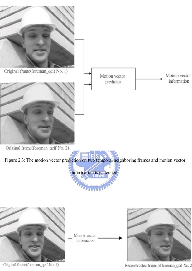
A video sequence can be divided into three dimensions: temporal, horizontal and vertical. We often decompose the video sequence by these dimensions. In temporal axis, the neighboring frames are highly correlated, and using motion vector prediction can reduce the inter-frame redundancy. Figure 2.3 shows the block diagram of motion compensated prediction (MCP) that generate motion information and Figure 2.4 shows an example of the frame reconstructed by a reference frame and motion information.
Figure 2.3: The motion vector prediction on two temporal neighboring frames and motion vector information is generated.
Figure 2.4: With a reference frame and motion information, original frame could be generated.
Unlike MCP using motion information to reduce temporal redundancy, temporal subband decomposition (TSB) treats temporal signal as usual signal and 3-D filtering
process is performed on video. If TSB coder were incorporated with motion compensation, we call it “TSB with MC.” The horizontal and vertical signal is processed by spatial analysis. DCT or wavelet transform is applied to translate signal into frequency domain. Generally speaking, lower frequency bandx often carry the most information within a frame. With this property, compression efficiency could be improved.
2.2 Subband Coding
As described in the previous section, a video sequence can be decomposed according to three axis - temporal, vertical and horizontal. Vertical and horizontal data are often inducted into spatial signal. Temporal and spatial signal have different properties in analyzing methods. If we analysis the temporal frequency of two neighboring frames from a sequence, the low frequency of temporal signal is
intuitionally the same part of two frames and the high frequency is the difference part. When a sequence contains large motions, the energy of temporal high frequency is larger than that of a sequence with small motions. DCT or wavelet transform is used most frequently in spatial analysis. After applying spatial transform, frequency
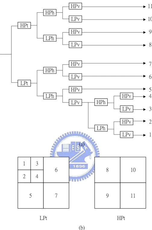
components of a frame can be classified from low frequency to high frequency. Figure 2.5 shows one kind of 3D-subband decomposition.
1 2 3 4 5 6 7 8 9 10 11 HPt HPh HPv LPv LPh HPv LPv HPh HPv LPv LPh HPv LPv LPt HPh HPv LPv LPh HPv LPv 11 10 9 8 7 6 5 4 3 2 1 LPt HPt (a) (b)
Figure 2.5: Typical 3-D subband decomposition. The numbers on leaves of the tree structure (a) correspond to subband partitions on (b).
HPt: The high frequency subband signal after temporal decomposition. LPt: The low frequency subband signal after temporal decomposition. HPh: The high frequency subband signal after spatial horizontal decomposition.
HPv: The high frequency subband signal after spatial vertical decomposition. LPv: The low frequency subband signal after spatial vertical decomposition.
2.2.1 Temporal Decomposition
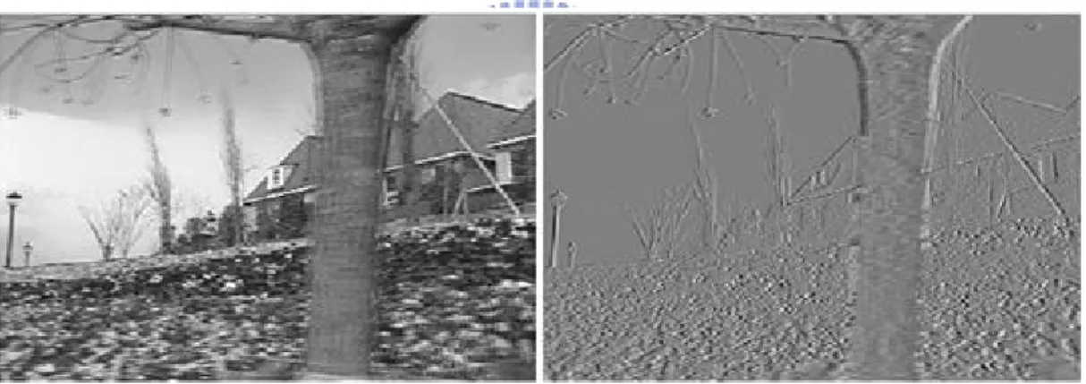
Traditionally, Haar filter is often used on temporal subband decomposition. With low-pass and high-pass filter applied on the same pixel position in temporal axis, low frequency signal is gathered on one frame and high frequency is on another frame as shown in Figure 2.6. We can observe that the energy of temporal high frequency frame is not reduced to zero and low frequency frame is blurred. It means the energy compaction of temporal subband filtering is not performed very well.
Figure 2.6: Temporal decomposition. Left: low-pass filtering. Right: high-pass filtering
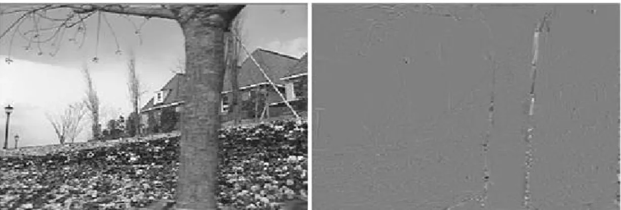
Kronander[1] proposed another filtering method cooperated with motion
estimation. At first, motion estimation is performed on two consecutive frames, then, the reconstruction frame is generated by first frame and backward motion vector. Using second frame and the reconstructed frame generate the temporal high-pass frame. Then, the high-pass frame and the first frame create the low-pass frame. The result is shown in Figure 2.7. Better energy compaction can be observed.
Figure 2.7: Temporal filtering with motion compensation. Left: low-pass frame. Right: high-pass frame
2.2.2 Spatial Decomposition
A frame can be separated into several subbands. These subbands have different frequency range in horizontal and vertical. With different analysis and synthesis filters, the properties of these subbands affect the performance of quantization and
rate-distortion. In video coding architecture, quantization and rate-distortion are connected next by spatial decomposition.
Wavelet transform is the most popular subband transform and well localized, unlike DCT, in both space and frequency. It removes spatial redundancy and have good energy compaction. Figure 2.8 is an example of the wavelet transform.
According to times that wavelet transform performed on each subband, there are many ways to decompose an image. An octave-based frequency partition, which is one kind of partition type and seen in EZW[3], SPITE[4] and EZBC[5][6], is shown in Figure 2.9.
Figure 2.9: Octave-based frequency partition (LL: low frequency band in horizontal and vertical, LH: low frequency in horizontal and high frequency in vertical HL: high frequency in horizontal and low frequency in vertical
HH: high frequency in both horizontal and vertical)
In MPEG SVC (scalable video coding) group, the spatial decomposition of the wavelet-based reference software is as shown in Figure 2.10.
Figure 2.10: Another frequency decomposition arrangement.
In this decomposing flow, based on octave-based frequency partition, the HL, LH and HH bands generated by first level wavelet decomposition are further performed DWT.
Shapiro[3], the pioneer in embedded coding scheme, proposed EZW in 1992. This work attracted a lot of research interests and many fallow-up works have been proposed such as SPITE , EZBC and EBCOT[7][8]. EBCOT (Embedded Block Coding with Optimized Truncation) is an efficient and remarkable embedded coding scheme proposed by Taubman. Unlike EZW or SPITE which introduces inter-band dependency, EBCOT only utilizes intra-band dependency. The coding techniques based on the concepts of EBCOT, such as sequential bit plane coding and effective R-D optimization, are adopted by the JPEG2000 international standard.
Chapter 3
Scalable Video Coding
3.1 What is Scalable Coding?
Generally speaking, scalable functionalities can be divided into spatial, temporal, SNR and bit rate. The purpose of scalability is that a minimal bit-stream can be extracted from a video bit-stream, already coded by a scalable video coder, for the least video requirements in resolution, frame rate and PSNR. When an application requests a better quality in either resolution or bit rate, we only to extract additional bit-stream that matches the request and add to the original bit-stream. Thus, this bit-stream organization is “embedded”. Video coders with scalability should produce the afore mentioned embedded bitstream, to allow video receiver decoding at different resolution, frame rate and quality.
3.2 MPEG SVC Reference Software
SVC received a lot of attention for its flexibility on applications. Therefore, the MPEG group started activity on this subject in 2004. According to the spatial
transforms used, the proposed standard candidates can be basically classified into two categories – DCT based and wavelet based. In this thesis, we only focus on
wavelet-based SVC. After visual quality test, the SVC software developed by MSRA
(Microsoft Research Asia) was selected to be one of the SVC reference platforms of the MPEG SVC. In the following description, we would call this piece of reference software, MSSVC[9] for short.
As mentioned before, MSSVC conforms to the requirements of, temporal, spatial and PSNR scalability. Its architecture can be divided into temporal decomposition, spatial decomposition, entropy coding and rate-distortion optimization. Figure 3.1 shows the block diagram of MSSVC.
Video Frames Temporal Wavelet Decomposition Motion Estimation 2D Spatial Wavelet Decomposition MV & Mode Coding Entropy Coding R-D opt ... ... ...
Figure 3.1: The block diagram of 3D subband video coding
3.3 Disadvantage of Wavelet-Based Coder
Although the wavelet-based coding structure enables the coder scalable capability, current scalable video coding scheme still has some drawbacks. One of its
disadvantages is long coding delay owing to the temporal scalability requirement. For the temporal scalability purpose, the coder has to store a number of frames, and then decompose these frames along the temporal axis. Storing many frames introduces a long-term delay and a large amount of storage in computation. Another disadvantage is its lower coding efficiency at very low bit rates
3.4 Temporal Decomposition of Interframe Wavelet
Due to the use of temporal decomposition, temporal scalability is achieved in SVC. Motion compensated temporal filtering (MCTF)[1][2] is used to decompose two temporal neighboring frames into a temporal high frequency frame and a low frequency frame. The detail MCTF are described in [1][2]. A video sequence is partitioned into several groups of pictures (GOP) and each GOP contains dyadic number frames. Temporal decomposition is performed on a GOP. Figure 3.2 shows an example of GOP=16.
For a GOP = 16, 8 temporal low frequency frames and 8 high frequency frames are generated. MCTF is performed again on the 8 low frequency frames for the second level temporal decomposition. The decomposition generates 4 temporal low frequency frames and high frequency frames. The process continues until the fourth temporal level. By applying MCTF to the fourth temporal level, there are one temporal low frequency frame and one temporal high frequency frame in the end.
3.5 Spatial Decomposition
The frames generated by temporal decomposition are passed to 2D wavelet transform. After one level horizontal and vertical transform, four categories of subbands are generated. And we further apply 2D wavelet on each subband. For example, in Figure 3.3, the HL, LH and HH band are applied by the 2D wavelet after the first-level 2D wavelet. The 2D wavelet is applied again to on the LL band to obtain the lower frequency bands.
Figure 3.3: Spatial decomposition of a picture
The low-pass and high-pass analysis filters used in wavelet video coder are shown in Table 3.1.
Table 3.1: Spatial analysis filter Low-pass High-pass 0.037829 -0.064539 -0.023849 -0.040690 -0.110624 0.418092 0.377403 0.788485 0.852699 0.418092 0.377403 -0.040690 -0.110624 -0.064539 -0.023849 0.037829
3.6 Entropy Coding — 3D EBCOT
After temporal and spatial decomposition, the coefficients are passed to entropy coding module. In MSSVC, 3D EBCOT (3D embedded block coding with optimal truncation) is performed. 3D EBCOT basically follows the methods of EBCOT in JPEG2000, which performs well in still image compression, and extends to 3D context modeling.
3.6.1 Codeblock Partition
Each subband is divided into several codeblocks. The size of 3D codeblocks is at most 64x64 pixels in spatial and basically 4 temporal neighbor blocks. However, a
a CIF sequence for example, after 3 times spatial decomposition; the size of the third level LL band in spatial domain is 44x36, much smaller than defined codeblock size. The whole subband and the same subband position in temporal are covered by one codeblock as shown in Figure 3.4.
Figure 3.4: The codeblock assignment about a subband smaller than defined codeblock size - 64x64.
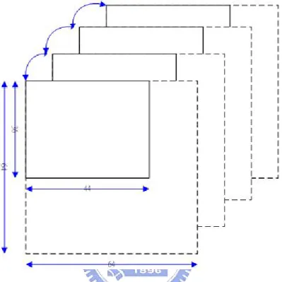
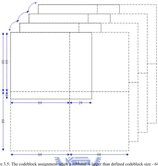
A subband area, which exceeds 64x64, is divided into several codeblocks. The sizes of codeblocks in this subband are 64x64, 8x64, 64x24 and 8x24 as shown in Figure 3.5.
Figure 3.5: The codeblock assignment when a subband is larger than defined codeblock size - 64x64.
3.6.2 Zero coding, Sign coding and Magnitude Refinement
After codeblock assignment, the coefficients are parted into sign data and absolute value. The absolute value of coefficients on a codeblock is decomposed into several bit-plane levels and the sign value is separated on a plane.
The first nonzero bit-pane of the coefficients, i.e. not yet significant in previous bit-plane, are coded by zero coding. If the coefficients become significant at current bit-plane, the corresponded sign data is also coded by sign coding. Magnitude refinement is used to code the new information of the coefficients, which have been
bit-plane decomposition.
Figure 3.6: An example of bit-plane decomposition and coding method. The scanning order is from most significant bitplane to less significant bitplane.
Zero coding: When a coefficient is not yet significant in previous bit-plane, this
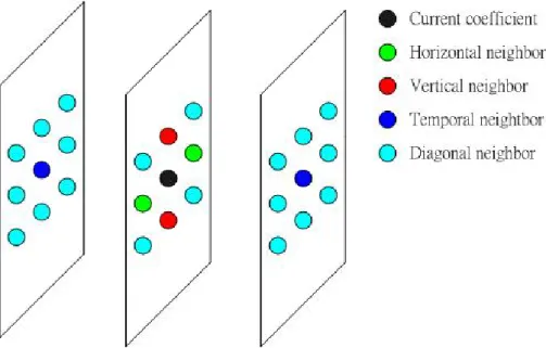
operation is used to code the new information, whether the new information shows this coefficient becomes significant or not. The context model considers not only on spatial neighborhoods but also on temporal correlations. That’s why this entropy coding method named “3D.” Figure 3.7 shows the neighbors of the coefficient, which is considered in a context model.
Figure 3.7: The neighbor of the coefficient considered into context model.
For more details, we consider the context model three categories:
Immediate horizontal neighbors. We denote the number of these neighbors, which are significant by h, 0≤h≤2.
Immediate vertical neighbors. We denote the number of these neighbors, which are significant by v, 0≤v≤2.
Immediate temporal neighbors. We denote the number of these neighbors, which are significant by a, 0≤a≤2.
Immediate diagonal neighbors. We denote the number of these neighbors, which are significant by d, 0≤d≤12
The context assignment map of zero coding described in the 68th MPEG contribution [9][11](the document of MSSVC) is different to the map that is realized in MSSVC. We modified the context assignment map from the document version to the realistic MSSVC version. Table 3.2 lists the modified context assignment map. If more than one conditions are satisfied, we select the lowest context number. After context selection, an adaptive context-based arithmetic coder is utilized to code the
Table 3.2: Context assignmetn map of zero coding
Sign coding: If a coefficient becomes significant in the current bit-plane, sign
coding performs to code the sign of the coefficient after zero coding. There are also a kind of context model and context-based arithmetic coders for sign coding to code the symbol decided by the context model. In order to describe the context module, two variables, σ[i,j,k] and χ[i,j,k], are defined.
σ[i,j,k]: A binary-valued state variable. This value is initialed to 0. If a coefficient of a code block at position [i,j,k] becomes significant, σ[i,j,k] is set to 1.
χ[i,j,k]: The sign of the coefficient of a code block at position [i,j,k]. When the coefficient is positive, the value is 0. On the other hand, if the coefficient is positive, the value is set to 1.
Next, three quantities, h, v and a are defined:
h=min{1, max{-1, σ[i-1,j,k] × (1-2χ[i-1,j,k])+ σ[i+1,j,k]×(1-2χ[i+1,j,k])}}
v=min{1, max{-1, σ[i,j-1,k] × (1-2χ[i,j-1,k])+ σ[i,j+1,k] × (1-2χ[i,j+1,k])}}
a=min{1, max{-1, σ[i,j,k-1] × (1-2χ[i,j,k-1])+ σ[i,j,k+1] × (1-2χ[i,j,k+1])}}
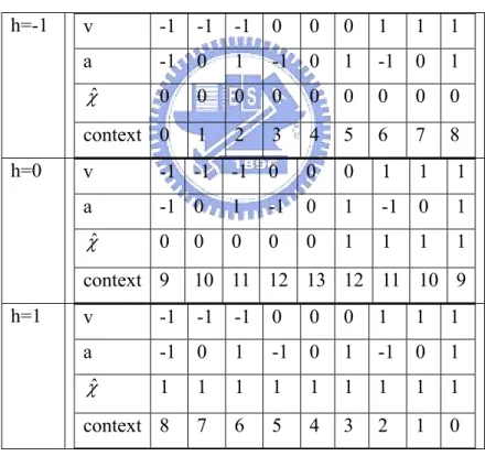
The context module of sign coding is listed in Table 3.3. We have to note thatχˆ means the sign prediction of the coefficient according to its neighbor. Adaptive context-based arithmetic coders finally code the symbol, χ XORχˆ .
Table 3.3: Context assignment map of sign coding
h=-1 v -1 -1 -1 0 0 0 1 1 1 a -1 0 1 -1 0 1 -1 0 1 χˆ 0 0 0 0 0 0 0 0 0 context 0 1 2 3 4 5 6 7 8 h=0 v -1 -1 -1 0 0 0 1 1 1 a -1 0 1 -1 0 1 -1 0 1 χˆ 0 0 0 0 0 1 1 1 1 context 9 10 11 12 13 12 11 10 9 h=1 v -1 -1 -1 0 0 0 1 1 1 a -1 0 1 -1 0 1 -1 0 1 χˆ 1 1 1 1 1 1 1 1 1 context 8 7 6 5 4 3 2 1 0
Magnitude Refinement: If the coefficient has been significant in previous bit-plane,
magnitude refinement is used to code the new information of the coefficient. There are three contexts in this operation. When MR is first performed on the coefficient,
at least one significant neighbor, the context is 1. For the rest conditions, the context is 2.
3.6.3 Significant Propagation Pass, Magnitude Refinement
Pass and Normalization Pass
In section 3.4.2, we illustrated the coding method for a coefficient, but we didn’t give a broad view of how to process all coefficients in a codeblock. In this section, we describe three coding passes. The three coding passes classify the coefficients into three categories and ZC, SC and MR are applied in each category.
After codeblock partition, bit-plane coding is used to code the coefficients in the codeblock. For each bit-plane, three passes process a “fractional bit-plane” in turn and scanning order is i-direction first, then j-direction and k-direction. These passes are described here.
Significant Propagation Pass: The coefficients, not significant in previous
bit-plane but having significant neighbor, are process in this pass. ZC is used to code the value of coefficients in the current bit-plane. If a coefficient becomes significant, SC is performed to code the sign corresponding to the coefficient in the meantime.
Magnitude Refinement Pass: The coefficients, already significant in previous
bit-plane, are coded in this pass. MR coding is used in this pass.
Normalization Pass: The coefficients, not processed in previous two passes, are
coded in this pass. The coefficients entering this pass are not yet significant and don’t have preferred neighborhood. ZC is used and SC is also performed if the coefficient becomes significant.
3.7 SNR/Rate, Spatial and Temporal Scalability
There are mainly three parameters affect the video viewing quality (1) resolution, (2) frame rate, (3) distortion of a picture. The feature of scalability video coding is the ability to achieve the three categories. In this section, we will describe the methods of to achieve three scalabilities.
3.7.1 SNR/Rate Scalability
As describe before, a video sequence is divided into several GOP(group of pictures). The number of frames in a GOP is according to the temporal decomposition level. For example, if temporal decomposition level is p, the GOP size is 2^p. The bit
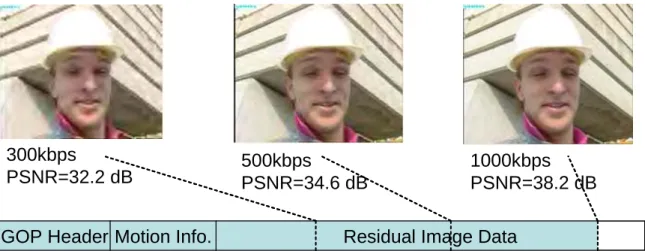
stream after encoding is also arranged according to GOPs in a video sequence. The bit stream in each GOP contains (1) GOP header, (2) motion information and (3) residual image data. Figure 3.8 shows the arrangement of encoded bit stream.
GOP Header Motion Information Data Residual Image Data
Video
Header GOP GOP …… GOP
Figure 3.8: the arrangement of encoded bit stream
Residual image data satisfies the embedded structure and is arranged according to the importance of data. The information of how many bits are used in each bit-plane of a codeblock is recorded. These records are the truncation points during
image data and the truncation positions are right on the truncation points. With the increasing of residual image data, the quality of video sequence is also increased. Figure 3.9 shows the SNR/rate scalability by truncating residual information.
GOP Header Motion Info. Residual Image Data
GOP Header Motion Info. Residual Image Data
300kbps
PSNR=32.2 dB 500kbpsPSNR=34.6 dB 1000kbpsPSNR=38.2 dB
Figure 3.9: SNR/rate scalability can be achieved by truncating the embedded bit-stream. The PSNR performance is increased when bit-rate increase.
3.7.2 Spatial Scalability
When 2D wavelet transform is performed, the lowest frequency represents the lowest resolution frame. As shown in Figure 3.10, adding the information of the HL, LH and HH band, the larger resolution frame, QCIF resolution, can be reconstructed by inverse transform. When the data of LHH, HHL and HHH is added, the resolution of original frame can be reconstructed.
28 8 352 176 14 4 72 88 44 36 HL LH HH HHL LHH HHH LL
Figure 3.10: An example of resolution increasing by 2D wavelet transform
3.7.3 Temporal Scalability
Assume the frame rate of a original video sequence is 30 frames/second. When the receiver request a video sequence at 7.5 frames/second, the requirement can be satisfied with the temporal decomposition structure described in Figure 3.2. If 7.5 frames/second is needed, it only has to package enough information from the fourth temporal level to the third temporal level to the receiver. With this information, the receiver can reconstruct four temporal low frequency frames in second temporal level. After normalization, the four low frequency frames compose the video sequence in 7.5 frames/second within a GOP. By the similar reconstructing method, the
Chapter 4
SB-Reach Method
4.1 Introduction
In the SVC Core Experiment software, the 3D EBCOT entropy coding procedure is used after the MCTF and the spatial transform. We observe that high-energy
wavelet coefficients often cluster together. Inspired by [5][10], we propose a modified coding procedure as described in Section 4.2.1 to save coding bits. Essentially, we construct another layer that records the bit-plane locations ofthe Significant Bits (SB) of all coefficients. We observe bit savings of this technique in our simulation;
4.2 Proposed Entropy Coding Scheme
4.2.1 SB-Reach Method
In the core experiment software, MSSVC, the coefficients are coded by the 3D EBCOT process after the temporal and the spatial subband transforms. Each subband after wavelet transform is partitioned into several codeblocks; then, the entropy coding module encodes these codeblocks. According to the coefficient values in a codeblock, a number of bit-planes are generated, and three coding passes, Significant propagation pass, Magnitude Refinement pass and Normalization pass, are applied to these bit planes sequentially.
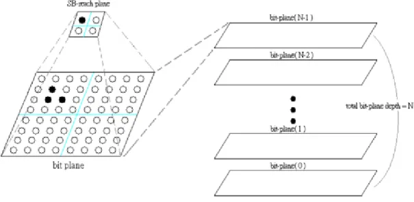
Initially, all wavelet coefficients are “insignificant”. A coefficient becomes “significant” when its non-zero bit is first found. The first non-zero bit will thus be called Significant Bit (SB) (of a coefficient). For each bit plane, we construct another binary bit plane – so-called SB-reach plane. As shown in Figure 4.1, a single sample in the SB-reach plane represents a square mapping block of n by n coefficients. Figure 4.2 shows different size of square mapping block. The size of the SB-reach plane thus decreases as its representing mapping block becomes larger and same square mapping block size is applied for all-bitplanes within defined SB-reach depth in a coding block. By the way, in MSSVC, the size of codeblock is usually 64 by 64, so the size of
square mapping block is at most 32 by 32. The binary sample on an SB-reach plane is set to 1, if its square mapping block contains one or more significant coefficients. On the other hand, if the binary sample on the SB-reach plane is 0, it means that all its associated bits in the coefficient bit plane are zero.
Figure 4.1: One binary sample on the SB-reach plane is associated with 4x4 mapping block bits
Figure 4.2: Examples of square mapping block of n by n coefficients on a bitplane
In this modified coding process, we first construct all the SB-reach bit planes up to the selected “SB-reach depth” as shown in Figure 4.3. Each SB-reach bit plane is associated with one bit plane of the original coefficients. We first encode an SB-reach bit plane before encoding its associated coefficient bit plane using the MSSVC procedure. In encoding an SB-reach plane, we perform the Significant Propagation Pass and the Normalization Pass following the scanning order in MSSVC. If a sample
is classified significant in a previous SB-reach plane, it must be a “1” bit in the current SB-reach plane and thus is not coded. After coding one SB-reach plane, we code its associated coefficient bit-plane. The coefficients on the bit plane are not coded, if its corresponding SB-reach plane bit is zero (insignificant). If a bit on the SB-reach plane is 1, and then its associated coefficient mapping block bits are coded in the order shown in Figure 4.4. We perform three coding passes as the original CES does on these coefficient bits.
Figure 4.4: The encoding process of the SB-reach plane and its associated coefficient bit-plane
With the method described above, we try all combinations of mapping block size and SB-reach depth, and we then compare the resulting coded bits of all combinations. The best combination of mapping block size and SB-reach depth is retained and
coded.
4.2.2 Syntax and Architecture Change
On the top of the core experiment software, we changed some syntax and
decoding procedure as follows. We add the SB-reach plane architecture to the original 3D EBCOT. The information for the mapping block size, the SB-reach plane depth, and the SB-reach planes is added to the original syntax as shown in Figure 4.5.
Figure 4.5: Changes between the original and the proposed syntax
4.3 Coding Procedure
4.3.1 Definition
Here are some definitions in the newly added terms.
SB-reach enable: One bit per coding block represents the SB-reach coding is enabled. “0” = no SB-reach coding; “1” = SB-reach coding enabled.
Mapping_blk_size: The mapping block size information is defined in Figure 4.2. Bit pattern “00” = size 4x4; “01” = 8x8; “10” = 16x16; and “11” = 32x32. SB-reach depth: The depth of SB-reach planes. Bit pattern “00” = depth 2; “01”
= depth 3; “10” = depth 4; and “11” = depth 5.
SB_plane: Record SB-reach bits of the corresponding bit-plane m_nBitDepth: The depth of a codeblock
4.3.2 Coding steps
1. Initial:
SB_plane_old are set to zero. SB_ETA are set to zero. SB_plane_sigma are set to zero. 2. for Mapping_blk_size=n:0
if Mapping_blk_size is zero then the coding process about SB_plane is skipped for y= min of SB-reach depth:max of SB-reach depth
for x= m_nBitDepth-1 : 0 if( x >= m_nBitDepth - y )
GenerateSBplane(x , Mapping_blk_size); CodeSBplane(Mapping_blk_size);
Else
Set all of the SB_plane to 1. Code_Bit_plane();
Set all of SB_ETA to zero;
Pseudo Code
GenerateSBplane(x , Mapping_blk_size ){ For each (i ,j ,k)
SB_plane(Mapping_blk_size, i, j, k) set to “1”, if one of the SB of the correspond coefficients has been reached on the bit-plane(x),
SB_plane_old(Mapping_blk_size, i, j, k) =
SB_plane(Mapping_blk_size, i, j,k) XOR SB_plane_old(Mapping_blk_size, i, j, k) }
CodeSBplane(Mapping_blk_size){ for each (i, j, k)
SignificancePropagationPass_SB (Mapping_blk_size, i, j, k) NormalizationPass_SB(Mapping_blk_size, i, j, k) Set all of SB_ETA to zero.
}
if(SB_ETA(Mapping_blk_size , i , j , k) = 0 )
if( SB_plane_old(Mapping_blk_size, i, j, k)=0 )
if(SB_plane_sigma(Mapping_blk_size, i, j, k)=0 && HasPreferredNeighbor) code SB_plane(Mapping_blk_size, i, j, k); if SB_plane(Mapping_blk_size, i, j, k) is 1 SB_plane_sigma(Mapping_blk_size, i, j, k) set to 1. set SB_ETA(Mapping_blk_size, i, j, k) = 1; } NormalizationPass_SB(Mapping_blk_size, i, j, k) { if(SB_ETA(Mapping_blk_size, i, j, k) = 0 ) if( SB_plane_old(Mapping_blk_size, i, j, k)=0 ) code SB_plane(Mapping_blk_size, i, j, k) } Code_Bit_plane(){ For each (i, j, k)
If( SB_plane(Mapping_blk_size, i, j, k)=1 )
All coefficient in the bit plane associated with the SB_plane(Mapping_blk_size, i, j, k) are coded.
}
4.4 Simulation Results
We evaluate the performance of our algorithm by measuring the bitrate savings between the proposed algorithm and the core experiment software. We follow the Core Experiment (CE) specifications to conduct a series of experiments and to test the effectiveness of the proposed algorithm. Eight sequences are tested, namely, CREW, HARBOR, SOCCER, CITY, BUS, FOOTBALL, FOREMAN, and MOBILE, under different spatial, temporal and bitrate test points. Spatial resolutions are QCIF, CIF, and 4CIF, temporal resolutions are 15, 30 and 60 frame/sec, and bitrates vary from 96 kbit/sec to 3 Mbit/sec. The objective image qualities, or the PSNR values, are almost the same between our results and the results from the core experiment software. Besides, the subjective qualities are almost identical. Therefore, we compare the
Some savings in bits with our algorithm are observed.
In Table 4.1 to Table 4.2, the bitrate savings are expressed in percentage. In these tables, each entry is the total bitrate saving accumulated from the 1st bitplane to the current one. For example, the cumulative biplane 2 means the total bits saved for the 1st, 2nd and 3rd bitplanes together. The positive numbers denote bitrate savings, while the negative numbers mean bitrate loss. The LL, LH, HL, and HH bands in these tables are the spatial subbands of all spatial resolutions accumulated.
Table 4.1: Bitrate savings (in percentage) for the FOREMAN and BUS sequences of the H frames at temporal levels 1 and 2.
FOREMAN BUS Cumulative bitplane LL LH HL HH LL LH HL HH 2 -0.05% 0.2% 0.28% 0.14% -1.34% -0.66% -0.68% -0.15% 3 0.66% 0.44% 0.49% 0.36% 0.31% 0.56% 0.29% 0.44% 4 0.44% 0.26% 0.27% 0.22% 0.18% 0.22% 0.17% 0.23%
Table 4.2: Bitrate savings (in percentage) of the H frames at temporal levels 3 and 4. FOREMAN BUS Cumulative bitplane LL LH HL HH LL LH HL HH 2 0.94% 1.11% 0.85% 0.98% -1.18% 0.01% -0.44% 0.14% 3 1.54% 1.21% 1.13% 1.22% 0.3% 0.7% 0.3% 0.7% 4 0.81% 0.66% 0.59% 0.83% 0.27% 0.30% 0.14% 0.37%
Table 4.3: Bitrate savings (in percentage) at the bottommost temporal level. FOREMAN BUS Cumulative bitplane LL LH HL HH LL LH HL HH 2 -0.25% 0.94% 0.59% 0.93% 0.65% 0.01% 0.03% -0.08% 3 0.09% 1.27% 0.99% 1.04% 0.54% 0.42% 0.21% 0.56% 4 0.05% 0.81% 0.67% 0.69% 0.33% 0.18% 0.11% 0.28%
As shown in the simulation results regarding to the output bitrates, our algorithm performs somewhat better than the CE software. In general, we gain more at the cumulative biplane 3. Particularly, the HH bands at higher temporal levels perform better. Even better results may be obtained by selecting good context and probability models for arithmetic coding. Also, we should tune further the parameter values in our algorithm.
4.5 Appendix A: PSNR value
PSNR old: PSNR value obtained by the original coding procedure (MSSVC.) PSNR new: PSNR value obtained by the modified method.
Test sequences: 4CIF - Crew, Harbour, Soccer and City
CIF – BUS, FOOTBALL, FOREMAN and MOBILE
Table 4.4 : PSNR of CREW
PSNR new PSNR old width height frames/s Kbit/s
Y U V total Y U V total
176 144 15.0 96 31.93 35.51 33.97 32.87 31.94 35.49 33.95 32.87 176 144 15.0 192 34.18 38.07 36.41 35.2 34.19 38.13 36.43 35.22 352 288 30.0 384 33.36 37.49 36.04 34.49 33.35 37.47 36.09 34.49
704 576 30.0 1500 35.8 39.61 39.63 37.08 35.80 39.58 39.61 37.06 704 576 60.0 3000 36.88 40.5 41 38.17 36.87 40.48 40.98 38.16
Table 4.5: PSNR of HARBOUR
PSNR new PSNR old width height frames/s Kbit/s
Y U V total Y U V total 176 144 15.0 96 27.61 38.75 39.22 31.4 27.62 38.78 39.27 31.42 176 144 15.0 192 29.22 40.84 43.23 33.49 29.22 40.86 43.23 33.49 352 288 30.0 384 28.87 39.46 41.56 32.75 28.87 39.48 41.61 32.76 352 288 30.0 750 30.85 41.15 43.01 34.59 30.85 41.16 43.01 34.59 704 576 30.0 1500 32.37 41.25 43.21 35.65 32.37 41.25 43.21 35.65 704 576 60.0 3000 34.42 43.04 45.19 37.65 34.42 43.04 45.20 37.65 Table 4.6: PSNR of SOCCER PSNR new PSNR old width height frames/s Kbit/s
Y U V total Y U V total 176 144 15.0 96 31.53 37.94 39.86 33.98 31.53 37.86 39.88 33.98 176 144 15.0 192 33.38 40.24 41.62 35.9 33.40 40.21 41.64 35.91 352 288 30.0 384 32.53 39.59 41.11 35.14 32.53 39.59 41.14 35.14 352 288 30.0 750 34.52 41.43 43.21 37.12 34.50 41.44 43.20 37.11 704 576 30.0 1500 35.15 41.61 43.44 37.61 35.12 41.61 43.46 37.59 704 576 60.0 3000 36.98 43.22 45 39.35 36.95 43.22 44.96 39.33 Table 4.7: PSNR of CITY PSNR new PSNR old width height frames/s Kbit/s
Y U V total Y U V total
176 144 15.0 64 30.8 40.14 40.88 34.03 30.80 40.14 40.88 34.03 176 144 15.0 128 33.5 41.77 43.66 36.57 33.50 41.77 43.69 36.57 352 288 30.0 256 30.55 41.18 42.82 34.36 30.54 41.07 42.83 34.36 352 288 30.0 512 32.98 41.99 43.61 36.25 32.98 42.01 43.62 36.26
704 576 30.0 1024 32.9 41.59 43.73 36.16 32.90 41.63 43.73 36.16 704 576 60.0 2048 35.07 43.17 45.06 38.08 35.06 43.15 45.06 38.08
Table 4.8:PSNR of BUS
PSNR new PSNR old width height frames/s Kbit/s
Y U V total Y U V total 176 144 7.5 64 24.62 36.69 37.04 28.7 24.63 36.69 37.04 28.71 176 144 15.0 96 25.19 36.95 37.89 29.27 25.19 36.88 37.90 29.26 352 288 15.0 192 27.47 36.97 37.7 30.76 27.47 37.00 37.70 30.76 352 288 15.0 384 30.44 38.6 39.87 33.37 30.44 38.59 39.89 33.37 352 288 30.0 512 30.85 39.16 40.47 33.84 30.85 39.11 40.47 33.83 Table 4.9: PSNR of FOOTBALL PSNR new PSNR old width height frames/s Kbit/s
Y U V total Y U V total 176 144 7.5 128 28.48 33.81 36.69 30.74 28.47 33.81 36.64 30.72 176 144 15.0 192 28.1 33.28 36.48 30.36 28.09 33.27 36.39 30.34 352 288 15.0 384 31.19 34.95 37.31 32.84 31.17 34.96 37.29 32.82 352 288 15.0 512 32.57 36.08 38.23 34.1 32.52 36.06 38.23 34.06 352 288 30.0 1024 34.05 37.44 39.46 35.52 34.01 37.44 3947 35.49 Table 4.10: PSNR of FOREMAN PSNR new PSNR old width height frames/s Kbit/s
Y U V total Y U V total 176 144 7.5 32 28.97 37.11 36.91 31.65 28.97 37.20 36.90 31.67 176 144 15.0 48 29.38 37.56 37.74 32.14 29.39 37.23 37.67 32.08 352 288 15.0 96 30.97 37.46 38.06 33.23 30.96 37.45 38.09 33.23 352 288 15.0 192 33.69 39.27 40.35 35.73 33.66 39.28 40.33 35.71 352 288 30.0 256 34.24 39.64 40.91 36.25 34.23 39.62 40.85 36.23
Table 4.11: PSNR of MOBILE
PSNR new PSNR old width height frames/s Kbit/s
Y U V total Y U V total 176 144 7.5 48 22.54 27.47 26.37 24 22.54 27.47 26.51 24.02 176 144 15.0 64 23.08 28.23 27.31 24.64 23.08 28.24 27.29 24.64 352 288 15.0 128 23.8 28.48 28.04 25.29 23.80 2853 28.10 25.3 352 288 15.0 256 26.94 31.37 30.76 28.32 26.95 31.38 30.77 28.32 352 288 30.0 384 28.57 32.74 32.39 29.9 28.57 32.74 32.35 29.9
4.6 Appendix B: Statistics of SB-Reach Depth and
Block Size
Figure 4.6 to Figure 4.8 show the distributions of the block size and SB-reach depth selected in the tests of BUS, FOOTBALL and FOREMAN. From these statistics, SB-reach disable, 2x2 and 4x4 are the most three popular modes in block size selection. From the SB-reach depth distribution, we can find that 2 is chosen most frequently.
(a) (b)
(a) (b)
Figure 4.7: (a) Block size distribution and (b) SB-reach depth distribution of FOOTBALL
(a) (b)
Figure 4.8 (a) Block size distribution and (b) SB-reach depth distribution of FOREMAN
Table 4.12 shows the bits saving ratio and the overhead ratio of the coded BUS, FOOTBALL and FOREMAN bit streams. The formulas of the bit saving ratio and the overhead ratio is defined in (4.1) and (4.2) and the meaning of a, b and c is are shown by Figure 4.9.
Overhead ratio: b (4.1)
Figure 4.9: ‘a’ the original bitstream without SB-reach method and the bitstream ‘b+c’ is the one with SB-reach method. ‘b’ means the overhead of SB-reach method and ‘c’ means the reduced size bitstream
‘a’ after using SB-reach method.
Table 4.12: Bit saving ratio and overhead ratio for BUS, FOOTBALL and FOREMAN decrease ratio(%) overhead ratio(%)
BUS 0.47 0.3
FOOTBALL 1.31 0.79
Chapter 5
Directional Multiresolution
Transform
5.1. Motivation
In an image and video coding scheme, the spatial transform plays an important role. The image data is transformed to frequency domain by a spatial transform. For typical image, the energy is concentrated to some frequency bands, usually lower frequency bands, and due to the energy compaction property, the compression
efficiency can be improved. There are a few popular spatial transforms used for image compression, such as FFT, KLT, DCT and wavelet transform. However, for the reason of performance and realization, most image or video coding systems adopt DCT and
wavelet transform. 2D-DCT is adopted as the spatial transform module by JPEG, MPEG-1, MPEG-2 and H.264. In JPEG2000 and interframe wavelet coding schemes, the wavelet transform is used.
Wavelets are claimed to be more efficient to represent point abrupt changes and singularities. Because of its good approximation performance in one dimension, wavelets are used in signal processing very frequently. However, in two dimensions, the performance is not as good as in the one dimension. 2D separable wavelets are well adapted to point-singularities, but poor in line- or curve-singularities. In the past decade, Candes and Donoho [12] pioneered a new representation, which is named curvelet to approximate the behavior of 2D smooth functions. Inspired by curvelet, Minh N. Do [13] proposed contourlets to build a new image representation. We will describe this method and apply contourlet to image coding in the fallowing sections.
5.2 Contourlet
Contourlets proposed by Do combine the good properties of curvelets and subband decomposition. It mainly decomposes image in two steps: (1) global
multiscale transforms and (2) local directional transforms. The first step is doing edge detection and applying a wavelet-like transform. In the second step, local directional transforms are used to cover contour segments.
In practice, Do suggests a double filter bank approach. His pyramidal directional filter bank consists of the Laplacian pyramid and the directional filter banks. As shown in Figure 5.1, The Laplacian pyramid decomposes an image into a lower frequency band with 1/4 scale of original data and a higher frequency band. The higher frequency frame is processed further by a directional filter bank, which can have 4, 8 and 16 bands. The lower frequency band can be remained or it can be
further decomposed into low-pass and high-pass bands. Laplacian pyramid is used to cover the point discontinuities and the directional filter bank is used to represent line-segment structures. Thus, the contourlet provides multiresolution decomposition and directional decomposition for an image. Because the contourlet uses the
Laplacian pyramid, it contains redundancy factor up to 1.33, and is not critically sampled.
Figure 5.1: Block diagram of Pyramidal directional filter bank. Multiscale decomposition is at the first stage. Down sampling is applied on the lower frequency band and higher frequency band is followed
by a directional filter bank.
In the next two sections, we describe the design of Laplacian pyramid (LP) and directional filter bank (DFB).
5.3 Laplacian Pyramid
Laplacian pyramid, which is proposed by Burt and Adelson[14], is used to achieve multiscale decomposition. Once Laplacian pyramid is applied, the low-pass image is generated from original image, and then down sampled. The difference of the original image and the predicted image produced from the low-pass image produces
frame of the original image can be then generated.
LP decomposition introduces an over sampling with a ratio of 1.33. On the other hand, wavelet scheme is critically sampling. Intuitively, we see the drawback of LP decomposition may influence coding efficiency. However, the LP decomposition does not have “scrambled” frequency, which happens in the wavelet filter bank. This situation appears when high-pass signal, which is down sampled, is folded back into the low frequency band, and cause its spectrum being reflected (see Figure 5.2). LP decomposition only down sample the low-pass channel and “Scrambled” frequency is avoided.
Highpass(HP)
Downsampled HP
Figure 5.2: Illustration of the “ frequency scrambling.” Upper: spectrum after high-pass filtering. Lower: spectrum after high-pass filtering and downsampling. We can see that the high-pass spectrum is
folded back into the low frequency region.
The architecture of LP is shown in Figure 5.3. H and G are orthogonal filters. X is the input image. And C is the coarse version of X and D is the difference between the original image and the reconstruction of C.
M M H G + -X C D P
Figure 5.3: The analysis side of LP scheme. C is the coarse version of original image and D is the difference between C and input X.
The corresponding synthesis side has two input data - C and D. C is up sampled and then filtered by G. Its output is added by D. The final reconstruction X is then generated (Figure 5.4). M G + -C D X'
Figure 5.4: The synthesis side of the LP scheme. X’ is the reconstructed image.
In realization, the two filters, H and G., have to be selected. We use the 9/7 filters for the LP structure. The coefficients of 9/7 filters are shown in Table 5.1[15].
Table 5.1: 9/7 filter taps
h[n] g[n]
0.037829 -0.064539 -0.023849 -0.040690
-0.110624 0.418092 0.377403 0.788485 0.852699 0.418092 0.377403 -0.040690 -0.110624 -0.064539 -0.023849 0.037829
5.4 Directional Filter Bank
A 2-D Directional filter bank (DFB) is proposed by Bamberger and Smith [16] in 1992. DFB basically partitions the spectrum of 2-D data into wedge-shaped frequency regions and each partition region corresponds to a subband. In realization, a tree structure is used to implement DFB. The number of partition region depends on the level of tree structure realization. For example (Figure 5.5), if the level of tree structure is n, wedge-shaped frequency partitions are generated in frequency domain. 2n 0 2 3 4 7 0 1 1 2 3 4 5 5 6 6 7
ω
2ω
1 (π,π
) (-π,-π
)The construction of DFB involves the QFB’s and fan filters. QFB (quincunx filter bank) is shown in Figure 5.6.
H0 H1 F0 F1 Q0 Q0 Q0 Q0 X X'
Figure 5.6: QFB with sub-lattice sampling Q and fan filters. This also forms the first level of DFB with two directions.
In current case, Q can only be Q0 and Q1, which represents two-dimensional quincunx sub-lattice as shown in Figure 5.7. That is, Q0 and Q1 are applied to the coordinate indices
( )
0 1 1 -1 1 1 , 5.1 1 1 -1 1 Q =⎛⎜ ⎞⎟ Q =⎛⎜ ⎞⎟ ⎝ ⎠ ⎝ ⎠Figure 5.7: Quincunx sampling lattice
With the expansion of the QFB’s, the tree structure become larger and the directions of DFB also increase. In the fallowing discussion, we will use 4-direction and 8-direction DFB’s in our image coding process.
5.4.1 Fan Filter Design
The fan filters are the key components of DFB. In this section, we will describe how to design these filters by using the biorthogonal fan filters designed by Phoong et al. [17].
To obtain the fan filter, diamond-shaped filters are first designed and then modulate the diamond-shaped filters to the fan filters. At first an all pass filter is first established by (5.2) in one dimension. We use the coefficients listed in Table 5.2 (Phoong[17]) as the base of our filter design. The function is derived using {Vk} according to (5.2). In this case, N1 is 6 and theβ
( )
z is 12-taps type II filter.Table 5.2: The base coefficients of 23-45 fan filters
V1 0.630 V2 -0.193 V3 0.0972 V4 -0.0526 V5 0.0272 V6 -0.0144
( )
1(
)
( )
1 1 1 1 5.2 N N k N k k k z v z z β − + − − + = =∑
× +Because the fan filters are 2-dimensional filters, the shape of filter taps is 2-dimensional too. In the Phoong’s thesis, the diamond-shaped filter is the goal of the design. Figure 5.8 shows the ideal diamond-shaped filter.
Ω1 Ω0 π -π ω1 ω0 π -π
Figure 5.8: Ideal diamond-shaped filter
The analysis and synthesis diamond-shaped filters are formed by (5.3).When β(z) is
replaced by β( 1), the 1-dimensional case is turned into 2-dimensional. 0 1 z z−
(
)
(
)
(
)
(
)
(
)
(
) (
)
(
)
(
)
(
)
(
)
2 1 1 0 0 0 1 0 1 0 0 1 1 4 1 1 0 1 0 1 0 1 0 0 1 0 0 0 1 1 0 1 1 0 1 0 0 1 , 2 , , (5.3) , , , , N N z z z z z z H z z H z z z z z z H z z z F z z H z z F z z H z z β β β β − − − − − + + = = − + = − − − = − −With the 6 coefficients of base taps, analysis filters, H0 and H1, have 23x23 and 45x45 2D taps areas. Also, the distribution of taps has the diamond shape. Figure 5.9 shows the impulse response (coefficients) of H0( ) and Figure 5.10 shows the spectrum of the designed H0( ).
0, 1
z z
0, 1
Figure 5.9: H0(z z0, 1) designed with 6 base taps.
Figure 5.10: The spectrum of H0( ). The spectrum is FFT shifted. The value 0 and 1on the axis
represent -π and π. The value 0.5 means frequency value 0.
0, 1
When the diamond-shaped filter has been designed, the next step is to generate the fan filters. Fan filters can be viewed as the modulated diamond-shaped filter. The spectrum of the fan filters is that of the diamond-shaped filter with frequency shifted by –π or π along the X or Y axis. To shift spectrum by –π or π, the modulation operation is applied (5.4).
[ ]
(
0)
(
0)
(
0)
(
1 1 cos 2 5.4 2 d 2 d X nT πnf T ↔ X f − f + X f + f)
In this case, “ f ”, the frequency shift value, is set to be π. The period “T” is set to 0
be 1
2π . The time domain formula can thus be rewritten toX nT
[ ]
cos(
nπ)
. The modulation function cos n(
π)
is in fact a sequence of interleaved +1 and –1. We multiply the modulation sequence to the taps of the analysis and synthesis diamond-shaped filters. Figure 5.11 shows the spectrum of the analysis diamond-shaped filter - H0(z z0, 1) after frequency shifted byπalone Y axis1
The input and the output energy levels of the 23-45 fan filters should be the same. The DC value of H0( ) and F1( ) designed is 0.5 (DC value equals sum of total tap values.). On the other hand, the DC value of H1( ) and F0( ) is 1. The DC levels of signals after passing through two analysis filters are not equal, but the DC value of each analysis and synthesis pair is the same, 0.5*1. Figure 5.12 illustrates DC response of each filter in this structure.
0, 1 z z z z0, 0, 1 z z z z0, 1 The DC value of H0(Z0,Z1) is 0.5 The DC value of H0(Z0,Z1) is 1 The DC value of F0(Z0,Z1) is 1 The DC value of F1(Z0,Z1) is 0.5 Y0 Y1 Total DC level is 0.5 X X' Analysis Synthesis
Figure 5.12: Illustration of DC level in DFB. The DC level of Y0 is half of Y1 because of the different DC levels of H0(z z0, 1) and H1(z z0, 1)
We have to modify the DC levels of the fan filters to produce equal DC levels so that the total system has equal DC responses. The simplest way to achieve this goal is to modify the DC value response of H0( ) and F1( ) from 0.5 to 1. Thus, the value of total taps should be multiplied by 2. With this, the signal after passing each analysis filter bank is at the same DC level and the DC response of total system are 1 after adjustment.
0,