由二維紋理形成具有向量場控制的實體紋理合成

(1)

國

立

交

通

大

學

多媒體工程研究所

碩

士

論

文

由二維紋理形成具有向量場控制

的

實

體

紋

理

合

成

Solid Texture Synthesis with Vector Field Control

from a 2D Texture

研究生：林菊穗

指導教授：施仁忠教授

張勤振教授

中

華

民

國

九

十

八

年

六

月

(2)

由二維材質形成具有向量場控制的實體紋理合成

Solid Texture Synthesis with Vector Field Control from a 2D Texture

研究生：林菊穗 Student：Chu-Sui Lin

指導教授：施仁忠教授 Advisor：Dr. Zen-Chung Shih

張勤振教授

.

Dr.Chin-Chen Chang

國立交通大學

多媒體工程研究所

碩士論文

A Thesis

Submitted to Institute of MultimediaEngineering College of Computer Science

National Chiao Tung University in partial Fulfillment of the Requirements

for the Degree of Master

in

Computer Science

June 2009

Hsinchu, Taiwan, Republic of China

(3)

I

由二維紋理形成具有向量場控制的實體紋理合成

Solid Texture Synthesis with Vector Field Control

from a 2D Texture

研究生：林菊穗指導教授：施仁忠教授

.

張勤振教授

國立交通大學多媒體工程研究所

摘要

本論文輸入一張二維紋理來合成實體紋理(solid texture synthesis)。由於二維紋理在三維空間中無法得知足夠的資訊，故本論文利用預先計算好的三維候選點 (3D-candidates)來做實體紋理合成，三維候選點是分別由三個方向(x, y, z)的 5×5 二維切面(2D slices)所構成，而且必須保持三個切面交叉軸(crossbar)的顏色一致性 (color consistency)，接著利用金字塔合成方法(pyramid synthesis method)來完成實體紋理的合成。在合成過程中使用表面向量值(appearance vector)取代傳統只用色彩值 (RGB color value)來做鄰近點比對，有了資料量豐富的表面向量值，我們就可以分別只比對 4 個點來建立 5×5 個點的三平面內的鄰近點(neighborhood)資料，並利用額外的向量場(vector field)來達到紋理控制(texture control)的目的。

(4)

II

Solid Texture Synthesis with Vector Field Control

from a 2D Texture

Student：Chu-Sui Lin Advisor：Dr. Zen-Chung Shih

.

Dr. Chin-Chen Chang

Institute of Multimedia Engineering

National Chiao Tung University

ABASTRACT

In this thesis, we achieve solid texture synthesis from a 2D input texture. Because 2D input texture does not have enough information in 3D space, we introduce a method that using a set of pre-computed 3D-candidates, each being a triple of interleaved 5×5 2D slices from three coordinates. Moreover, our approach can keep the color consistency along the crossbar of the 3D-candidates. Then we can synthesize solid textures by applying pyramid synthesis method. Appearance vectors are used to replace RGB color values. With these information-rich vectors, 4 locations for each coordinate are used to obtain 5×5 slice neighborhoods. Moreover, we introduce our approach for controllable texture synthesis with vector fields.

(5)

III

Acknowledgements

First of all, I would like to thank my advisors, Dr. Zen-Chung Shih and Dr. Chin-Chen Chang, for their supervision and helps in this work. Then I want to thank all the members in Computer Graphics & Virtual Reality Lab for their comments and instructions. Especially two persons, Yu-Ting Tsai and Ya-Lin Su, I want to thank them for their suggestions and helps. Finally, special thanks for my dear family, and this achievement of this work dedicated to them.

(6)

IV

List of Figures

Figure 1.1 System flowchart ... 4

Figure 3.1 Overview of texture data transformation ... 12

Figure 3.2 The process for feature vector generation: ... 12

Figure 3.3 The diagram of 3D-candidate: ... 14

Figure 3.4 Synthesis from one voxel to m×m×m_{solid texture ... 15}

Figure 3.5 Twelve neighbors for N (v) l s : ... 18

Figure 3.6 Three sub-neighbors for each neighbor of voxel v : ... 19

Figure 3.7 The process of forming triple candidates in direction x : ... 21

Figure 4.1 5×5×5 3D vector field with orthogonal axes ... 23

Figure 4.2 5×5×5 3D vector field with a circle pattern on XY plane ... 24

Figure 4.3 Twelve warped neighbors for N~ (v) l s : ... 27

Figure 4.4 Three warped sub-neighbors for warped neighbors of voxel v ... 29

Figure 4.5 The process of forming warped triple candidates in direction x: ... 30

Figure 5.1 5×5×5 3D vector field about circular & emissive control ... 32

Figure 5.2 5×5×5 3D vector field about slant control ... 33

Figure 5.3 5×5×5 3D vector field about zigzag control ... 34

Figure 5.4 5×5×5 3D vector field about 3D slant control... 35

Figure 5.5 Input and result data for case_1 ... 37

Figure 5.6 Anisometric results with circular control for case_1... 38

Figure 5.7 Anisometric results with emissive control for case_1 ... 39

Figure 5.8 Anisometric results with slant control for case_1 ... 40

Figure 5.9 Anisometric results with zigzag control for case_1 ... 41

Figure 5.10 Anisometric results with 3D slant control for case_1 ... 42

(8)

VI

(9)

1

Chapter 1 Introduction

1.1 Motivation

Nowadays, a lot of textures can be synthesized well in 2D. But there is still a lack of techniques in generating 3D textures. There are different kinds of techniques for 3D surface texturing like texture mapping [8, 23, 24], procedural texturing [5, 15] and image-based surface texturing [18, 20, 22]. 3D surface texturing has some undesired problems, so solid texture is introduced to solve this problems.

Texture mapping is the easiest method for 3D surface texturing, but the quality of the results is not good. It may be suffered from some well-know problems such as distortion, discontinuity, and unwanted seams. Procedural texturing can solve the problems of distortion and discontinuity. However, it still has some drawbacks. Procedural texturing models only limit types of textures, such as marble. Furthermore, users may take time to understand and control parameters. The results will be decided the designers. Image-based surface texturing can synthesize more textures, but it can’t handle large structural textures like bricks. When the curvature is too large, it still has distortion and discontinuous problems. Furthermore, image-based surface texturing is non-reusable such that textures generated for one surface cannot be used for other

(10)

2

surfaces.

Solid textures can be used to solve the above problems. By Peachey [14] and Perlin [15], solid textures are blocks of colored points in 3D space to represent real-world materials. Using solid textures, users do not need to find a parameterization for the surface of the object to be textured. Furthermore, solid textures provide texture information inside the entire volume.

Recently, some techniques [3, 4, 11, 16] used three orthogonal slices for neighborhood matching. We take advantage of this idea and present a method for real 3D space texture synthesis from a 2D texture. Moreover, we use vector fields to control the solid texture synthesis. Unlike above methods, we replace 2D k-coherent candidates with 3D-candidates. When we select the best matching candidates, we consider all the three directions instead of each direction independently. We use information-rich appearance vectors for neighborhood matching. The whole process is automatic. The results illustrate that our approach can do well on a wide range of textures.

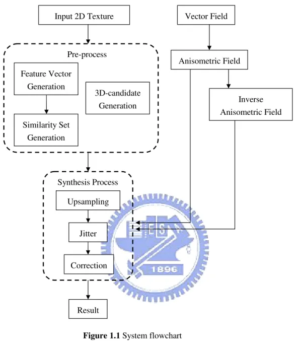
1.2 Overview

The flowchart of our system is shown in Figure 1.1. First, input a 2D texture and repeat the texture thrice as three directional exemplars. In the pre-process, it generates feature vectors, similarity sets, and 3D-candidates for each pixel. For feature vector generation, it captures 5×5 window information and uses principal component analysis (PCA) to decrease the dimensions. For similarity set generation, it finds the three pixels most similar to each pixel. For 3D-candidates generation, it computes a small candidate set from the other two exemplars for each pixel. In the synthesis process, we apply the

(11)

3

pyramid synthesis method [12] to our system. Upsampling, jitter and correction are used at each synthesis level to obtain the results. For anisometric synthesis, vector fields are used to control the synthesis. We input a vector field as the anisometric field and compute the inverse anisometric field. These two fields are used in synthesis process to get the results.

The major contributions of this thesis are as follows: First, we present an approach for synthesizing solid textures from a 2D texture. Using appearance vectors, only 12 locations (4 locations for each direction) are needed to synthesize solid textures. Second, we present a coherent anisometric synthesis method for solid textures according to vector field control.

1.3 Thesis Organization

The rest of this thesis is organized as follows: In Chapter 2, we review related works about texture synthesis with control and solid texture synthesis. In Chapter 3, we present our approach for synthesizing solid textures from a 2D texture. Chapter 4 presents the proposed anisometric synthesis approach for solid textures based on vector field control. Chapter 5 shows the implementation and results. Finally, conclusions and future works are discussed in Chapter 6.

(12)

4

Input 2D Texture Vector Field

Feature Vector Generation Anisometric Field Inverse Anisometric Field Similarity Set Generation Pre-process Upsampling Jitter Synthesis Process Correction Result

Figure 1.1 System flowchart

3D-candidate Generation

(13)

5

Chapter 2 Related Works

In this chapter, we review some recent and representative works.

2.1 Texture Synthesis with Control Mechanism

Ashikhmin [1] presented a texture synthesis algorithm for natural textures. He provided an interactive interface for users to control the texture synthesis process. He introduced an idea of “shifted-candidates” for neighborhood matching and found the best similar candidate. This approach uses a smaller neighborhood to obtain the quality characteristics of a larger neighborhood and maintains the coherence of the results. Users can use painting-style interface to indicate large-scale properties of the texture. Furrhermore, this method is fast and straightforward for the users. But it could not obtain good results if the user’s control does not contain significant amount of high frequency components.

(14)

6

Lefebvre and Hoppe [12] introduced a high-quality and parallel pyramid synthesis algorithm. Their method includes upsampling step to maintain patch coherence, jittering of exemplar coordinates to increase the randomness of the texture, and an order-independent correction step to keep the similarities between synthesized results and input textures. They obtained high-quality and efficient results thanks to the order-independent correction step. It corrects the pixel coordinate for more accurate neighborhood matching and the whole step can be divided into several subpasses to promote performance. However, it still has one drawback: when the features are too large to be captured by small neighborhoods, it could perform poorly. This drawback is also a well-known problem for other neighborhood-based per-pixel synthesis methods.

Lefebvre and Hoppe [13] proposed a structure for exemplar-based texture synthesis with anisometric control. They replaced traditional RGB values with appearance vectors for neighborhood matching. Their appearance space reduces runtime neighborhood vectors from 5×5 grids to only 4 locations, so the synthesis is more efficient, and the quality of results is good because of the information-rich appearance vectors. In addition, they combined their pyramid synthesis with appearance vectors to accelerate neighborhood matching and proposed novel methods for coherent anisometric synthesis which makes arbitrary affine deformation on textures. They presented a convenient way to control textures.

Kwatra et al. [9] introduced a method to control flows on 2D textures and presented an algorithm to perform texture control on 3D surfaces [10]. They proposed a vector advection technique with global texture synthesis to accomplish dynamically changing

(15)

7

fluid surfaces. Users can define fluid velocity field to control the texture results on 3D surfaces. The neighborhood construction step in the process considers orientation coherent with the user-defined velocity field. This method not only makes the synthesized results similar to the input texture, but also keeps temporally coherent. However, it is difficult for users to define an orientation velocity field which is smooth everywhere.

2.2 Solid Texture Synthesis

Jagnow et al. [7] used traditional stereological methods to synthesize 3D solid textures from 2D images. They synthesized solid textures for spherical particles first and then extended the technique to apply to arbitrary-shaped particles. Their approach needs cross-section images to record the distribution of circle sizes on 2D slices, and then builds the relationship of 2D profile density and 3D particle density. Users could use the particle density to add one particle at a time to reconstruct the volume data, so it means the step is manual. This method uses many 2D profiles to construct 3D density for volume results, which are good for marble textures. However, their system is not automatic and only for particle textures.

Chiou and Yang [2] improved the above system to automatic process. They divided the synthesis into two parts: 2D analysis phase and 3D synthesis phase. First, they collected essential statistics to develop a probability model. Then they used this probability model to control the variation in particle size through the 3D synthesis procedure. However, this system inherits the above system so it is only for particle textures.

(16)

8

Qin et al. [16] introduced an image-based solid texturing in terms of basic gray-level aura matrices (BGLAMs) framework. They replaced traditional gray-level histograms with BGLAMs for neighborhood matching. They defined aura matrices from input exemplars and generated a solid texture from multiple view directions. In the volume result, they will only consider the pixels on the three orthogonal slices for

neighborhood matching.The whole system is fully automatic without user interactions.

Furthermore, they can generate reliable results for both stochastic and structural textures. However, it needs large storages for large matrices and the results are not good for color textures.

Kopf et al. [11] provided a solid texture synthesis method from 2D exemplars. They took advantage of 2D texture optimization techniques to do 3D solid texture synthesis and then preserved global statistical properties by histogram matching to achieve optimization. For each voxel, they only considered the neighborhood coherence in three orthogonal slices, and increased the similarity between the solid textures and the exemplar iteratively. Their approach could do well for wide range of textures. But they synthesized the texture with the information on the slices.

Takayama et al. [17] presented a method which fills a model with anisotropic textures. They had some volume textures and defined it how to map to 3D objects. Then they pasted solid texture exemplars repeatedly on the 3D object. Volumetric tensor over the mesh can be set by users, and the texture patches are located according to these fields. This method still has drawbacks. The patch seams became noticeable when using a texture with strong low-frequency components and the blurring artifacts appeared

(17)

9

when using highly structured textures.

Dong et al. [4] introduced a new algorithm to restrict synthesis to a subset of the voxels, while enforcing spatial determinism. They reduced the dependency chain of neighborhood matching, so that each voxel only depended on a small number of other voxels. They synthesized a volume by using pre-computed 3D-candidates, each being a triple of interleaved 2D neighborhoods. These 3D-candidates are selected carefully to form consistent triples. Their approach could generate good results efficiently. However, if the three exemplarsdo not define a coherent 3D volume, the quality of the result will be poor.

2.3 Texture Synthesis and Vector Field

Many patterns are created by interactions between texture elements and surface geometry, so Turk [18] synthesized a texture directly on the surface of the model. An orientation field must be specified over the surface in order to preserve the directional nature of textures. They did this by allowing users to pick the directions at several locations and then interpolating vectors over the rest of the surface.

Ying et al. [22] presented a method that synthesized the texture directly on the surface, rather than synthesizing a texture image and mapping it to the surface. A 2D vector field was used to specify the correspondence between orientation on the surface and orientation in the domain of the example texture. A pair of orthogonal tangent vector fields is used for the purpose. They got one field first, and the second field is computed as the cross-product of the first field and the oriented surface normal.

(18)

10

Taponecco et al. [19] used Markov Random Field (MRF) texture synthesis method to implement 2D vector field visualization. In their approach, they defined a vector field by magnitude and direction. The magnitude could be easily computed using an appropriate norm of the values. Assigning the direction required a projection of the vector onto the image plane, and then the angle of the tangent in the vector field relative to the x-axis is gotten. The magnitude and direction were used to scale and rotate the image.

Wu et al. [21] proposed an approach to directly synthesize texture on arbitrary surface with texture sample. It had a tangential vector field which indicated the desired growing orientation of the texture on the surface. First, users specified tangential vectors at a few seed triangles, and then they interpolated vectors at the remaining triangles to build a tangential vector field. They recursively mapped triangles to texture space until the whole surface is mapped completely based on the vector field.

(19)

11

Chapter 3 Solid Synthesis Process

In this section, we present our approach for synthesizing solid textures from 2D textures. In Section 3.1, we describe feature vectors in appearance space and how we get the feature vectors. Then we use the similarity set to accelerate neighborhood matching in Section 3.2. In Section 3.3, we keep the color coherence of the three orthogonal slices by computing 3D-candidates. We introduce how to apply 2D pyramid texture synthesis to solid texture synthesis in Section 3.4. The upsampling process increases the texture sizes between different levels, that each voxel in parent level generates eight voxels in children level. The jitter step perturbs the textures to achieve deterministic randomness. The last step in pyramid solid synthesis is voexl correction, using neighborhood matching to make the results more similar to the exemplar.

3.1 Feature Vector Generation

(20)

12

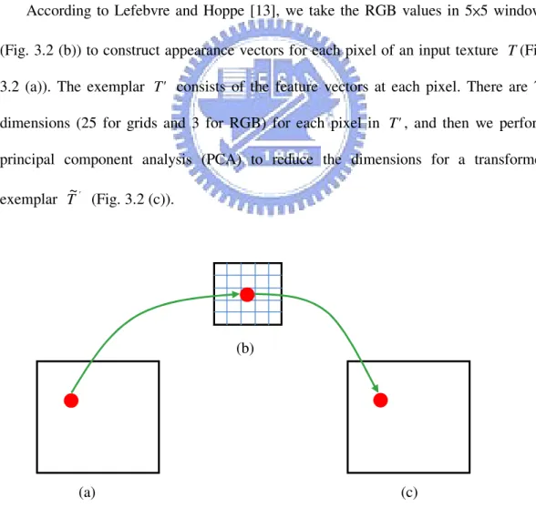
larger neighborhood size and data. Appearance vectors have been proved that they are continuous and low-dimensional for neighborhood matching. Hence, we transform the texture data values in color space into feature vectors in appearance space. As shown in Fig. 3.1, we transform texture data T into appearance space texture data T'.

Figure 3.1 Overview of texture data transformation

According to Lefebvre and Hoppe [13], we take the RGB values in 5×5 windows (Fig. 3.2 (b)) to construct appearance vectors for each pixel of an input texture T(Fig. 3.2 (a)). The exemplar T' consists of the feature vectors at each pixel. There are 75 dimensions (25 for grids and 3 for RGB) for each pixel in T', and then we perform principal component analysis (PCA) to reduce the dimensions for a transformed exemplar _T~'_{(Fig. 3.2 (c)).}

Figure 3.2 The process for feature vector generation: (b)

(21)

13

(a) input texture data T (b) 5×5 windows structure for feature vectors (c) transformed exemplar T~'

3.2 Similarity Set Generation

By the k -coherence search method [24], searching from the candidates can accelerate neighborhood matching because we do not have to search from each pixel in the exemplar for neighborhood matching. Thus, we construct a similarity set to record the candidates similar to each pixel.

Based on the principle of coherence synthesis [1], searching candidates from the

n

n× neighbors of pixel p in the exemplar T can accelerate the synthesis process. Hence, we find the k most similar pixels from the n×n neighbors of pixel p in the transformed exemplar T~' to construct the similarity set C₁l_..._k(p) for pixel p, where

k is a user-defined parameter, and l is the pyramid level, C1l(p)=p. Note that n is a

user-defined parameter to control the window size for coherent synthesis. In the experiments, n is set as 7.

3.3 3D-Candidate Generation

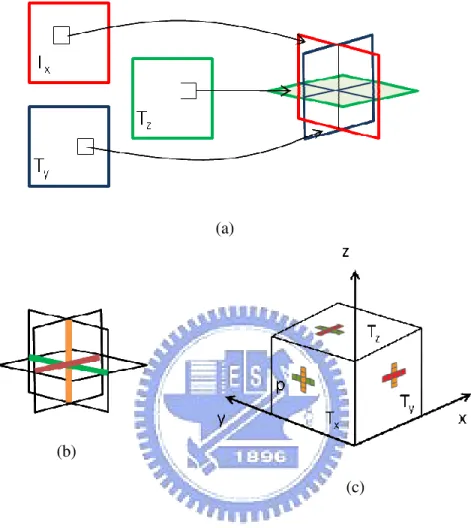
First, we repeat the input texture thrice as three directional exemplarsT_x, T_yand T_z. By Dong et al. [4], we generate a small set of 3D-candidates for each pixel of the three exemplars to build the relation between the three exemplars. The 3D-candidate is by three 5×5 slices (2D neighborhoods) (Fig. 3.3 (a)). It is important that a suitable candidate should be consistent across the crossbar. The crossbar is the strip that is intersected by two slices (Fig. 3.3 (b)). Therefore, we seek to minimize the color

(22)

14

disparity between the strips shared by interleaved slices.

Figure 3.3 The diagram of 3D-candidate:

(a) Three input exemplars Tx, Ty, Tz and a corresponding 3D-candidate.

(b) The crossbars are defined by the three slices. (c) A consistent triple from each exemplar.

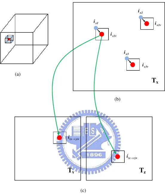
We define the triple to be the three coordinates which is pointed by the center pixel of the three slices. For each pixel of each exemplar, we form triples using the pixel and two neighborhoods from the other two exemplars. We select the triples which have the smaller crossbar error. The 3D-candidate set is composed of these triples. For instance, as shown in Fig. 3.3(c), assuming we want to compute a 3D-candidate set for

(a)

(b)

(23)

15

pixel p in T_x, we first find in T_y the K pixel strips best matching the orange line from

x

T , and in T_z the K pixel strips best matching the green line from T_x. We use the current pixel p as the third coordinate to produce all possible K2 triples, and then order them based on the crossbar error which is the sum of color differences for the three of pixel strips. In the experiments, we keep the 12 best triples as 3D-candidates for each pixel and set a value K as 65.

3.4 Pyramid Solid Texture Synthesis

3.4.1 Pyramid Upsampling

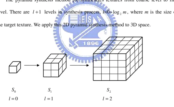
The pyramid synthesis method [6] synthesizes textures from coarse level to fine level. There are l+1 levels in synthesis process, l=0~log₂m, where m is the size of the target texture. We apply this 2D pyramid synthesis method to 3D space.

Figure 3.4 Synthesis from one voxel to m×m×m solid texture

In our approach, we synthesize from one voxel to a m×m×m solid texture, from

L

S

S₀ ~ , where L=log₂m, as shown in Fig. 3.4. We synthesize a volume data S in

which each voxel S

[ ]

v stores three coordinate values, indicatingT , ~_x' T , ~y' ' ~ z T 0 S S1 S2 0 = l l =1 l=2

(24)

16

exemplar’s pixel, respectively. First, we build a voxel and assign value (1,1), (1,1), (1,1) to it as triple coordinates. Then, we upsample the coordinates of parent voxels for next level, assigning each eight children the scaled parent coordinates plus child-dependent offset as

(

mod2, mod2

)

] 2 , 2 , 2 [ ] [ijk S ₁ i j k h j k Sl x l  x+ l            = − ,

(

mod2, mod2

)

] 2 , 2 , 2 [ ] [ijk S ₁ i j k h i k S_l _y _l _y + _l             = ₋ ,

(

mod2, mod2

)

] 2 , 2 , 2 [ ] [ijk S ₁ i j k h i j S_l _z _l _z+ _l             = ₋ , ) (log2 2 m l l h = −

where h denotes the regular output spacing of exemplar coordinates, and _l ijk

means the location of voxel v. S_l[ijk]_x is the new coordinate value at location ijk

within the volume of level l for exemplar T . ~_x' S_l[ijk]_y is the new coordinate value at location ijk within the volume of level l for exemplar T . ~_y' Sl[ijk]z is the new

coordinate value at location ijk within the volume of level l for exemplar T~_z'.

3.4.2 Jitter Method

After upsampling the coordinates, we have to jitter our texture to achieve deterministic randomness. We plus the upsampled coordinates at each level a jitter function value to perturb it. The jitter function J_l(v) is produced by a hash function

[

]

2 2 1 , 1 : ) (v Ζ → − +

(25)

17 ) ( ] [ ] [v S v J v S_l = _l + _l l l l v hH v r J ( )= ( )

3.4.3 Voxel Correction

In order to make the coordinates similar to those in the exemplars T_x, T_y, T_z, we take the jittered results to recreate neighbors. There is a feature value for each pixel after constructing feature vectors. For each voxel v, we collect the feature values of its neighbors to obtain the neighborhood vectors N_s v _x

l( ) , Nsl(v)y, Nsl(v)z for each

direction, respectively. Then, we search the most similar pixel from the transformed exemplars T , ~_x' T , ~_y' T~_z' to make the result similar to the exemplars T_x, T_y, T_z.

In neighborhood matching, we take 4 diagonal locations for voxel v in each direction to obtain the neighborhood vectors N_s v _x

l( ) , Nsl(v)y, Nsl(v)z:                     ± ± = ∆ ∆ + = 1 1 0 ]] [ [ ~ ) ( _x _x' _x _x s v T S v N l                     ± ± = ∆ ∆ + = 1 0 1 ]] [ [ ~ ) ( _y _y' _y _y s v T S v N l                     ± ± = ∆ ∆ + = 0 1 1 ]] [ [ ~ ) ( _z _z' _z _z s v T S v N l

(26)

18

Figure 3.5 Twelve neighbors for N (v)

l

s :

(a) 4 neighbors for N_s v _x

l( ) (b) 4 neighbors for Nsl(v)y

(c) 4 neighbors for N_s v _z

l( )

Based on [13], for N_s v _x

l( ) , we average the voxels nearby voxel v+∆x to

improve convergence without increasing the size of the neighborhood vector N_s v _x

l( ) .

We average the appearance values from 3 synthesized voxels nearby v+∆_x as the new feature value at voxel v+∆_x, and then use the new feature values at 4 diagonal voxel to construct neighborhood vector N_s v _x

l( ) . Also, Nsl(v)y and Nsl(v)z can be done by

the same process. N_s (v; _x)

l ∆ means the averaged feature value at voxel v+∆x .

) ; ( _y

s v

N

l ∆ means the averaged feature value at voxel v+∆y. Nsl(v;∆ means the z)

averaged feature value at voxel v+∆_z.

∑

+∆ +∆′ −∆′ = ∆ _∆′₌ _∆ _∈_Ψ ~[ [ ] ] 3 1 ) ; ( _x _M _,_M _x' _x sl v x xT S v N

{

}

                              ∈ Ψ 1 0 0 0 0 0 0 0 0 , 0 0 0 0 1 0 0 0 0 , 0 0 0 0 0 0 0 0 0 x

∑

+∆ +∆′ −∆′ = ∆ ∆′= ∆ ∈Ψ [ [ ] ] ~ 3 1 ) ; ( _y _M _,_M _y' _y sl v y yT S v N (a) (b) (c)

(27)

19

{

}

                              ∈ Ψ 1 0 0 0 0 0 0 0 0 , 0 0 0 0 0 0 0 0 1 , 0 0 0 0 0 0 0 0 0 y

∑

+∆ +∆′ −∆′ = ∆ _∆′₌ _∆ _∈_Ψ ~[ [ ] ] 3 1 ) ; ( _z _M _,_M _z' _z sl v z zT S v N

{

}

                              ∈ Ψ 0 0 0 0 1 0 0 0 0 , 0 0 0 0 0 0 0 0 1 , 0 0 0 0 0 0 0 0 0 z

Fig. 3.6 shows the locations of 3 synthesized voxels for each neighbor.

Figure 3.6 Three sub-neighbors for each neighbor of voxel v : (a) in N_s v _x

l( ) (b) in Nsl(v)y (c) in Nsl(v)z

We use the similarity sets and coherence synthesis method in the searching process, utilizing the 4 voxels for each direction nearby voxel v . Taking direction x for example, for the neighbor voxel i_x (i_x =1~4), we can get the most similar 3 pixels (i_x₁,i_x₂,i_x₃) in exemplar _{T for voxel}_x i_x from the similarity set. And then we the offset between voxel i_x and voxel v from 3D space to 2D space to infer the

(28)

20

candidates (i_x₁_v,i_x₂_v,i_x₃_v) in exemplar T for voxel v (Fig. 3.7(b)). In order to keep _x

color consistence in three directions, we use the 3D-candidate set to infer the other two coordinates (i₍_x_→_y₎_v , i₍_x_→_z₎_v ) in exemplars T_y and _{T (Fig. 3.7(c)). In addition,}_z directions y , z are done by the same steps.

Now, for each v , we can get a set of triple candidates TC_1..._k_{which point towards}

pixels in exemplars T_x, T_y, T . We compute the neighborhood vectors _z Nsl(TC1...k)x,

y k s TC

N

l( 1... ) , Nsl(TC1...k)z by the averaged feature values from the 4 nearby pixels.

Finally, we sum up the total difference between N_s TC _k _x

l( 1... ) , Nsl(TC1...k)y ,

z k s TC

N

l( 1... ) and Nsl(v)x, Nsl(v)y, Nsl(v)z, then replace the triple coordinate for

(29)

21

Figure 3.7 The process of forming triple candidates in direction x : (a) A voxel v is corrected.

(b) The candidates in exemplar T_x_.

(c) Find the other two candidates in exemplar Ty and Tz.

(a) (b)

T

x

T

y

T

z (c) x1 i x2 i x3 i x1v i x2v i x3v i y)v (x i _→ z)v (x i →

(30)

22

Chapter 4 Anisometric Synthesis Process

In this section, we present the proposed anisometric synthesis approach for solid textures with vector field control. In Section 4.1, we introduce 3D vector fields and how we generate anisometric fields and inverse anisometric fields with the 3D vector fields. In Section 4.2, we introduce the differences between solid synthesis and anisometric synthesis. These different steps are upsampling and correction. The jitter step is the same as it in the solid synthesis process.

4.1 3D Vector Field

We need the user-defined 3D vector fields to implement anisometric solid texture synthesis. We use these 3D vector fields to control the result.

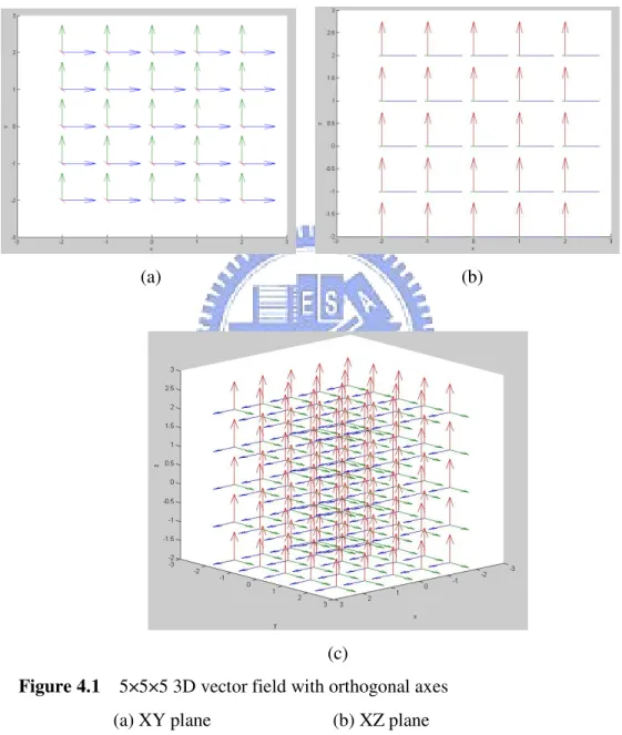
First, we design a 3D space which contains three orthogonal axes at every point, then we use mathematics formulas to control the three axes. Fig. 4.1 shows a 3D vector field with orthogonal axes at each point, and the space size is 5×5×5. We make the three

(31)

23

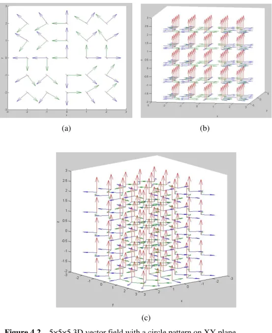
axes various, and expect that the texture results would be changed with the fields. For example, we design a circular field, and there will be a circular pattern on the texture. Fig. 4.2 shows the 3D vector field with a circular pattern on XY plane. The vector field should be the same size as the texture result.

(a) (b)

(c)

Figure 4.1 5×5×5 3D vector field with orthogonal axes

(a) XY plane (b) XZ plane (c) three orthogonal axes at each point

(32)

24

(a) (b)

(c)

Figure 4.2 5×5×5 3D vector field with a circle pattern on XY plane

(a) XY plane (b) and (c) are three axes at each point

For each level, we have to make the anisometric field A and the inverse anisometric field −1

A based on the user-defined 3D vector field. The anisometric field

A is created by downsampling the 3D vector field, and we obtain A_l for each level. Afterward we inverse the A_l to get inverse anisometric field A_l−1 for each level. In anisometrc synthesis process, the upsampling and correction steps will refer to the fields

(33)

25

l

A and A_l−1 at each level.

4.2 Anisometric Solid Texture Synthesis

4.2.1 Pyramid Upsampling

The goal for upsmapling step in anisometric synthesis is the same as it in isometric synthesis. It synthesizes from coarse level to fine level. We upsample the coordinate values of parent voxels for the next level.

The difference is that the child-dependent offset for upsmapling step is dependent on the anisometric field A. The anisometric field A is used to compute the distance for spacing. ) ( ] [ ] [v S 1v h A v S_l _x = _l− −∆_x _x + _l∆_x⋅ _l ) ( ] [ ] [v S ₁ v h A v S_l _y = _l− −∆_y _y + _l∆_y⋅ _l ) ( ] [ ] [v S ₁ v h A v S_l _z = _l− −∆_z _z + _l∆_z⋅ _l ) (log2 2 m l l h = −

{

}

                    −           −           − −                     −           −           − − ∈ ∆ 5 . 0 5 . 0 0 , 5 . 0 5 . 0 0 , 5 . 0 5 . 0 0 , 5 . 0 5 . 0 0 , 5 . 0 5 . 0 0 , 5 . 0 5 . 0 0 , 5 . 0 5 . 0 0 , 5 . 0 5 . 0 0 x

{

}

                    −           −           − −                     −           −           − − ∈ ∆ 5 . 0 0 5 . 0 , 5 . 0 0 5 . 0 , 5 . 0 0 5 . 0 , 5 . 0 0 5 . 0 , 5 . 0 0 5 . 0 , 5 . 0 0 5 . 0 , 5 . 0 0 5 . 0 , 5 . 0 0 5 . 0 y

{

}

                    −           −           − −                     −           −           − − ∈ ∆ 0 5 . 0 5 . 0 , 0 5 . 0 5 . 0 , 0 5 . 0 5 . 0 , 0 5 . 0 5 . 0 , 0 5 . 0 5 . 0 , 0 5 . 0 5 . 0 , 0 5 . 0 5 . 0 , 0 5 . 0 5 . 0 z

where h_l is the regular output spacing of exemplar coordinates. ∆_x means the relative locations for 8 children in direction x , and ∆ , _y ∆_z as well.

(34)

26

4.2.2 Voxel Correction

The goal for correction step is to make the coordinates similar to those in the exemplars T_x, T_y, T_z. For each voxel v , we collect the feature values of warped neighbors by the anisometric field A_l and the inverse anisometric field A_l−1to obtain

x s v

N

l( ) , Nsl(v)y , Nsl(v)z . Then we search the most similar voxel from the

transformed exemplars T~_x', T , ~_y' T~_z' to make the result similar to the exemplars T_x,

y

T , T according to the 3D vector field. _z

Lefebvre and Hoppe [13] presented a method for anisometric synthesis which is able to reproduce arbitrary affine deformations, including shears and non-uniform scales. They only accessed immediate neighbors of pixel p to construct the neighborhood vector N ( p)

l

s . They used the Jacobian field J and the inverse Jacobian field 1 −

J to infer which pixel neighbors to access, and the results will be transformed by the inverse Jacobian field J−1 at the current point. We apply this method to 3D space.

First, we have to know which 4 voxel neighbors in each direction to voxel v. We

use the inverse anisometric field A_l−1 to infer the 4 warped neighbors for voxel v, and

construct the three warped neighborhood vectors N_s v _x

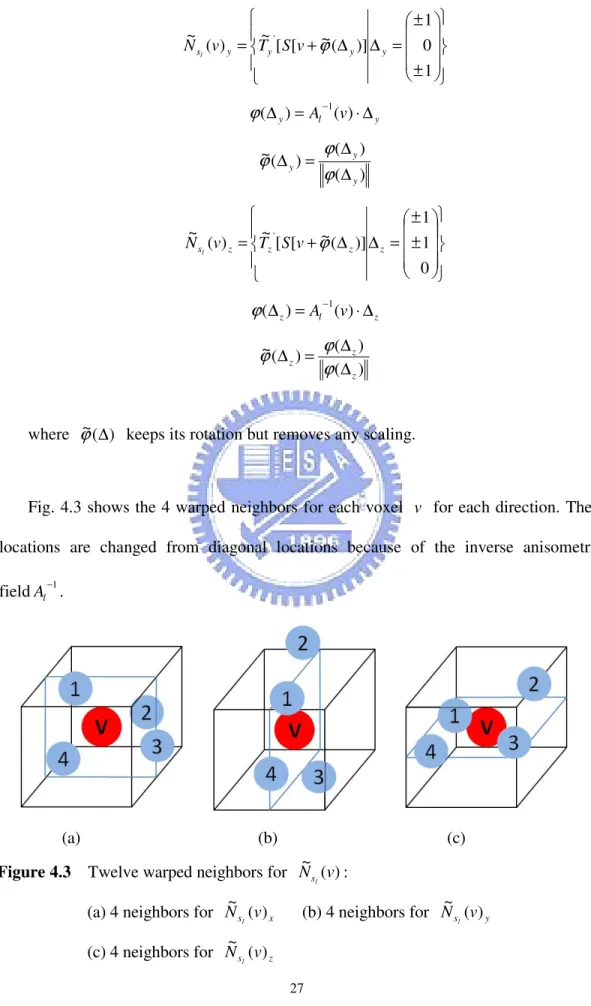
l( ) ~ , N_s v _y l( ) ~ , N_s v _z l( ) ~ :                     ± ± = ∆ ∆ + = 1 1 0 )] ( ~ [ [ ~ ) ( ~ ' x x x x s v T S v N l ϕ x l x =A v ⋅∆ ∆ ) − ( ) ( 1 ϕ ) ( ) ( ) ( ~ x x x ∆ ∆ = ∆ ϕ ϕ ϕ

(35)

27                     ± ± = ∆ ∆ + = 1 0 1 )] ( ~ [ [ ~ ) ( ~ ' y y y y s v T S v N l ϕ y l y = A v ⋅∆ ∆ ) − ( ) ( 1 ϕ ) ( ) ( ) ( ~ y y y ∆ ∆ = ∆ ϕ ϕ ϕ                     ± ± = ∆ ∆ + = 0 1 1 )] ( ~ [ [ ~ ) ( ~ ' z z z z s v T S v N l ϕ z l z =A v ⋅∆ ∆ ) − ( ) ( 1 ϕ ) ( ) ( ) ( ~ z z z ∆ ∆ = ∆ ϕ ϕ ϕ

where ϕ~ ∆( ) keeps its rotation but removes any scaling.

Fig. 4.3 shows the 4 warped neighbors for each voxel v_{for each direction. Their}

locations are changed from diagonal locations because of the inverse anisometric fieldA_l−1.

(a) (b) (c) Figure 4.3 Twelve warped neighbors for N~ (v)

l

s :

(a) 4 neighbors for N_s v _x

l( ) ~ (b) 4 neighbors for N_s v _y l( ) ~ (c) 4 neighbors for N_s v _z l( ) ~

(36)

28

Second, we have to find the 3 synthesized voxels nearby warped neoghborhod voxels of voxel v_{for each direction. Taking direction} x_{for example, we use the}

inverse anisometric field −1

A to infer the 3 synthesized voxels for voxel v+ϕ~(∆_x), and compute the averaged feature value as the new feature value at v+ϕ~(∆_x). Also, directions y , z_{are done by the same process. Fig. 4.4 shows the locations of 3}

warped synthesized voxels for each warped neighbor.

] )] ( ~ ) ( ~ [ [ ~ 3 1 ) ; ( ~ ' ), ( ~ ) ( ~ _x _x _x _x x M M x sl v T S v M N x x + ∆ + ′ ∆ − ∆ = ∆

∑

ϕ′_∆ ₌ϕ _∆ _∈_Ψ ϕ ϕ

{

}

                              ∈ Ψ 1 0 0 0 0 0 0 0 0 , 0 0 0 0 1 0 0 0 0 , 0 0 0 0 0 0 0 0 0 x ] )] ( ~ ) ( ~ [ [ ~ 3 1 ) ; ( ~ ' ), ( ~ ) ( ~ _M _M _y _y _y _y y sl v T S v M N y y y + ∆ + ′ ∆ − ∆ = ∆

∑

ϕ′∆ =ϕ ∆ ∈Ψ ϕ ϕ

{

}

                              ∈ Ψ 1 0 0 0 0 0 0 0 0 , 0 0 0 0 0 0 0 0 1 , 0 0 0 0 0 0 0 0 0 y ] )] ( ~ ) ( ~ [ [ ~ 3 1 ) ; ( ~ ' ), ( ~ ) ( ~ _z _z _z _z z M M z sl v T S v M N z z + ∆ + ′ ∆ − ∆ = ∆

∑

ϕ′_∆ ₌ϕ _∆ _∈_Ψ ϕ ϕ

{

}

                              ∈ Ψ 0 0 0 0 1 0 0 0 0 , 0 0 0 0 0 0 0 0 1 , 0 0 0 0 0 0 0 0 0 z

(37)

29

(a) (b) (c)

Figure 4.4 Three warped sub-neighbors for warped neighbors of voxel v

We utilize the 4 warped voxels for each direction nearby voxel v . Taking direction x_{for example, the warped neighbor voxel} i′_x (i′_x =1~4), we can get the most similar 3 voxels (i′ ,_x₁ i′ ,_x₂ i′ ) in exemplar _x₃ T for voxel x i′ from the similarity set. Then we x

use the warped relationship with the anisometric fields A between voxel i′ and _x

voxel v to infer the candidate voxels (i_x′₁_v,i′_x₂_v,i_x′₃_v) in exemplar T_x for voxel v , as shown in Fig. 4.5(b). We want to keep the color consistence in three directions, so we use the precomputed 3D-candidate set to infer the other two coordinates (i₍′_x_→_y₎_v,i₍′_x_→_z₎_v) in exemplar _{T and}_y T (Fig. 4.5(c)). In addition, directions y , _z z are done by the same steps.

Now, for each v, we can get a set of triple candidates T ′C_1..._k_{which point towards}

pixels in exemplars T_x, T_y, T . With the inverse anisometric field _z Al−1, we can

compute the warped neighborhood vectors Nsl(TC k)x

~ ... 1′ , Nsl(TC k)y ~ ... 1′ _and z k s TC N l( ) ~ ...

1′ . Finally, we sum up the total difference between Nsl(TC k)x

~

... 1′ ,

(38)

30 y k s TC N l( ) ~ ... 1′ _, Nsl(TC k)z ~ ... 1′ and Nsl(v)x ~ , N_s v _y l( ) ~ , N_s v _z l( ) ~

, and then replace the triple coordinate for voxel v with the best matching triple candidate.

Figure 4.5 The process of forming warped triple candidates in direction x:

(a) A voxel v is corrected.

_{(b) The candidates in exemplar}T_x

(b) Find the other two candidates in exemplars Ty, T z (a) x1 i′ x2 i′ (b)

T

y

T

z (c) x3 i′ x1v i′ x2v i′ x3v i′ y)v (x i′_→ z)v (x i′→

T

x

(39)

31

Chapter 5 Implementation and Results

We implement our system on a PC with 3.00GHz and 3.00GHz Core2 Extreme CPU and 8.0GB of system memory. We use MATLAB to implement our method. We always use 128×128 input texture, and we can synthesize to any target size which we want. It needs about 2.5 seconds to construct a transformed exemplar from feature vectors. It takes various times to construct a similarity set based on characteristic of the input texture. However, the time does not exceed 11 minutes. And we spend about 3.5 hours constructing a 3D-candidate set. The transformed exemplar from feature vectors and the similarity set can be reused for synthesis process. It means that once the feature vectors and similarity sets are constructed, we can use them for other syntheses with different target sizes for results and with different vector fields.

For a 128×128×128 result data, it needs about 11~12 hours for synthesis process. For a 256×256×256 result data, it needs about 5 days for synthesis process. We will

(40)

32

our results with 128×128 input texture data and 128×128×128 result data in this chapter. The detail computation times for different textures are shown in Table 5.1. In Section we show some vector fields which we use in anisometric synthesis, and we show synthesis results in Section 5.2.

5.1 Vector Fields

We use different vector field controls: circular pattern on XY plane, emissive pattern on XY plane, slant pattern on XY plane, zigzag pattern on XY plane, and slant control on 3D space.

The vector field about circular and emissive control is in Fig. 5.1. In circular control, we use the green arrows as the primary vectors. On the contrary, we use the blue arrows as the primary vectors in emissive control.

(a) (b) Figure 5.1 5×5×5 3D vector field about circular & emissive control

(41)

33

The vector field about slant control is in Fig. 5.2.

(a) (b)

(c) (d) Figure 5.2 5×5×5 3D vector field about slant control

(a) one axes on XY plane (b) one axes at every point

(42)

34

The vector field about zigzag control is in Fig. 5.3, and we make it changed by two different directions for slant.

(a) (b)

(c) (d) Figure 5.3 5×5×5 3D vector field about zigzag control

(43)

35

The vector field about 3D slant control is in Fig. 5.4.

(a) (b)

(c) (d) Figure 5.4 5×5×5 3D vector field about 3D slant control

(44)

36

5.2 Synthesis Results

The input data in Fig. 5.5(a) (case_1) is a particle-like texture. It contains few kinds of color, and it is very different between particles and background. The particles in case_1 are the same kind. As long as there are few complete particle patterns in the input data, we can synthesize good result, as shown in Fig. 5.5(b)~(e).

We add the circular vector field control to the synthesis, as shown in Fig. 5.6(a)~(d). Because this texture is not structural enough, the effect by vector field is not obvious. But we still can see the arc-like patterns.

We add the emissive vector field control to the synthesis, as shown in Fig. 5.7(a)~(d). The effect by vector field is also obscure. Only little emissive-like patterns are appeared in the cross section.

We add the slant vector field control to the synthesis, as shown in Fig. 5.8(a)~(d). On XY plane, the patterns have slanted directional consistency.

We add the zigzag vector field control to the synthesis, as shown in Fig. 5.9(a)~(d). In this case, the effect by zigzag vector field control is obscure, just like no vector field.

We add the 3D slant vector field control to the synthesis, as shown in Fig. 5.10(a)~(d). On XY plane, the slant patterns are obvious. On the other two planes, the effect is less than the XY plane, but the spots are squelched.

(45)

37

(a) (b)

(c) (d)

(e) (f) Figure 5.5 (a) Input and result data for case_1

(b) cross section at X=126, Y=126, and Z=126 for result data (c) cross section at X=80, Y=80, and Z=80 for result data (d) cross section at X=64, Y=64, and Z=64 for result data (e) 128×128×128 result volume data for case_1

(46)

38

(a) (b)

(c) (d) Figure 5.6 Anisometric results with circular control for case_1

(a) cross section at X=126, Y=126, and Z=126 for result data (b) cross section at X=80, Y=80, and Z=80 for result data (c) cross section at X=64, Y=64, and Z=64 for result data (d) anisometric result with circular control for case_1

(47)

39

(a) (b)

(c) (d) Figure 5.7 Anisometric results with emissive control for case_1

(a) cross section at X=126, Y=126, and Z=126 for result data (b) cross section at X=80, Y=80, and Z=80 for result data (c) cross section at X=64, Y=64, and Z=64 for result data (d) anisometric result with emissive control for case_1

(48)

40

(a) (b)

(c) (d) Figure 5.8 Anisometric results with slant control for case_1

(a) cross section at X=126, Y=126, and Z=126 for result data (b) cross section at X=80, Y=80, and Z=80 for result data (c) cross section at X=64, Y=64, and Z=64 for result data (d) anisometric result with slant control for case_1

(49)

41

(a) (b)

(c) (d) Figure 5.9 Anisometric results with zigzag control for case_1

(a) cross section at X=126, Y=126, and Z=126 for result data (b) cross section at X=80, Y=80, and Z=80 for result data (c) cross section at X=64, Y=64, and Z=64 for result data (d) anisometric result with zigzag control for case_1

(50)

42

(a) (b)

(c) (d) Figure 5.10 Anisometric results with 3D slant control for case_1

(a) cross section at X=126, Y=126, and Z=126 for result data (b) cross section at X=80, Y=80, and Z=80 for result data (c) cross section at X=64, Y=64, and Z=64 for result data (d) anisometric result with 3D slant control for case_1

(51)

43

The input data in Fig. 5.11(a) (case_2) is stochastic and marble-like texture. It only contains two kinds of colors, and it is vivid. It has rich information so that only needing small amount of data to represent the whole texture. It means that we can synthesize larger results with this kind of textures. Fig. 5.11(b)~(e) show the result.

We add the circular vector field control to the synthesis, as shown in Fig. 5.12(a)~(d). As we can see, there are circular patterns on XY plane.

We add the emissive vector field control to the synthesis, as shown in Fig. 5.13(a)~(d). On XY plane, we can see some emissive-patterns.

We add the slant vector field control to the synthesis, as shown in Fig. 5.14(a)~(d). On XY plane, the patterns have slanted directional consistency.

We add the zigzag vector field control to the synthesis, as shown in Fig. 5.15(a)~(d). In this case, the effect by the zigzag vector field is obscure. The result looks like random distribution.

We add the 3D slant vector field control to the synthesis, as shown in Fig. 5.16(a)~(d). On XY plane, there are blocks of slanted patterns. On the other two planes, the patterns are squelched.

(52)

44

(a) (b)

(c) (d)

(53)

45

(a) (b)

(54)

46

(a) (b)

(55)

47

(a) (b)

(56)

48

(a) (b)

(57)

49

(a) (b)

(58)

50

The input data in Fig. 5.17(a) (case_3) is a kind of structural textures. The patterns in the input data are small and compact, so the texture is information-rich. Only small size for input data could provide enough patterns for synthesis. It can be synthesized with a few input data and get good results. The result is shown in Fig. 5.17(b)~(e).

We add the circular vector field control to the synthesis, as shown in Fig. 5.18(a)~(d). As we can see, the result is good. The cross sections also display the character of the texture.

We add the emissive vector field control to the synthesis, as shown in Fig. 5.19(a)~(d). On XY plane, the result is good that it has emissive patterns completely. But on the other two planes, there are some discontinuous lines.

We add the slant vector field control to the synthesis, as shown in Fig. 5.20(a)~(d). We can see that the result is pretty good in all the three planes. It not only exhibits the character of the texture but also has continuous lines.

We add the zigzag vector field control to the synthesis, as shown in Fig. 5.21(a)~(d). It has good zigzag patterns on XY plane, but there is a little discontinuity on the other two planes.

We add the 3D slant vector field control to the synthesis, as shown in Fig. 5.22(a)~(d). The result is good. In all the three planes, it has slanted and continuous patterns completely.

(59)

51

(a) (b)

(c) (d)

(60)

52

(a) (b)

(61)

53

(a) (b)

(62)

54

(a) (b)

(63)

55

(a) (b)

(64)

56

(a) (b)

由二維紋理形成具有向量場控制的實體紋理合成

國

立

交

通

大

學

多媒體工程研究所

碩

碩

碩

碩

士

士

士

士

論

論

論

論

文

文

文

文

由 二 維 紋 理 形 成 具 有 向 量 場 控 制

的

實

體

紋

理

合

成

Solid Texture Synthesis with Vector Field Control

from a 2D Texture

研 究 生：林菊穗

指導教授：施仁忠 教授

張勤振 教授

中

中

中

中

華

華

華

華

民

民

民

民

國

國

國

國

九

九

九

九

十

十

十

十

八

八

八

八

年

年

年

年

六

六

六

六

月

月

月

月

由二維材質形成具有向量場控制的實體紋理合成

Solid Texture Synthesis with Vector Field Control from a 2D Texture

研 究 生：林菊穗 Student：Chu-Sui Lin

由二維紋理形成具有向量場控制

研究生：林菊穗

指導教授：施仁忠教授

張勤振教授

研究生：林菊穗 Student：Chu-Sui Lin

指導教授：施仁忠教授 Advisor：Dr. Zen-Chung Shih

張勤振教授

國立交通大學

多媒體工程研究所

碩士論文

研究生：林菊穗指導教授：施仁忠教授

張勤振教授

摘要