MPEG-4 HE-AAC中耦合編碼之設計

(1)

Design of Coupling Coding in MPEG-4 HE-AAC

(2)

Design of Coupling Coding in MPEG-4 HE-AAC

Student Chia-Ming Chang

Advisor Dr. Chi-Min Liu

Dr. Wen-Chieh Lee

A Thesis

Submitted to Institute of Computer Science and Engineering College of Computer Science

National Chiao Tung University in partial Fulfillment of the Requirements

for the Degree of Master

in

Computer Science June 2006

(3)

SBR

(4)

Design of Coupling Coding in MPEG-4 HE-AAC

Computer Science National Chiao Tung University

The coupling coding in SBR is adapted to transform the data domain to de-correlation and save more bits. However, because of the inherent constraint of the coupling coding, some side information need to be shared by the stereo channels. There are two considerable issues related to quality due to the sharing, including the determining of the shared T/F grid and the shared chirp factor. On the other hand, the quantization process causes of the risk of quality degradation also need to be inspected. This thesis considers the possible artifacts to examine the decision of the shared parameter, and proposes a coupling decision method for the tradeoff between high band quality and demand bits. Both subjective and objective tests are conducted to check the quality improvement. The objective test measures used is the recommendation system by ITU-R Task Group 10/4.

(5)

(6)

Figure List

Figure 1: Diagram of the HE-AAC and HE-AAC v.2 [9] ...1

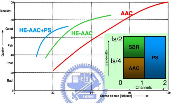
Figure 2: Quality comparison at different bit-rate among AAC, HE-AAC, and HE-AAC v.2 [6] ...2

Figure 3: Birdies effect occurring in LF of HE-AAC due to the insufficient bits...3

Figure 4: Enhanced Birdies effect by taking advantage of coupling coding 3 Figure 5: Basic architecture of HE-AAC encoder ...3

Figure 6: An example of reconstruction process of SBR ...5

Figure 7: Block diagram of HE-AAC encoder ...6

Figure 8: An example of the frequency table and time segment ...8

Figure 9: An example of VAR frame border to shift few sample points ...8

Figure 10: HF adjustment process of a noise-demand high resolution grid with three subbands b0,b1,b2...10

Figure 11: HF adjustment process of a noise-demand high resolution grid with three subbands b0,b1,b2...11

Figure 12: The syntax of the SBR extension data elements in coupling and non-coupling modes...13

Figure 13: Diagram of shared time segment in coupling and non-coupling modes ...14

Figure 14: An example of the optimal partition from i to j time unit with 3 time borders and 2 high resolution envelopes...16

Figure 15: Flowchart of the DP method proposed in [9] ...16

Figure 16: Decision flowchart of inverse filtering mode...20

Figure 17: The search range of quantized noise floor for different modes.22 Figure 18: Flowchart of the propose search method of the noise floor scale factor decision...23

Figure 19: The test track has high energy difference in high frequency...28

Figure 20: The high reconstruction error in weaker channel...28

Figure 21: The low reconstruction error in stronger channel ...28

Figure 22: The relationship between mean of relative error and Ψ whenΨis more than one in the right channel ...28

Figure 23: The relationship between mean of relative error and Ψ whenΨis less than one in the right channel ...29 Figure 24: The relationship between variance of relative error and Ψ

(8)

whenΨis more than one in the right channel ...29 Figure 25: The relationship between variance of relative error and Ψ

whenΨis less than one in the right channel ...29 Figure 26: The relationship between mean of relative error and Ψ

whenΨis more than one in the left channel ...30 Figure 27: The relationship between mean of relative error and Ψ

whenΨis less than one in the left channel ...30 Figure 28: The relationship between variance of relative error and Ψ

whenΨis more than one in the left channel ...30 Figure 29: The relationship between variance of relative error and Ψ

whenΨis less than one in the left channel ...31 Figure 30: Coupling Switch Flowchart...32 Figure 31: The variance in the ODGs of proposed coupling approaches at

80 kbps...35 Figure 32: The variance in the ODGs of proposed coupling approaches at

64 kbps...36 Figure 33: The variance in the ODGs of proposed coupling approaches at

48 kbps...37 Figure 34: The average ODGs of method M0 and M1 at 80kbps in 16

categories ...39 Figure 35: The average ODGs of method M0 and M1 at 64kbps in 16

categories ...39 Figure 36: The average ODGs of method M0 and M1 at 48kbps in 16

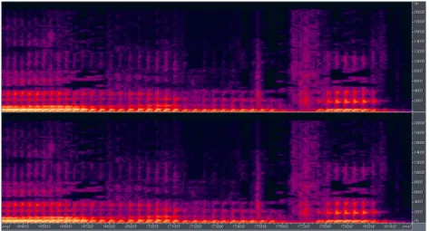
categories ...39 Figure 37: The suffered spectrum of the silence in the “impulse_m20_0db”

track...40 Figure 38: The spectrum of the “triangle1” track in the “TonalSignals” set

...40 Figure 39: Reconstructed spectrogram of the “triangle1” track in normal

mode...41 Figure 40: Reconstructed spectrogram of the “triangle1” track in coupling

mode...41 Figure 41: The result of the subjective test for coupling coding at 48kbps 42

(9)

Table List

Table 1: The parameter newBw decided by inverse filtering mode ...9 Table 2: The scenarios of the ten bit-consuming stage ...15 Table 3: Comparison of the grid criterion in the normal/coupling mode....18 Table 4: The twelve tracks recommended by MPEG...34 Table 5: Objective measurements through the ODGs for proposed coupling

approach at 80 kbps ...35 Table 6: Objective measurements through the ODGs for proposed coupling

approach at 64 kbps ...36 Table 7: Objective measurements through the ODGs for proposed coupling

approach at 48 kbps ...37 Table 8: The PSPLab audio database [13] ...38

(10)

Chapter 1 Introduction

MPEG-4 HE-AAC (High Efficiency Advanced Audio Coding) is the extension of the conventional AAC [1] by supporting the SBR (Spectral Band Replication) [2][3][4][5]. The basic principle of SBR is to reconstruct the high frequency spectral bands by replicating the low frequency spectral bands. The resulting codec is referred to as the MPEG-4 HE-AAC or AACplus. Besides taking the SBR as the bandwidth extension tool, the PS (parametric stereo) [6][7][8] coding is further incorporated as the channel reduction tool. The integrated codec is referred to MPEG-4 HE-AAC version 2. Figure 1 illustrates the scheme of HE-AAC and HE-AAC version 2.

AAC

SBR

PS

HE-AAC V1 HE-AAC V2

AAC

SBR

PS

HE-AAC V1 HE-AAC V2

Figure 1: Diagram of the HE-AAC and HE-AAC v.2 [9]

To fit a variety of situations of demand, the three coding schemes are applied to the different bit rates. In order to maintain the audio quality at low bit rate, HE-AAC is adapted among the 48 ~ 96 kbps. Furthermore, to satisfy the requirement of very low bit rate lower than 48 kbps, HE-AAC version 2 is proposed to overcome the challenge. Figure 2 illustrates the relationship between the bit rate and the perceptual quality. However, the efficiency of the complete system is determined largely by the cooperation of the three modules. Any unsuitable design of anyone of the three modules will affect the effect of the remainders, and hence destroy seriously the quality of the HE-AAC version 2.

This thesis will focus on the coupling coding in SBR. The principle of the coupling coding is to transform the left/right (L/R) energy signals into average/ratio (A/R) mode to eliminate signal correlation and take advantage of parameter sharing to

(11)

save bits. Especially, at very low bit rate, the bit shortage will result in many annoying artifacts at the low frequency in AAC. Hence, the purpose of coupling coding is to save the consuming bits of the high frequency to promote the low frequency quality. Figure 3 shows an example of a common artifact, known as “birdies effect” [10], at the low frequency part due to lack of bits in AAC. The spectral valley is visible in the low frequency spectrum encoded by AAC. Figure 4 shows the artifact is enhanced largely once AAC is supplied with enough bits.

0 32 64 96 128 0 20 40 60 80 100 Q ua lit y Excellent Poor Fair Good

Stereo bit-rate [kbit/sec] Bad HE-AAC+PS AAC HE-AAC B an dw id th Channels

0

2 fs/2

AAC

fs/4

AAC

SBR

AAC SBR PS

1

0 32 64 96 128 0 20 40 60 80 100 Q ua lit y Excellent Poor Fair Good

Stereo bit-rate [kbit/sec] Bad HE-AAC+PS HE-AAC+PS AAC HE-AAC B an dw id th Channels

0

2 fs/2

AAC

fs/4

AAC

SBR

fs/4

AAC

SBR

AAC

SBR

AAC SBR PS

1

Figure 2: Quality comparison at different bit-rate among AAC, HE-AAC, and

HE-AAC v.2 [6]

Figure 5 illustrates the block diagram of HE-AAC encoder. This thesis considers the coupling coding design through four design issues. The first and second issues are decision of shared T/F grid [9] parameter and shared inverse filtering intensity [11][12]. Furthermore, according to the constraint in the coupling mode, the difference values of quantized value of the specific parameters, named as noise floor scale factors [11][12], between two channels should be limited. Therefore, selecting suitable quantized noise floor scale factors for the two channels is the third issue. Finally, the last issue is coupling switch method which need to consider the tradeoff between high band quality and demand bits, and some possible risk of quality degradation.

(12)

Figure 3: Birdies effect occurring in LF of HE-AAC due to the insufficient bits

Figure 4: Enhanced Birdies effect by taking advantage of coupling coding

QMF

Analysis SynthesisQMF AAC CoreEncoder SBR

Encoder FormatterBitstream PCM

bitstream

Figure 5: Basic architecture of HE-AAC encoder

This thesis is organized as follow. Chapter 2 introduces the backgrounds on the fundamental knowledge of MPEG-4 HE-AAC. In Chapter 3, the five design issues of the coupling coding in MPEG-4 HE-AAC will be investigated, which include coupling switch method, decision of shared T/F grid parameter, decision of shared inverse filtering intensity, decision of the noise floor scalefactors. Chapter 4 conducts

(13)

experiment to verify performance of the proposed coupling coding method. Chapter 5 gives a conclusion on this thesis.

(14)

Chapter 2 Backgrounds

This chapter introduces some fundamental background of MPEG-4 HE-AAC. Especially, the three modules related to the coupling coding in SBR are also described.

2.1 MPEG-4

High Efficiency AAC

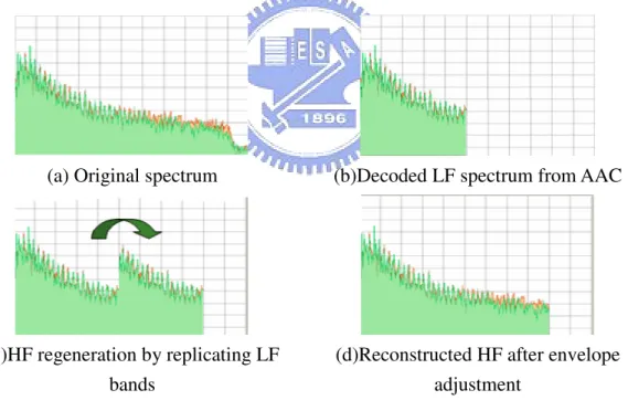
By the cooperation of both SBR and the conventional AAC, the HE-AAC can maintain the high audio quality at very low bit rate. The SBR takes care of the high frequency contents, and relatively the AAC encoder compresses the low frequency contents. Because of the few bits consuming of SBR, the most of available bits are supplied for AAC to maintain the quality of low frequency. Figure 6 illustrates the reconstruction process of SBR.

(a) Original spectrum (b)Decoded LF spectrum from AAC

(c)HF regeneration by replicating LF bands

(d)Reconstructed HF after envelope adjustment

Figure 6: An example of reconstruction process of SBR

The HE-AAC decoder reconstructs the high frequency by replicating the low frequency decoded from AAC, and then it will adjust the tonality of the replicated low band to be close to the tonality of the original high band by comparing the difference between the content of the high and low bands. Furthermore, there are two main modules in SBR encoder. One is the time/frequency grid module, and another is the high frequency adjustment module. In the time/frequency grid module, it splits the high bands into several T/F grids. Each T/F grid records the average energy to the

(15)

HE-AAC decoder. On the other hand, the HF adjustment module records the difference between the original and replicated contents of high frequency part. Besides the basic reconstruction operation, the data-rate reduction tool, Coupling coding, is adopted to further eliminate the signal correlation and save consuming bits of high frequency by domain transformation of envelope data and parameter sharing. The saved bits by the coupling coding mechanism can supply to AAC to promote low frequency quality effectively, and achieve the optimal overall quality.

! "" ! "" # $ # $ Input Signal Coded Audio Stream % % & & ! "" ! "" # $ # $_$ # # $_$ # # $ Input Signal Coded Audio Stream % % & &

(16)

2.2 Related Modules in SBR to Coupling Coding

In this section, three important modules related to coupling coding will be introduced. They include the time/frequency grid, the chirp factor used in the inverse filtering operation, and the tonality controlling factor Q. The understanding of the three issues will affect the design of the coupling coding largely.

2.2.1 Time/Frequency Grid in HE-AAC

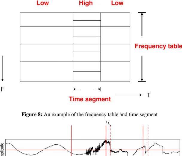
This subsection introduces the protocol about the time/frequency grid in HE-AAC. Adaptive time and frequency resolution are incorporated into SBR for the envelope coding and adjustment. The SBR replicates the low frequency signal to high frequency signal. The QMF subbands in SBR range will be segmented into several grids by divisions from the T/F dimension. The successive samples in QMF subbands are integrated into a “time envelope”. The successive subbands are segmented into several uniform or non-uniform bands with different bandwidth by choosing one of the frequency band tables. T/F grid which describes time segments and associated frequency tables is the basic reconstructed unit in the subsequent SBR coding process. The average energy in a grid will be used to get the rescale ratio, which is over the energy of the duplicated low bands. It implies that the locations of time borders and the resolution of the envelopes determine the accuracy of the replication and the audio quality. There are three components in the time/frequency grid module as follows

Frequency table Time segment Frame class

The frequency domain resolution is determining by choosing from the different frequency tables in the SBR. Frequency table affect the precision of tone addition and the low frequency which will be replicated for reconstruction high frequency in the decoder. There are five frequency tables in SBR. High resolution frequency band table and low resolution frequency band table are two available resolution tables that can be selected for every envelope of SBR frame. Noise floor frequency band table and limiter frequency band table correspond respectively to the noise floor and the limiter. All frequency band tables are derived from the master frequency band table. The master frequency tables are defined by functions and the arguments are transmitted in the SBR header. The time borders affect the resolution in the time domain. The time

(17)

borders are more flexible than frequency band table. It contains the number of envelopes in SBR frame and locations of time borders. There are 32 samples in the time domain of one SBR frame. But there are only 16 locations in the SBR frame for the time borders. Because of the constraint in SBR, there are 5 time borders if frame class is VARVAR. The other frame class only has 4 time borders at most.

There are four different SBR frame classes, FIXFIX, FIXVAR, VARFIX, and VARVAR in the SBR time/frequency grid. The four classes refer to whether locations of leading and trailing SBR frame boundaries are variable. HE-AAC allows the boundary between the two frames to shift few sample. It make time domain segment more flexible. Figure 9 is an example of the boundary shift few sample to match the signal.

T

F

Time segment

High

Low

Frequency table

Figure 8: An example of the frequency table and time segment

(18)

2.2.2 Chirp Factor of Inverse Filtering

The high bands in SBR decoder are reconstructed from the low bands. Hence, if the tonality of the replicated low bands will not match the features of the original high bands, the inverse filtering is applied to eliminate the excess tone component of the replicated low bands. The inverse filtering process is performed in the two steps. First, the linear prediction is applied on the replicated low bands. Then the actual inverse filtering is performed respectively for each of the replicated low bands patched to the high bands. The resultant high band generated in SBR decoder is obtained as

{

( , 1) ( , 2)

}

) , ( ) , ( 1 2 0 ⋅ − + ⋅ ⋅ − ⋅ − =X p l a X p l a X p l l k

XHigh Low α Low α Low , (1)

where α is the chirp factor that can control the inverse filtering level, XLow is the low band signal analyzed from the output of AAC decoder, and a0,a1 are the prediction coefficients which are used to filter the subband signal in the inverse filtering .The chirp factor can remove the location of the poles of the inverse filter and affect the degree of the harmonic attenuation in the high frequency generator. According to the standard [2] , the calculation of the chirp factor is defined as

( )

_{( )}

( )

_{( )}

,0 i NQ 0.015625 0.015625 0 < ≤ ≥ < = i tempBw f i tempBw i tempBw if i α , (2)

where N_Q is number of noise floor bands, and tempBw

( )

i is calculated as

( )

_{( )}

( )

_{( )}

i NQ i if i newBw i if i newBw i tempBw ≤ < ≥ ⋅ + ⋅ < ⋅ + ⋅ = ,0 newBw 09375 . 0 90625 . 0 newBw 25 . 0 75 . 0 ' ' ' ' α α α α _, (3) where _{α is the α values calculated in the previous SBR frame, and}' _newBw_is decided by inverse filtering mode of current frame and previous frame according to Table 1.

Table 1: The parameter newBw decided by inverse filtering mode

bs_invf_mode(i)

bs_invf_mode(i)´ Off Low Intermediate Strong

Off 0.0 0.6 0.9 0.98

Low 0.6 0.75 0.9 0.98

Intermediate 0.0 0.75 0.9 0.98

Strong 0.0 0.75 0.9 0.98

2.2.3 Noise Floor Scale Factor Q

(19)

adjustment of the each subband in the high resolution grid and the tone-noise additive level. There are two different types of the envelope scaling for the noise-demand and the tone-demand grid according to their requirement of content. In the noise-demand grid, the magnitudes of the replicated bands are adjusted by a gain control factor defined as [11] k r k o k ND k _E _Q E G + ⋅ = 1 1 _, (4) where o k E and r k

E are the average energy of the original high frequency signal and the replicated low frequency signal respectively in the kth high resolution grid, and

k

Q is the noise floor scale factor. After the envelope scaling, the random noise is

added to the high frequency with level defined as

k k o k n k _Q Q E C + ⋅ = 1 . (5)

Similarly, the gain control factor in the tone-demand grid is defined as

k k r k o k TD k _Q Q E E G + ⋅ = 1 . (6)

Also, the energy amount for the compensated tone is defined as

k o k t k E _Q C + ⋅ = 1 1 _. (7) Figure 10 and Figure 11 illustrate the two different adjustment results for the noise- and tone- demand grids.

( )

ND 2 k r k G E ⋅

( )

ND 2 k r k G E ⋅

( )

ND 2 k r k G E ⋅ n k C n k C n k C 0 b b1 b2

( )

ND 2 k r k G E ⋅

( )

ND 2 k r k G E ⋅

( )

ND 2 k r k G E ⋅ n k C n k C n k C

( )

ND 2 k r k G E ⋅

( )

ND 2 k r k G E ⋅

( )

ND 2 k r k G E ⋅ n k C n k C n k C 0 b b1 b2 Noise-demand grid scaling compensation

( )

ND 2 k r k G E ⋅

( )

ND 2 k r k G E ⋅

( )

ND 2 k r k G E ⋅ n k C n k C n k C 0 b b1 b2

( )

ND 2 k r k G E ⋅

( )

ND 2 k r k G E ⋅

( )

ND 2 k r k G E ⋅ n k C n k C n k C

( )

ND 2 k r k G E ⋅

( )

ND 2 k r k G E ⋅

( )

ND 2 k r k G E ⋅ n k C n k C n k C 0 b b1 b2 Noise-demand grid scaling compensation

Figure 10: HF adjustment process of a noise-demand high resolution grid with three

(20)

( )

TD 2 k r k G E ⋅

( )

TD 2 k r k G E ⋅

( )

TD 2 k r k G E ⋅ n k C t k C n k C 0 b b1 b2

( )

TD 2 k r k G E ⋅

( )

TD 2 k r k G E ⋅

( )

TD 2 k r k G E ⋅ n k C t k C n k C 0 b b1 b2 Tone-demand grid scaling compensation

( )

TD 2 k r k G E ⋅

( )

TD 2 k r k G E ⋅

( )

TD 2 k r k G E ⋅ n k C t k C n k C 0 b b1 b2

( )

TD 2 k r k G E ⋅

( )

TD 2 k r k G E ⋅

( )

TD 2 k r k G E ⋅ n k C t k C n k C 0 b b1 b2 Tone-demand grid scaling compensation

Figure 11: HF adjustment process of a noise-demand high resolution grid with three

(21)

Chapter 3 Design of Coupling

Coding in SBR

As the fundamentals of the coupling coding design, this chapter reviews firstly the coupling coding schemes defined in the HE-AAC standard [2]. Furthermore, based on our related work [9][11] about the designs of the T/F grid and tonality compensation, the thesis extends the works into the coupling coding method. The extension should consider the risk of parameter sharing. For example, the T/F grid sharing will result in the coarse reconstructed envelope or the more bits consuming. Also, the sharing of the chirp factor and noise-floor factor may destroy the tonality accuracy of some channel and lead to the quality degradation. Finally, the huge ratio of the left and right energy channels will result in the data correlation reduction and the large quantization error. A coupling switching method considering the abnormal phenomenon is proposed to compromise the tradeoff between the quality and the bits reduction.

3.1 Overview of Coupling Coding Schemes in HE-AAC

For the energy data of the spectral envelop extracted from time/frequency (T/F) grids, there are several processes, including quantization operation, the DPCM and the Huffman entropy coding, to be applied to reduce the data rate in turn. Furthermore, to reduce the data redundancy of the stereo energy channels, the coupling mode is adapted to transform the Left/Right (L/R) energy channels into Average/Ratio (A/R) mode to eliminate signal correlation. To meet the inherent requirement of the coupling, the parameters for T/F grid and inverse filtering need to be shared by A/R channels in coupling mode. Figure 12 illustrates the syntax of the SBR extension data elements in the two modes. It shows that both the T/F grid and the controlling parameter of inverse filtering level, that is chirp factor, should be shared.

In summary, there are five critical points when the coupling mode is switched on. The five terms are as follows:

Transform L/R mode into A/R mode Share Time/Frequency grid

Share chirp factor of inverse filtering

(22)

The difference of quantized noise-floor scalefactors between the two

channels is restricting to the range from 0 to 12 by the syntax constraint.

' & ()* (+* ()* (+* ()* (+* , , ' & ()* (+* ()* (+* ()* (+* , , ' & ()* (+* , , ' & ()* (+* , , ! - " . & # &

Figure 12: The syntax of the SBR extension data elements in coupling and

non-coupling modes

3.2 Decision of Shared T/F Grid

Instead of using the individual set of time segments as the normal L/R mode, there can be only a common segment set in the coupling mode. Although the sharing of side information can save bits, the quality artifact may occur due to inaccurate segment. Hence, the quality degradation should be considered. For the optimal time segments of the signal subbands of the L/R channels in the normal mode, a decision method based on dynamic programming approach has been proposed in our other work [9]. In this section, the modified decision method for coupling mode is proposed to determine the optimal common segment set and measure the affect for quality.

(23)

( ) ( ) = ∗ L L G L Arg MinOG G ( ) ( ) = ∗ R R G R Arg MinOG G ( ) ( ) = ∗ C C G C Arg MinOG G ( ) ( ) = ∗ L L G L Arg MinOG G ( ) ( ) = ∗ R R G R Arg MinOG G ( ) ( ) = ∗ C C G C Arg MinOG G

Figure 13: Diagram of shared time segment in coupling and non-coupling modes 3.2.1 Design of T/F Grid by Dynamic Programming in Non-coupling Mode

In [9], a decision method of T/F grid by the dynamic programming (DP) in non-coupling mode has been proposed. The basic concept of the DP method is to search the optimal grid in the all possible grids in individual channel by an efficient

recursive procedure. The resultant grid _G∗_{searched by the method will be an}

optimal solution to make the average of the energy difference (reconstructed energy error) to the original signal energy ratios (DSR) in all quality measurement units, named critical units, minimum. That is,

( )

(

)

(

MinDSR G

)

Arg G G = ∗ _, (8) where DSR

( )

G is defined as

( )

_{( )}

c DSR G DSR cG c # ∈ = , (9)

where c is the critical unit, #

( )

c means the number of critical units, and DSRc is

the reconstruction error of the critical unit c in the frame. The lengths of the critical unit are defined as four sample points and the critical band bandwidth for time and frequency direction respectively in [9].

The number of the time borders and the associated frequency resolution determine the total number of the girds and also affects the resultant DSR. The dynamic programming for DSR analysis is shown as

(24)

{

}

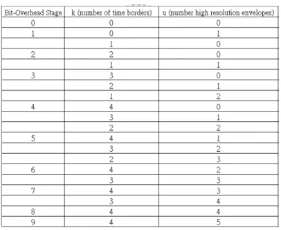
1 k u 0 , 4 k 0 ; 8 j i 0 , 1, 1 2 , 2 1 , 0 2 , 2 , 1 2 , 2 0 , 0 2 , 2 1 1 , 2 , 2 + ≤ ≤ ≤ ≤ ≤ < ≤ + + = − − − − ≤ ≤ + u k j t t i u k j t t i j t i u k j i Min DSR DSR DSR DSR DSR (10)

where i, j are the border of the time slot consisting of two samples, k is the number of the time borders, and u is the number of the high resolution envelopes. The

notation ku

j i D ,

, means the optimal DSR from i to j with k time borders and u high

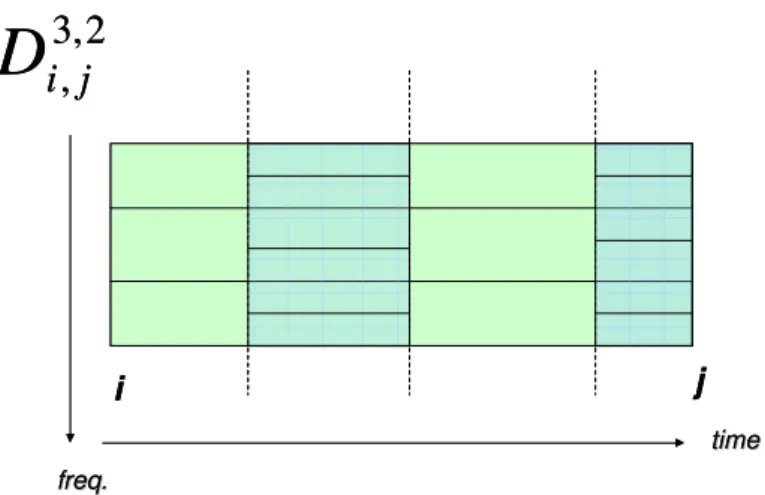
resolution envelope. According to [9], there are ten different bit-consuming stages defined in the dynamic programming method. Each stage indicates the different number of time borders and high resolution envelopes in one SBR frame. The scenarios of the ten stages are described in Table 2. Figure 14 illustrates the optimal partition from i to j with 3 time borders and 2 high resolution envelopes.

(25)

i j

2 ,

3 , j

i

D

time time freq. freq. i j

2 ,

3 , j

i

D

time time freq. freq.

Figure 14: An example of the optimal partition from i to j time unit with 3 time

borders and 2 high resolution envelopes

Figure 15 is the flowchart of the dynamic programming method for searching optimal T/F grid. The loop will consider all passable resolution grids. In the loop, it will have an objective function for determining the optimal T/F grid in the same bit-consuming stage. There is another efficiency checking for switching different stages. The dynamic programming method searches the optimal grid from the lower bit-consuming stages to the higher bit-consuming stages. Because the different bit-consuming stages have different requirement of bits, the grid decision in the different stages must consider the tradeoff of bits and quality.

Stage > 9 Stage > 9 Check efficiency Check efficiency Increase Stage Increase Stage

Record efficient grid

Record efficient grid No

Yes

No

Find optimal T/F grid

End End Begin Begin Stage > 9 Stage > 9 Check efficiency Check efficiency Increase Stage Increase Stage

Record efficient grid

Record efficient grid No

Yes

No

Find optimal T/F grid

End

Begin

(26)

3.2.2 Design of T/F Grid by Dynamic Programming in Coupling Mode

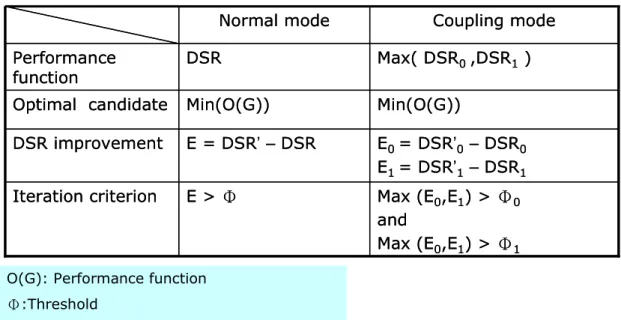
Because of the sharing of the T/F grid, the two criterions used in the above DP method must be modified to simultaneously consider the content of two channels in the coupling mode. There is an objective function which measures the grids in the DP search method. In the normal mode, the objective function is defined as the DSR value described above. To consider both the two DSR values from L/R channels in the coupling mode, the objective function is modified as

(

0, 1

)

(G Max DSR DSR

O = , (11)

where DSR0 and DSR1 are the DSR values of left and right channel respectively. To

ensure the quality of worst channel, the conservative choice of the resultant grid is adopted in the criterion. The optimal grid is the minimum solution of the objective function (11).

On the other hand, the iteration criterion of the DP method in the normal mode involves the improvement of DSR in the current resolution. If the improvement of DSR is over the threshold depending on the bit rate, it will update the higher resolution T/F grid to improve the quality. The improvement is defined as

DSR DSR

E= '− _, ₍₁₂₎

where _DSR'_{is the optimal DSR for the preceding bit-consuming stage. Similarly, in}

the coupling mode, there are two improvements of DSR which are defined as

1 ' 1 1 0 ' 0 0 DSR DSR E DSR DSR E − = − = . (13)

The modified iteration criterion is to satisfied the two conditions as follows

(

0 1

)

1 max =max E ,E >Φ E , (14)

(

0 1

)

2 min =min E ,E >Φ E , (15)

where Φ1 and Φ2 are the threshold of iteration criterion. The modification of the

iteration criterion can ensure that the improvement of both the DSR values of the two channels are over a low bound, and at least one of the DSR improvements can exceed the large degree to show the efficiency of the new stage.

(27)

Table 3: Comparison of the grid criterion in the normal/coupling mode ’ – ’ – ’ – ! ! " # ! " " $ % ## & % ' # ( % # ’ – ’ – ’ – ! ! " # ! " " $ % ## & % ' # ( % # ) *) %# + % # ' * %

3.3 Decision of Shared Inverse Filtering Intensity

In SBR, the inverse filtering is adopted to eliminate excess tones in low bands to fit the tonality of high bands. The different chirp factors, which are the parameter to control the intensity level of the inverse filtering, are assigned to L/R channels in the normal mode. Similarly, according to the regulation of the standard [2], only single chirp factor can be used in the coupling mode. Once the difference of the tonality contents is dominate, the possible artifact suffering from the unsuitable inverse filtering under the constraint is able to be anticipated. Hence, the risk of the inverse filtering with the same intensity level for the stereo channels in the coupling mode should be considered.

3.3.1 Decision of Inverse Filtering Intensity in Non-coupling Mode

In [11][12] of our another work, a compensation method of additional tone and noise to maintain the dB-difference of the tone and noise component has been proposed. In the non-coupling mode, based on the method, the selecting method of inverse filtering level is depended on the tonality between the high bands and the low bands. According to the syntax, each specific “noise band” has an inverse filtering mode individually. Furthermore, a noise band may include several high-resolution grids. Therefore, the tonality of the noise band is defined in [11][12] as

(28)

∈ = ∆ i NB N T i i NB max | , (16)

where Ti is the energy of tone in the ith high resolution grid of the noise band, Ni is the

energy of noise floor in the ith high resolution grid of noise band, and NB is the noise

bands in the SBR frame. From (16), the maximum tonality among the high resolution grids stands for the tonality of the noise band. The goal of the inverse filtering mode is to imply that the tonality of the replicated low frequency band can approach the tonality of the original high frequency band, that is

h NG l NG =∆ ∆ˆ , (17) where l NG

∆ˆ is the tonality of the replicated low frequency band, h NG

∆ is the tonality

of the original high frequency band. The optimal chirp factor can be evaluated from

h h l l N T N T = − ) 1 ( _α2 , ₍₁₈₎

where α is chirp factor. Then the practice chirp factor can be searched in the Table 1

to approximate the optimal one.

3.3.2 Decision of Inverse Filtering Intensity in Coupling Mode

However, in the coupling mode, there is only one inverse filtering mode for two channels. To measure the influence to the resultant tonalities, the distortion function of the shared chirp factor is defined as

( )

₀ ₀ 2 ₁ ₁ 2 h l h l x x x f = ∆ −∆ + ∆ −∆ , (19) where _x₌₁₋_α2_, 0 l ∆ , 1 l

∆ are the tonality of low frequency in the left and right

channel respectively, and 0

h

∆ , 1

h

∆ are the tonality of high frequency in the left and

right channel respectively. Hence, the optimal chirp factor shared by the two channels in the coupling mode should be the minimum solution of the distortion function (19). The optimal solution can be calculated by solving the equation of the one order differential of the distortion function,

(

)

2

(

)

0 2_∆0 _∆0₋_∆0 ₊ _∆1 _∆1 ₋_∆1 ₌ h l l h l l x x . (20)

Form (20), the optimal chirp factor in the coupling mode can be evaluated from

( ) ( )

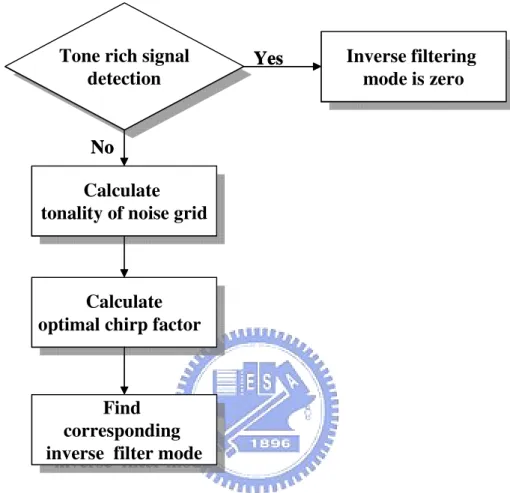
₀ 2 ₁ 2 1 1 0 0 2 1 l l h l h l x ∆ + ∆ ∆ ∆ + ∆ ∆ = − = α . ₍₂₁₎

(29)

mechanism must be turned off for the tone-rich frame, because the tone-rich signal must not be processed in order to maintain the structure completeness of the tone rich signal. Figure 16 illustrates the inverse filtering mode decision in the coupling mode.

Calculate tonality of noise grid

Inverse filtering mode is zero

Calculate optimal chirp factor

Tone rich signal detection

Tone rich signal

detection Yes No

Find corresponding inverse filter mode

Calculate tonality of noise grid

Inverse filtering mode is zero

Calculate optimal chirp factor

Tone rich signal detection

Tone rich signal

detection Yes No

Find corresponding inverse filter mode

Figure 16: Decision flowchart of inverse filtering mode

3.4 Decision of Noise Floor Scalefactor

As the quantization value of the noise floor factor Q, the quantized noise floor scale factor q is the parameter adjusting the reconstructed tone-noise content. However, according to the syntax constraint, in the coupling mode, the difference of q values between the two channels can not be larger than twelve. Because of the restriction, the optimal q values in the coupling mode may be different from the ones in the normal mode. In this section, the modified decision method for coupling mode is proposed to determine the optimal quantized noise floor scale factor.

In [11][12] of our another work, the proposed method in the normal mode can decide the optimal q to maintain the minimum distortion of the dB-differences among all the high resolution grids contained in the single noise grid. There is only one q

(30)

value shared in a single noise grid which includes several high resolution grids. The distortion function is defined as

( )

(

( )

)

(

( )

)

∈ ∈ ∆ − ∆ + ∆ − ∆ = TD k k TD k ND k k ND k Q Q Q D 2 2, ₍₂₂₎

where ∆k is the ideal tone/noise dB-difference of original signal in

th k high resolution grid, ND k ∆ , TD k

∆ are the resultant tone/noise dB-difference by q, if _kth_high

resolution grid is noise demand grid and tone demand grid respectively. Hence, the optimal q value must be chosen to minimize the distortion function.

( )

[

]

{

DQ

}

Arg Q Q min * ₌ (23) In the coupling mode, for the quantization process of the noise floor factor Q values, the Q values should be firstly changed into A/R mode from the L/R mode to eliminate signal correlation. As mentioned above, in the coupling mode, the ratio channel of the quantized noise floor needs to be restricted as

[ ]

0,24

∈

ratio

q . (24)

And, the quantization formula of qratio is defined as

( )

_{( )}

0.5 12 , , log , = 2 + + l k Q l k Q INT l k q right left ratio , (25)

where Qleft and Qright are the noise floor of left and right channel respectively, k is

the index of the frequency table band in SBR, l is the index of the envelope. On the other hand, the dequantization formula of the q value in the L/R mod is defined as

q

Q₌₂6− _. ₍₂₆₎

By substituting (26) into (25), it results in

12 2 2 log2 6₆_-_q_R + ≈ −qL ratio q , (27)

where qLand qR are the quantized noise scale factor in left and right channel

respectively. Hence, from (24) and (27), the constraint of the noise floor scale factor pair of the L/R mode is derived as

[

−12,12

]

∈

− L R q

q . (28)

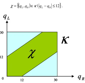
Hence, the search range of the candidates of quantized L/R noise scale factor pair in the coupling mode is smaller than the range in the normal mode. As shown in Figure

17, range Κ is the search scope in the normal mode, the contracted rangeχ is the

search scope in the coupling mode, where

(

)

{

, _∈ 2|0_≤ , _≤30

}

= q_L q_R Z q_L q_R

(31)

(

)

{

, ∈ | − ≤12

}

= q_L q_R κ q_L q_R χ . (30) 0 ₁₂ 12 30 30 R

q

L

q

χ

κ

0 ₁₂ 12 30 30 R

q

L

q

χ

0 ₁₂ 12 30 30 R

q

L

q

0 ₁₂ 12 30 30 R

q

L

q

χ

κ

Figure 17: The search range of quantized noise floor for different modes

Hence, the distortion measure function needs to be modified in the coupling mode to consider the two channel distortion under the inherent constraint. As an extension of (22), the modified distortion function for the coupling mode is defined as

(

_L, _R

)

=

(

_L

( )

_L

)

+

(

_R

( )

_R

) (

, _L, _R

)

∈χ

C q q DQ q DQ q q q

D (31)

where Q

( )

q is the de-quantization function of q. Furthermore, the optimal (QL,QR)

should be decided by choosing the minimum solution pair (qL, qR) for the distortion

function, that is

(

)

{

₍ ₎

[

C

(

L R

)

]

}

R q L q R L q Arg D q q q , min , , * * χ ∈ = . ₍₃₂₎

Different from the brute-force method to search optimal solution, a modified search method is proposed to reduce the time cost. Figure 18 illustrates the proposed noise floor scale factor decision. We expected that the most pairs of the optimal quantized noise floor scale factor for each individual channel can conform to the constraint of coupling mode. It means the first searching target should be the ones. Once the special pair can fit the constraint, the final optimal solution is also found and the search procedure can be stopped. In summary, we search the optimal scale factors for each channel after the distortion calculation and check of the difference between two channels. If the optimal scale factors for each individual channel can’t conform to the constraint, it will search the remained candidate pairs for the optimal solution of the coupling distortion function.

(32)

Find

Min_q

_L

, Min_q

_R

Find

Min_q

_L

, Min_q

_R

|Min_q

_L

-Min_q

_R

|>12

|Min_q

_L

-Min_q

_R

|>12

Find (q

_R

,q

_L

)

minimum D

_C

(q

_R

,q

_L

)

Find (q

_R

,q

_L

)

minimum D

_C

(q

_R

,q

∈

_L

χ

)

q

_L

=Min_q

_L

q

_R

=Min_q

_R

q

_L

=Min_q

_L

q

_R

=Min_q

_R

Yes

No

Calculate D(q)

for all q values

Calculate D(q)

for all q values

Find

Min_q

_L

, Min_q

_R

Find

Min_q

_L

, Min_q

_R

|Min_q

_L

-Min_q

_R

|>12

|Min_q

_L

-Min_q

_R

|>12

Find (q

_R

,q

_L

)

minimum D

_C

(q

_R

,q

_L

)

Find (q

_R

,q

_L

)

minimum D

_C

(q

_R

,q

_L

χ

)

∈

Find (q

_R

,q

_L

)

minimum D

_C

(q

_R

,q

_L

)

Find (q

_R

,q

_L

)

minimum D

_C

(q

_R

,q

_L

χ

)

∈

q

_L

=Min_q

_L

q

_R

=Min_q

_R

q

_L

=Min_q

_L

q

_R

=Min_q

_R

Yes

No

Calculate D(q)

for all q values

Calculate D(q)

for all q values

Figure 18: Flowchart of the propose search method of the noise floor scale factor

decision

3.5 Coupling Switch Method

The human hearing is relatively more sensitive for the low frequency then the high frequency. To improve the quality of the LF component, the basic objective of the coupling is to save the consuming bits of the HF part as many as possible under the constraint of the least quality requirement. Unlike the aspects of the intensity coding or M/S coding, the main risk of the coupling coding is from the more inaccurate envelope of reconstructed high bands, not fine structure loosing. Because the robustness of SBR, in general, the coupling coding can save a large amount of consuming bits, and promote overall quality under very small risks. However, from

(33)

both the two aspects, including the data correlation degree and quantization error variation, the huge difference of the left and right energy channels may result in the degradation of the coding gain and the increase of the reconstruction error. Based on the two points, a coupling switch decision method is proposed for the tradeoff between HF quality and demand bits. Taking into account the above risks with the least bits consuming, the optimal represent domain of the signal, either L/R or A/R mode, will be chosen.

3.5.1 Quantization error analysis

As the following, the variations of the quantization errors at different mode will be analyzed. The spectral energy is quantized into the scale factor by taking time-frequency grid of the current frame as the recorder units. There are different quantization methods in the normal mode and the coupling mode. The quantization formula in the normal mode is defined as

( )

E Q l L l k E a INT l k E = ⋅ ,0 +0.5 ,0≤ ≤ 64 , log max , 2 , (33) where = = = 1 _ _ , 1 0 _ _ , 2 res amp bs if res amp bs if

a , k is the index of the frequency table band in SBR,

l is the index of the envelope, LE is the number of envelope in current SBR frame, and

E(k,l) means the energy of input signal in the normal mode, and also means the

average energy between the stereo channel in coupling mode. Furthermore, the right channel quantization formula in the coupling mode is defined as

( )

k l INT

(

a

(

E

( )

k l

)

panOffset

(

bs amp res

)

E_QRight , = ⋅log₂ , +0.5 + _ _ , ₍₃₄₎

where E(k,l) is the energy ratio between the stereo channel. On the other hand, the de-quantization method for the normal mode in HE-AAC decoder is defined as

( )

= ⋅ ( ) _≤≤_<<

_{( )}

l r n k L l l k E E_akl E Orig ₀ 0 , 2 64 , , , (35)

where E(k,l) is decoded envelope scale factor. Also, by the incorporation of the de-A/R operation, the de-quantization method in the coupling mode is defined as

( )

( ) ( ) ( ) _≤ _<

( )

< ≤ + ⋅ = ₋ + l r n k L l l k E E a l k E res amp bs panOffset a l k E LeftQrig 0 0 , 2 1 2 64 , _{_} _{_} _, 1 , 1 0 , (36)

(34)

( )

( ) ( ) ( ) _≤ _<

( )

< ≤ + ⋅ = ₋ + l r n k L l l k E E a res amp bs panOffset l k E a l k E RightQrig 0 0 , 2 1 2 64 , _, _{_} _{_} 1 , 1 0 , (37)

where E0,E1 represent the decoded A/R envelope scale factors.

Through the quantization formulas above, the reconstruction error can be estimated. From (33) and (35), the reconstruction value in the normal mode can be calculated as a E a E ) 5 . 0 ) 0 ), 64 ( max(log int( ' 2 2 64 + × × = , (38)

where E is the energy of original signal. From (38), If E is smaller than 64, _{E is}'

always 64. If E is greater than 64, _{E is calculated as}'

a E a E ) 5 . 0 ) 64 ( log int( ' 2 2 64 + × × = . (39)

Form (39) , the relative error in the normal mode can be evaluated from

a E E E ε 2 1 ' − = − , (40)

where someεlocates at the range from -0.5 to 0.5. If ε is zero value, it implies there

is no reconstruction error.

From (33), (34), (36), and (37), the reconstruction value of two channels in the coupling mode is derived as

+ ⋅ ⋅ ⋅ = − + × − + + × 1 ) 5 . 0 ) ( log int( ) 5 . 0 ) 128 ( log int( ' 2 2 2 1 2 2 64 a E E a a E E a L R L R L E , (41) + ⋅ ⋅ × = − + × + + × 1 ) 5 . 0 ) ( log int( ) 5 . 0 ) 128 ( log int( ' 2 2 2 1 2 2 64 a E E a a E E a R R L R L E , (42)

where EL and ER are the energy of original signal. The ratio of the reconstructed and

original energies in the coupling mode can be evaluated from (41), (42), that is

1 2 2 2 2 2 1 2 1 ' + ⋅ Ψ + ⋅ Ψ = + + a a a L L E E ε ε ε ε ε , (43) a a a R R E E 2 1 1 ' 2 1 2 2 ε ε ε ⋅ Ψ + + ⋅ Ψ = , (44)

(35)

where R L E E =

Ψ , ε₁∈[−0.5,0.5] , and ε2∈[−1.5 ,0.5] . The constant ε1 is the

quantization error of the energy quantization process, and the constant ε2 is the

reconstruction error which results from the quantization process and the DPCM operation in the SBR.

3.5.2 Energy Abnormal Phenomenon

From (43) and (44), if Ψ is huge, the reconstruction error will approximate the

limit value as follows

a L L E E' 1 2 lim ε = ∞ → Ψ , (45) a R R E E' 1 2 2 lim ε ε− ∞ → Ψ = . (46)

On the other hand, if Ψ is very small, the reconstruction error will approximate the

limit value as follows

a L L E E 1 2 2 lim ' 0 ε ε+ → Ψ = , (47) a R R E E 1 2 lim ' 0 ε = → Ψ . (48) If the values R R E E' , L L E E'

are more close to one, it means the relative error is more

close to zero. However, from (40), (46), and (47), the two value ε1−ε2 andε1+ε2

occurring in the coupling mode may be much larger than the valueε in the normal

mode. This is because that the ε belongs the range from 0.5 to -0.5, and the

distribution of ε1−ε2 and ε1+ε2 is larger, that is ε1−ε2∈

[

−1 ,2

]

, and

[

2 ,1

]

2 1+ε ∈ −

ε . It implies that the reconstructed error of weaker channel may

abnormally become very large when the energy difference between the two channels is large. For example, Figure 19 is the spectrum of the test stereo signal to illustrate the error augment phenomenon. The test track has high energy difference in HF between L/R channels. As shown in Figure 20, it is the comparison of reconstruction signal between coupling and normal mode. The energy difference is about 3 dB between the reconstruction signals in the coupling and normal mode. Figure 21 indicates that the stronger channel has the nearer reconstruction signal between coupling and normal mode.

(36)

In order to limit the reconstruction error to the endurable range, it needs to find

the reasonable relative range of Ψ to switch coupling mode. Figure 22 and Figure

23 illustrate the relationship between Ψ and the mean of relative error in the right

channel. The mean of relative error is calculated as follows

2 5 . 0 5 . 0 1 5 . 1 2 1 1 1 2 1 2 2 1 5 . 2 1 ) ( ε ε ε ε ε d d mean a a a − − ⋅ Ψ + ⋅ Ψ + − = Ψ . (49)

The mean of relative error is close rapidly to the upper bound when Ψ is over 8, and

the coupling mechanism should be turned off to avoid the annoying phenomenon of

the error augment.Figure 24 and Figure 25 indicate the relationship between Ψ and

the variance of relative error in the right channel. The variance of relative error is calculated as follows

( )

1 2 5 . 0 5 . 0 1 5 . 1 2 2 1 1 2 1 2 2 1 5 . 2 1 ) ( var ε ε ε ε ε d d mean iance a a a − − − Ψ ⋅ Ψ + ⋅ Ψ + − = Ψ . (50)

The variance of relative error is also close rapidly to the upper bound when Ψ is

over 8. There is a trade-off between the reconstruction error and the saved bit, and hence a switch threshold is required to avoid extreme reconstruction error. Similarly,

Figure 26 and Figure 27 illustrate the relationship between Ψ and the mean of

relative error in the left channel. Figure 28 and Figure 29 indicate the relationship

between Ψ and the variance of relative error in the left channel. The mean and

variance of relative error is calculated as

2 1 5 . 0 5 . 0 1 5 . 1 2 1 1 2 2 2 1 5 . 2 1 ) ( ε ε ε ε ε d d mean a a a − − − + Ψ ⋅ Ψ + − = Ψ (51) and

( )

1 2 5 . 0 5 . 0 1 5 . 1 2 2 1 1 2 2 2 1 5 . 2 1 ) ( var ε ε ε ε ε d d mean iance a a a − − − − Ψ + Ψ ⋅ Ψ + − = Ψ (52)

for left channel, respectively. According to the mean and variance of relative error, the switch threshold is set to 8 to avoid the high relative error.

(37)

Figure 19: The test track has high energy difference in high frequency

Figure 20: The high reconstruction error in weaker channel

Figure 21: The low reconstruction error in stronger channel

(38)

than one in the right channel

Figure 23: The relationship between mean of relative error and Ψ whenΨis less than one in the right channel

Figure 24: The relationship between variance of relative error and Ψ whenΨis more than one in the right channel

Figure 25: The relationship between variance of relative error and Ψ whenΨis less than one in the right channel

(39)

Figure 26: The relationship between mean of relative error and Ψ whenΨis more than one in the left channel

Figure 27: The relationship between mean of relative error and Ψ whenΨis less than one in the left channel

Figure 28: The relationship between variance of relative error and Ψ whenΨis more than one in the left channel

(40)

Figure 29: The relationship between variance of relative error and Ψ whenΨis less than one in the left channel

3.5.3 Summary

Therefore, the criterion of the proposed coupling switch method focuses on the average energy difference in the SBR range to avoid the abnormal phenomenon. The average energy difference is calculated from the energy ratio which is divided by critical unit. The number of samples of critical band in high frequency is different from the number in the low frequency, hence the energy ratio must be normalized as follows,

( )

∈ ∈ − = F c c j r c j l c j Diff _c E E E , 2 , 2 log log , ₍₅₃₎

where c is the critical unit we used in Section 3.2, ci

j

E , _{is the j}th_{sample energy of}

critical unit c of channel i, and |c| is the number of samples of critical unit. Figure 30 illustrates the proposed coupling switch method which detects of the huge average energy difference.

(41)

Calculate average energy difference Calculate average energy difference Average energy difference > Threshold Average energy difference

> Threshold Use coupling modeUse coupling mode

Use normal mode

No Yes Calculate average energy difference Calculate average energy difference Average energy difference > Threshold Average energy difference

> Threshold Use coupling modeUse coupling mode

Use normal mode

No

Yes

(42)

Chapter 4 Experiments

In this chapter, the quality measurement is conducted on the NCTU_HEAAC platform. Extensive experiments are performed to prove the enhancement of the proposed methods on the MPEG test tracks and the music database [13] collected in PSPLAB.

4.1 Experiment Environment

Objective Quality Measurement Tool:

The tool called “EAQUAL” [14] is chosen to measure the audio quality in the objective test. EAQUAL stands for “Evaluation of Audio Quality”. The purpose of EAQUAL is to supply the audio objective quality measurement for coded/decoded audio signals especially useful for audio codec development. The implementation of EAQUAL is based on the ITU-R recommendation BS.1387 [15].

Subjective Quality Measurement Tool:

In subjective quality test, we use MUSHRA [16] to assist the assessment. Multi stimulus test with hidden anchors and reference has been designed to give a reliable and repeatable measure of the audio quality of intermediate-quality signals. MUSHRA has the advantage that it provides an absolute measure of the audio quality of the codec which can be compared directly with the reference. MUSHRA follows the test method and impairment scale recommended by the ITU-R BS.1116 [17].

(43)

4.2 Objective Quality Measurement in MPEG Test Tracks

MPEG twelve tracks include critical music balancing on the percussion, string, wind instruments, and human vocal. The features of these twelve tracks are shown in the Table 4. In this section, it will verify the quality enhancement of proposed methods in different bit rates based on the MPEG test tracks.

Table 4: The twelve tracks recommended by MPEG Signal Description

Tracks

Signals Mode Time (sec) Remark

1 es01 Vocal (Suzan Vega) stereo 10 (c)

2 es02 German speech stereo 8 (c)

3 es03 English speech stereo 7 (c)

4 sc01 Trumpet solo and orchestra stereo 10 (b) (d)

5 sc02 Orchestral piece stereo 12 (d)

6 sc03 Contemporary pop music stereo 11 (d)

7 si01 Harpsichord stereo 7 (b)

8 si02 Castanets stereo 7 (a)

9 si03 pitch pipe stereo 27 (b)

10 sm01 Bagpipes stereo 11 (b)

11 sm02 Glockenspiel stereo 10 (a) (b)

12 sm03 Plucked strings stereo 13 (a) (b)

Remarks:

(a) Transients: pre-echo sensitive, smearing of noise in temporal domain. (b) Tonal/Harmonic structure: noise sensitive, roughness.

(c) Natural vocal (critical combination of tonal parts and attacks): distortion sensitive, smearing of attacks.

(44)

Table 5: Objective measurements through the ODGs for proposed coupling approach at 80 kbps Codec NCTU-HEAAC Bit Rate 80k kbps Tracks M0 M1 es01 -0.68 -0.67 es02 -0.58 -0.56 es03 -0.68 -0.64 sc01 -0.95 -0.93 sc02 -1.08 -1.05 sc03 -1.1 -1.09 si01 -1.56 -1.55 si02 -1.02 -1.02 si03 -1.62 -1.6 sm01 -1.56 -1.52 sm02 -1.55 -1.51 sm03 -1.29 -1.27 Max -0.58 -0.56 Min -1.62 -1.6 Average -1.1392 -1.1175

M0: coupling mode disabled M1: coupling mode enabled

(45)

(46)

MPEG-4 HE-AAC中耦合編碼之設計

Design of Coupling Coding in MPEG-4 HE-AAC

Design of Coupling Coding in MPEG-4 HE-AAC

Student Chia-Ming Chang

Advisor Dr. Chi-Min Liu

Dr. Wen-Chieh Lee

Design of Coupling Coding in MPEG-4 HE-AAC

Contents

Figure List

Table List

Chapter 1 Introduction

AAC

SBR

PS

AAC

SBR

PS

0

2

fs/2

AAC

fs/4

AAC

SBR

1

0

2

fs/2

AAC

AAC

fs/4

AAC

SBR

fs/4

AAC

SBR

AAC

SBR

1

Chapter 2 Backgrounds

2.1

MPEG-4

High Efficiency AAC

2.2 Related Modules in SBR to Coupling Coding

T

F

Time segment

High

Low

Low

Frequency table

{

}

( )

( )

( )

( )

( )

( )

( )

( )

( )

( )

( )

( )

( )

( )

( )

( )

( )

( )

( )

( )

( )

( )

( )

( )

( )

( )

( )

_{( )}

_{( )}

_{( )}

_{( )}

_{( )}