398 IEEE ANTENNAS AND WIRELESS PROPAGATION LETTERS, VOL. 8, 2009
A New Spatial Correlation Formulation of Arbitrary
AoA Scenarios
Po-Chuan Hsieh and Fu-Chiarng Chen, Member, IEEE
Abstract—This letter presents a new approximate spatial corre-lation formucorre-lation of arbitrary angle-of-arrival (AoA) scenarios. The proposed approximation scheme can be applied to the param-eterized three-dimensional (3-D) spatial correlation formulation taking antenna mutual coupling effect into consideration. Com-putation time can thus be significantly saved using the new spa-tial correlation formulation, which is beneficial for gauge of mul-tiple-input–multiple-output (MIMO) antenna systems.
Index Terms—Angle-of-arrival (AoA), antenna spatial correla-tion, multiple-input–multiple-output (MIMO), mutual coupling ef-fect.
I. INTRODUCTION
I
N RECENT YEARS, how to efficiently make good use of the limited frequency spectrum is one of the main issues in the whole communication system [1]. Multiple-input–mul-tiple-output (MIMO) technology offers an effective solution to achieve the goal of maximal spectral efficiency with mul-tiple antennas at both transmitter and receiver ends in several industry-driven standardization fora. However, incorporating MIMO technology into small wireless devices means that multiple antennas are set in the limited spacing of small devices. The properties of the propagation channel and the characteristics of the antenna array therefore become two mostly concerned factors, and antenna spatial correlation is the composite representation to include these two factors. Various definitions of antenna spatial correlation have been proposed in the literature; in [2], the authors represented the antenna spatial correlation in terms of S-parameters. The spatial correlation in [3] composed of the coupling ratio and ideal-source spatial correlation considering AoA scenarios is another proposal that is thought of as the two-dimensional (2-D) parameterized formulation.Moreover, the other formulation suggested in [4] takes individual three-dimensional (3-D) antenna pattern and AoA scenarios into account. In this letter, we propose a new
approx-Manuscript received November 12, 2007. First published March 24, 2009; current version published May 28, 2009. This work was sup-ported by the National Science Council of Taiwan under Contract NSC 95-2221-E-009-044-MY3, the Ministry of Economic Affairs of Taiwan under Contract 97-EC-17-A-03-S1-005, and the Ministry of Education (MOE) Aiming for the Top University (ATU) and Elite Research Center Development Plan.
The authors are with the Department of Communication Engineering, National Chiao Tung University, Hsinchu 300, Taiwan (e-mail: pc.eric. hsieh@gmail.com; fchen@faculty.nctu.edu.tw).
Color versions of one or more of the figures in this letter are available online at http://ieeexplore.ieee.org.
Digital Object Identifier 10.1109/LAWP.2009.2019311
imate spatial correlation in the second section, where the AoA scenarios can be arbitrary distributions. In the third section, we present the parameterized 3-D spatial correlation including antenna mutual coupling effect and AoA scenarios. Efficiency of correlation calculation using numerical integration, conven-tional discretized summation, and our proposed approximation formulation is compared finally.
II. APPROXIMATESPATIALCORRELATIONFORMULATION
The spatial channel model is different from the traditional propagation model, which does not take into consideration the spatial angular distribution resulting from multipath effect. A channel model that simultaneously characterizes the AoAs of multipath components is called the spatial channel model [5], and different phi-plane AoA probability density functions (PDFs) have been proposed in the literature [6].
With a given AoA scenario, we may substitute it into the cal-culation of spatial correlation. In [7], the author presented the approximate spatial correlation that is only suitable for small an-gular-spread AoA distribution. That is the reason we suggest a good approximate AoA distribution formula to express antenna spatial correlation of large angular-spread such as uniform dis-tribution.
Consider the spatial correlation between two points a dis-tance apart in phi-plane, which can be determined as
(1)
where is the incident angle relative to the normal, and is the AoA distribution of interest over the phi-plane. For the uniform distribution, its probability density function can be rep-resented as
(2) where is the mean of the given uniform distribution and is the range of AoAs referred to . If is equal to , the spatial correlation has a closed form well known as the Bessel function; however, for the case that is smaller than , the spatial correlation does not have a closed-form solution, and the computationally complex discretized summation is needed for evaluating correlation precisely.
In order to improve the efficiency of correlation calculation, we propose an approximate AoA description for large angular-spread AoA distribution as
(3)
HSIEH AND CHEN: SPATIAL CORRELATION FORMULATION OF ARBITRARY AoA SCENARIOS 399
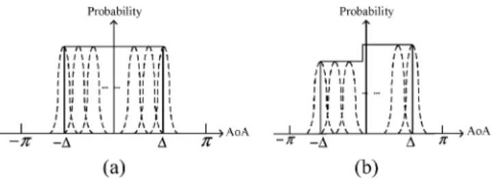
Fig. 1. AoA distribution of (a) uniform distribution over01 and 1 and (b) some specific distribution. The solid lines are the practical distribution curves, while the dotted lines are the sampling Gaussian distributions.
where N is the number of sampling Gaussian distribution, is the nth sampling mean AoA, and is the nth sampling stan-dard deviation. This approximation formulation combines many small angular-spread Gaussian distributions to fit a given large angle-spread uniform distribution as shown in Fig. 1(a). Using the small angular-spread approximate spatial correlation in [7], we may finally represent the spatial correlation as
(4)
This approximation can be extended to arbitrary AoA scenarios as shown in Fig. 1(b) as an example. For an AoA distribution that cannot be described by a mathematical formula easily, the discretized summation is needed for correlation evaluation. The approximation formulation we propose only samples specific mean AoAs over the distribution and uses the sampling Gaussian distributions to calculate the spatial correlation. Computation time of correlation calculation can thus be saved using the proposed approximation formulation. What should be mentioned is the weighting coefficients of the sampling Gaussian distributions may not equal 1/N and should be modified according to the AoA scenario. A simulation case in Section IV-A verifies the performance of our proposed approximation scheme.
III. PARAMETERIZED3-D SPATIALCORRELATION
Various definitions of antenna spatial correlation have been proposed in the literature [3]–[5]. In this section, a parameter-ized antenna spatial correlation formulation is presented, which takes individual 3-D antenna pattern and AoA scenarios into consideration. Essential parameters can be extracted from 3-D
antenna patterns and AoA distribution to represent the correla-tion.
Consider two antennas with mutual coupling, and the re-ceived signal vector of the two-element array can be shown as
(5) where and are the isolated antenna pattern
in theta and phi polarization, and is
the 3-D signal phase difference between two antenna elements. Moreover, and are the self-coupling and mutual coupling coefficient respectively suggested in [8]. The spatial correlation between two antennas is then defined as
(6) where is the 3-D AoA distribution in phi and theta polarization, and ( , 2) is the mean received power of the ith antenna defined as
(7)
Substitute (5) into (6) and (7), and the 3-D antenna spatial cor-relation is finally represented as (8), shown at the bottom of the page, where the lowercase is the coupling ratio whose value is equal to , is the expectation value of antenna pattern in terms of the AoA PDF, and are the real and imagi-nary part of spatial correlation for single antenna pattern without mutual coupling, and the subscript and are the value in theta and phi polarization, respectively. , , and are listed as
(9)
(10)
400 IEEE ANTENNAS AND WIRELESS PROPAGATION LETTERS, VOL. 8, 2009
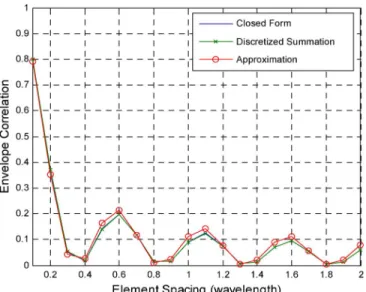
Fig. 2. Envelope correlation of the given AoA scenario.
(11) Furthermore, is defined as the envelope correlation that describes the effect of mutual coupling on the received power of two branches.
The presented spatial correlation in (8) shares the analogous form with the correlation in [3] but with the additional advan-tages. In [3], because the proposed spatial correlation belongs to the 2-D case, antenna polarization thus is not included in the definition of the spatial correlation. On the contrary, since (8) considers 3-D antenna patterns, it can further describe the polar-ization characteristic of the antennas. Moreover, the correlation only considers 2-D AoA distribution in [3], and it can be ob-served that various 3-D AoA distributions can be incorporated into the spatial correlation using (8).
The correlation formulation like (6) takes more computation time because, in commercial electromagnetic (EM) software, patterns are generated from the fields distributed on the antennas using near-field–far-field transformation. By contrast, the pro-posed spatial correlation extracts three parameters ( , , and ) to perform correlation calculation. As long as an isolated 3-D antenna pattern and the coupling matrix are obtained, the antenna spatial correlation can thus be computed rather than by recording the individual antenna pattern distorted by mutual coupling. Another important advantage of (8) is that the param-eterized correlation formulation can be combined with the pro-posed approximate correlation formulation in Section II to per-form a more efficient calculation. A simulation case and effi-ciency comparison will be presented in Section IV-B.
IV. SIMULATIONRESULTS
A. 2-D Spatial Correlation
We first show the performance of 2-D spatial correlation be-tween two ideal sources either by the conventional discretized
TABLE I
EFFICIENCYCOMPARISON OFDIFFERENTSCHEMES INFIG. 2
Fig. 3. The 3-D AoA distribution in Section IV-B.
summation or our approximation formulation. Simulation pro-grams are written in MATLAB and run on a PC with an Intel Pentium IV 3-GHz CPU. A uniformly distributed AoA scenario over is chosen as the benchmark. Moreover, to find a gauge to examine either the discretized summation or the approximation formulation performs correctly, the computation result of the numerical integration is regarded as the closed-form solution.
As from the work in [7], the approximate spatial correlation only fit well with the one calculated in either the closed-form or the discretized manner under the condition of small angular spread. For the value of angular spread larger than 20 , the ap-proximate spatial correlation may perform a less desirable re-sult. Therefore, each of the multiple Gaussian AoA distributions should also be chosen in the manner of small angular spread, and, in our case, is 2.5 in the confidence of accuracy. As soon as the angular spread of each sampling AoA distribution is deter-mined, we further make use of the characteristic of Gaussian dis-tribution where the values within two standard deviations from the mean are more than 95%. The sampling mean AoAs are thus chosen at every 5 , which are two standard deviations from the mean angle.
The correlations calculated by three different schemes in Fig. 2 share a similar curve trend with little variation. Numer-ical integration costs more time than the other two schemes, as shown in Table I; the main efficiency comparison is made between discretized summation and approximation formula-tion, and we find that the computation time of approximation formulation is 36% reduced compared to that of discreitized summation.
HSIEH AND CHEN: SPATIAL CORRELATION FORMULATION OF ARBITRARY AoA SCENARIOS 401
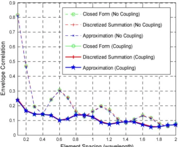
Fig. 4. 3-D envelope correlation.
B. 3-D Spatial Correlation With Antenna Mutual Coupling We further evaluate the derived 3-D spatial correlation be-tween two dipole antennas whose patterns are distorted by mutual coupling effect.
Two dipole antennas parallel to z-axis are located a distance d apart at y-axis. The single-dipole pattern and coupling matrix are generated from the EM software Ansoft HFSS. The 3-D AoA scenario for this case in Fig. 3 is a composite distribution that is an arbitrarily chosen dual-Gaussian-distributed PDF in phi-plane and a Gaussian distribution with mean 90 in theta-plane. We also assume all AoAs are in theta polarization so dipole antennas can receive all incident waves. Furthermore, because the approximation formulation in Section II belongs to the 2-D case, we only apply this method in phi-plane AoA distribution. As for theta-plane AoA distribution, we choose the discretized summation in advantage of its characteristic of small angle spread.
The computation result and efficiency of the spatial tion are shown in Fig. 4 and Table II, respectively. The
correla-TABLE II
EFFICIENCYCOMPARISON OFDIFFERENTSCHEMES INFIG. 4
tion values calculated by three different schemes share a similar trend again, and the computation time using approximation for-mulation is greatly reduced (more than 30%) compared to that using either numerical integration or discretized summation.
V. CONCLUSION
The approximation method we proposed in this letter is suit-able for the evaluation of the spatial correlation of arbitrary AoA scenarios. It can be applied to the 3-D parameterized spatial cor-relation formulation including antenna mutual coupling effect and reduce time complexity of correlation calculation.
REFERENCES
[1] G. J. Foschini and M. J. Gans, “On limits of wireless communications in a fading environment when using multiple antennas,” Wireless
Per-sonal Commun., vol. 6, pp. 311–355, 1998.
[2] S. Blanch, J. Romeu, and I. Corbella, “Exact representation of antenna system diversity performance from input parameter description,”
Elec-tron. Lett., vol. 39, no. 9, pp. 705–707, 2003.
[3] X. Li and Z. Nie, “Effect of mutual coupling on performance of MIMO wireless channels,” in Proc. ICMMT 4th Int. Conf., 2004, pp. 18–21. [4] C. Waldschmidt and W. Wiesbeck, “Compact wide-band multimode
antennas for MIMO and diversity,” IEEE Trans. Antennas Propag., vol. 52, no. 8, pp. 1963–1969, Aug. 2004.
[5] J. Fuhl, A. F. Molisch, and E. Bonek, “Unified channel model for mo-bile radio systems with smart antennas,” IEE Proc. Radar, Sonar
Nav-igation, vol. 145, no. 1, pp. 32–41, Feb. 1998.
[6] A. E. Zooghby, Smart Antenna Engineering. Norwood, MA: Artech House, 2005.
[7] R. M. Buehrer, “The impact of angular energy distribution on spatial correlation,” in Proc. IEEE 56th VTC Fall, 2002, vol. 2, pp. 24–28. [8] I. J. Gupta and A. A. Ksienski, “Effect of mutual coupling on the
perfor-mance of adaptive arrays,” IEEE Trans. Antennas Propag., vol. AP-31, no. 5, pp. 785–791, Sep. 1983.