國立交通大學
電子物理研究所
碩 士 論 文
開放式量子環中的量子傳輸
QUANTUM TRANSPORT THROUGH AN
OPEN QUANTUM RING
研 究 生:陳淑娟
指導教授:朱仲夏
開放式量子環中的量子傳輸
Quantum transport through an open quantum ring
研 究 生:陳淑娟 Student:
Shu-Chuan Chen指導教授:朱仲夏 Advisor:
Dr. Chon-Saar Chu國 立 交 通 大 學
電子物理研究所
碩 士 論 文
A Thesis
Submitted to Institute of Electrophysics College of Science
National Chiao Tung University in Partial Fulfillment of the Requirements
for the Degree of Master of Science in
Electrophysics January 2006
開放式量子環中的量子傳輸
研究生: 陳淑娟 指導教授: 朱仲夏 國立交通大學電子物理研究所摘要
本論文研究電子在開放式量子環中的傳輸特性。對於開放式量子環在零磁場時, 我們可以發現其共振態符合封閉環的束縛態。並且當兩邊通道(lead)不對稱或是 環的通道大小改變時,可以發現 Fano 結構。然而我們可以藉由改變環的對稱來 調整 Fano 結構使其由寬變窄,亦可以讓環的通道變寬而使得 Fano 結構由窄變 寬。在趨進一維的情形,共振峰變的較尖銳且向左移而接近封閉環的束縛態。對 於開放式量子環在有限磁場下,我們可以發現 AB 效應(Aharonov-Bohm effect) 而且其振盪周期為 Tp = Φ =2 0 h e/ 。然而值得注意的是在高磁場的情況下,並無 周期振盪的情形。假如我們改變兩邊通道的相對角度,我們可以發現在高磁場的 情況下改變角度變化較不大,但在低磁場的時候則是相反。Quantum transport through an open quantum ring
Stusent: Shu-Chuan Chen Advisors: Dr. Chon-Saar Chu Institute of Electro-physics
National Chiao Tung University
Abstract
We study quantum transport properties of an open quantum ring(OQR). For the OQR in zero magnetic filed, we have found that the resonant peaks correspond to the bond states of a close ring. Fano structure in the transmission of an OQR can be found in two case which the two lead are configured asymmetrically and the channel size of ring is changed. Moreover, we can tune the Fano structure from broad to sharp by varying the symmetry of OQR and tune the Fano structure from sharp to broad by widening the channel width of the ring. Then approaching to 1D case, the resonance peaks become shaper and shift toward the left to be close to bound of close ring, when the channel narrow down. For the OQR with finite magnetic filed, We have found that the AB effect when the external field are applied in the ring and the oscillating
periodTp = Φ =2 0 h e/ . And it should be noted that the periodic oscillations are
disappear at high magnetic field. If we change the angle θ of two lead for low and high magnetic field, we can found that it is sensitive to changing angle θ for small magnetic field but not for large magnetic field.
致謝
在我的研究所生涯裡,要誠摯的感謝朱老師的指導,不管是做研究的態度亦 或是在待人處事,老師都成為我很好的榜樣。此外,也特別謝謝唐志雄、鄔其君、 王律堯學長與鐘淑維學長在研究上給我許多幫助與提醒。最後要感謝實驗室同學 們,謝謝你們的陪伴與照顧。
Contents
Chinese Abstract I English Abstract II Acknowledgment III Content IV List of figures VI 1 introduction 1 1.1 Introduction . . . 1 1.2 Fano effect . . . 2 1.3 AB effect . . . 42 Theory and formulation 7
2.1 Landauer-Buttiker formalism . . . 7 2.2 Quantum transport through an open quantum ring with no magnetic field 9 2.3 Quantum transport through an open quantum ring in a magnetic field . . . 14 2.4 Quantum transport through an open quantum ring with a magnetic flux . 17 3 Result and discussion of open quantum ring without magnetic field 22 3.1 Mesoscopic transport properties of an open quantum ring . . . 22
CONTENTS
3.2.1 Effect of symmetrically to asymmetrically . . . 23 3.2.2 Effects of varying channel size of ring . . . 27 3.3 Approach to 1D rings . . . 27
4 Numerical results with finite magnetic field 32
4.1 Magnetic field character on quantum transport . . . 32 4.2 Momentum characteristics on quantum transport . . . 32
5 Numerical results with magnetic flux 38
5.1 Comparison with the 1D result . . . 38 5.2 Magnetic flux character on quantum transport . . . 38
List of Figures
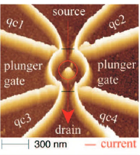
1.1 Micrograph of the quantum ring. The red line marks the current flow form source to drain through the two quantum point contacts angle the ring. The lateral gate electrodes termed qc1-qc4 are used to tune the tunnel barriers (indicate by dotted lines) connecting the quantum ring to its leads. The plunger gates allow the electron number on the ring to be controlled (adapted from Ref. 9) . . . 3 1.2 Transmission-electron micrograph of ring-shaped conductor [6]. The inside
diameter of loop is 784 nm and the width of the wires is 41 nm (adapted from Ref.6).) . . . 5 1.3 (a)Magnetoresistance of the above ring measured at T = 0.01K. (b)Fourier
power spectrum in arbitrary units containing peaks at h/e and h/2e (adapted from Ref.6). . . 5 1.4 Aharonov-Bohm ring. . . 6 2.1 Schematic illustration of the ring . . . 9 3.1 The solid line refers transmission probabilities as functions of the electron
momentum for an OQR of r2 = 2, r1 = 1, s = 1 and θ = π. The dashed
line refers the momentum of confined states in the closed ring. The n and
m is the radial and angular quantum number, respectively. . . 24
LIST OF FIGURES
3.3 Current transmission as a function of the electron momentum of the OQR of r2 = 2, r1 = 1, s = 1, for different angle θ = π(a), 0.99π(b), 0.98π(c),
0.97π(d), 0.96π(e), 0.95π(f). . . 26 3.4 The solid line is transmission probabilities as functions of the electron
mo-mentum of the OQR of r1 = 1, s = 1 and θ = π, for different r2 = 1(a),
0.99(b), 0.98(c), 0.97(d), 0.96(e), 0.95(f). . . 28 3.5 The solid line is transmission probabilities as functions of (L1+ L2)/λ// of
the OQR of θ = π, for (a)R/s = 3.5, (b)R/s = 9.5 . . . 29 3.6 The solid line is transmission probabilities as functions of (L1 + L2)/λ//
of the OQR for (a)R/s = 3.5, L1/L2 = 0.9 (b)R/s = 9.5, L1/L2 = 0.9,
(c)R/s = 3.5, L1/L2 = 0.7, (d)R/s = 3.5, L1/L2 = 0.7 . . . 31
4.1 The transmission probability as a function of Φ/Φ0 for an AB ring, the
parameters r2 = 2, r1 = 1, θ = π and k = 1.182. . . 33
4.2 The transmission of an OQR in weak magnetic field (Φ/Φ0 = 0.48,
dash-dotted line) and in zero magnetic field (Φ/Φ0 = 0, solid line) . . . 35
4.3 The transmission of an OQR r2 = 2 and r1 = 1 in lower magnetic field
(Φ/Φ0 = 0.48)for different θ = π(solid line), 0.96π(dotted line), 0.92π(dashed
line). . . 36 4.4 The transmission as a function of momentum k. The parameters are r2 = 2,
r1 = 1,and k = 1.182 in higher magnetic field (Φ/Φ0 = 9.87)for different
θ = π(solid line), 0.97π(dash-dotted line), 0.8π(dashed line). . . 37
5.1 The transmission probability T is plotted versus the dimensionless lon-gitudinal wave number in Q1D scheme (r2 = 4, r1 = 3, solid line) and
1D(r = 3.5, dash line) scheme [24], for different flux Φ/Φ0 =(a)2.0, (b)1.6,
LIST OF FIGURES
5.2 The transmission probability as a function of Φ/Φ0 for an OQR with a
magnetic flux in center of ring , the parameters r2 = 2, r1 = 1, θ = π and
k = 1.11. . . 40
5.3 The wave function of Φ/Φ0= (a)12.93, (b)13.21, (c)14.97, (d)15.21, (e)15.09,
Chapter 1
introduction
1.1
Introduction
In the past decade developments in mesoscopic physics have received much attention and made rapid progress. Quantum transport in the mesoscopic systems has been extensively studied both experimentally and theoretically. And the atomlike properties of dots or gate-confined quantum make them a good venue for studying the physics of confined carriers and many-body effects. Hence quantum dots have attracted considerable interest due to its potential to various application. They lead to interesting applications in fields such as quantum cryptography, quantum computing, optics, and optoelectronics, etc.
In recent work, however, a new geometry of semiconductor quantum rings has been introduced in experiments of magnetocapacitance and infrared excitation for few electrons [1, 2]. In many aspects, quantum rings are just quantum dots with a peculiar confining potential [3]. The decisive difference in their topology that the hole in their middle becomes prominent when an external magnetic field is applied. The magnetic flux that penetrates the interior of the ring will then determine the nature of the electronic states. Since the pioneering publications in Ref.4, 5, the theoretical and experimental studies of ring interferometers are studied extensively. In ring geometries strongly connected to external leads the electron wave packets can take two different paths around the ring
CHAPTER 1. INTRODUCTION
which gives rise to interference. This can be associated with Young’s double-slit ex-periment for photons. The electron in a ring geometry allows the relative phase of the electronic wave function in the two arms of the ring to be manipulated by a magnetic field perpendicular to the plane of the ring. And Aharonov and Bohm proposed such a setup to test experimentally the significance of the magnetic vector potential in quantum mechanics [6]. They predicted that the phase difference of the alternative paths changes by 2π as the flux through the ring is changed by one flux quantum h/q (q is the charge of the particle). Then magnetic field periodic resistance oscillations in ring structure have demonstrated that have a phase coherence length longer than or comparable to the perimeter by many experiments. Hence in mesoscopic physics the Aharonov-Bohm (AB) effect has become a standard tool to quantitatively investigate the phase coherence of transport in either metallic [7] or semiconducting systems [8–10]. Figure 1.1 shows the topography of a GaAs-AlGaAs heterostructure containing a two-dimensional electron gas below the surface.
In this thesis we study quantum transport properties of an open quantum ring(OQR). For simplicity, we ignore the effects of spins and the mutual interactions. Then we can found some interesting phenomena. If we change geometric configuration from symmet-rical to asymmetsymmet-rical of OQR, the Fano structures can be found in the transmission. Moreover the AB effect also can be observe in transmission of OQR with magnetic field. In the following , we would introduce the Fano effect and AB effect.
1.2
Fano effect
In 1961, Fano considered a physical situation which occurs in many systems addressed spectroscopically [11]. In the first part of the calculation, a quantum state, |φi , with energy E0
φ, is taken to be coupled via matrix elements VE0 to a continuum of states denoted
CHAPTER 1. INTRODUCTION
Figure 1.1: Micrograph of the quantum ring. The red line marks the current flow form source to drain through the two quantum point contacts angle the ring. The lateral gate electrodes termed qc1-qc4 are used to tune the tunnel barriers (indicate by dotted lines) connecting the quantum ring to its leads. The plunger gates allow the electron number on the ring to be controlled (adapted from Ref. 9)
CHAPTER 1. INTRODUCTION
considered, and it is shown that the interference between the contributions of the original continuum states and the resonance will always yields a characteristic asymmetric line shape in the transition probability. The typical phenomenon of Fano structures in which the transmission probabilities is downward dips to zero and soon rise up to one.
The Fano effect, a ubiquitous phenomenon observed in a large variety of experiments including neutron scattering [12], atomic photoionization [13], Raman scattering [14], and optical absorption [15]. While a statistically averaged nature of the system containing contributions from numerous sites is observed in these experiments, the Fano effect is essentially a single-impurity problem describing how a localized state embedded in the continuum acquires itinerancy over the system [16]. Therefore, an experiment on a single site would reveal this fundamental process in a more transparent way. While the single-site Fano effect has been reported in the scanning tunneling spectroscopy study of an atom on the surface [17, 18] or in transport through a quantum dot (QD) [19], there is little, if any, controllability in either case since the coupling between the discrete level and the continuum is naturally formed.
1.3
AB effect
According to quantum physics, when two coherent electron waves travelling along distinct paths recombine, they will interfere. The outcome reflects a phase difference arising from the different lengths of the paths taken by the electrons. If a magnetic field penetrates the region between the two paths, it will cause an additional phase shift, and so will change the resulting interference - a phenomenon known as the Aharanov-Bohm effect [6]
In this section, we would discuses the Aharonov-Bohm (AB) effect for a ring-shaped conductor. Experimentally [8, 9], the conductance of the ring have been observed to oscillate as a function of the magnetic through the ring, see Fig. 1.2and Fig. 1.3. The fundamental period of the oscillations is found to be the flux quantum, Φ0 = h/e.
CHAPTER 1. INTRODUCTION
Figure 1.2: Transmission-electron micrograph of ring-shaped conductor [6]. The inside diameter of loop is 784 nm and the width of the wires is 41 nm (adapted from Ref.6).)
Figure 1.3: (a)Magnetoresistance of the above ring measured at T = 0.01K. (b)Fourier power spectrum in arbitrary units containing peaks at h/e and h/2e (adapted from Ref.6).
CHAPTER 1. INTRODUCTION
The oscillations are caused by interference between the waves traversing the two branches of the ring (see Fig. 1.4).
Figure 1.4: Aharonov-Bohm ring.
The phase shift in the upper branch of the ring is
θup= |e| ~ Z 2 1 − → A · d−→r (1.1)
The fundamental period of the oscillations is found to be the flux quantum Φ0 = |e|~. By
choosing in cylindrical coordinates −→A = 1
2Br−u→φ we obtain for the phase shift θup = πΦΦ0
where Φ is the total flux through the ring. Similarly, the phase shift in the lower branch is θlow = −πΦΦ0.
The total phase difference between the waves in the different branches on the r.h.s. of the ring is thus θ = 2πΦ
Φ0. Consequently, the transmission probability oscillates with the
period Φ0. For example, if there is only one mode propagating in the ring, the transmission
probability vanishes every time the phase shift equals an odd multiple of π.
In addition to the h/e-oscillations, there can also be observed subharmonic oscillations with frequencies h/ne, where n is an integer. These are caused by the waves traversing n times half of the ring in the same direction before interfering (now the total phase shift of the waves traversing, for example, in the clockwise direction is π Φ
Chapter 2
Theory and formulation
2.1
Landauer-Buttiker formalism
When the characteristic sizes of semiconductor devices are small in comparison with the elastic mean free path of carriers, the carrier transport becomes ballistic [20]. The Landauer-Buttiker formalism, which treats the transport as a scattering process, is par-ticular useful for the description of transport thought a mesoscopic system in the ballistic transport regime. And in this section, we introduce the multchannel Landauer-Buttiker formalism starting from the single channel case [4].
Assume that there are two reservoir of electrochemical potential µ1 and µ2 respectively
connected by a 1D channel and there is a barrier in between the reservoirs. Consider two reservoirs having the difference δµ = µ1− µ2 in the electrochemical potential. We assume
that electron coming into both side reservoirs form the 1D channel will not reflect back. So, only those transmitted electrons in between δµ contribute to the current density J from reservoir 1 to 2 in 1D, J=I.
In order to calculate the conductance we start from the equation of the current density at zero temperature
CHAPTER 2. THEORY AND FORMULATION
where vF indicates Fermi velocity, n is the number of states per unit length that injected from reservior 1 to reservoir 2, and considering the probability for transmission to be T,
n can be written as n = µ dN dE ¶ (µ1− µ2) T (2.2)
For the density of state with 2 spin-states included, (dN/dE) = 2/vF in a 1D system (only one of the propagating direction is counted). Hence, we have
I = −2e
h δµT (2.3)
Since the voltage difference δV = δµ/(−e) , so that the conductance is in the form
G = 2e
2
h T (2.4)
For the case of multichannel system, we consider that electron propagate from the left nth subband transmitted into right mth subband, and assume the transmission probability as
Tnm, and the reflection probability as Rnm.Therefore, the total transmission probability
Tn and the total reflection probability Rn from the nth channel is
Tn = P m Tnm Rn = P m Rnm (2.5)
By definition, the total current should be taken into account the contribution of all the incident subbands, Itot =
P n
In, where the In is related to the current transmission Tn, so we have In = − 2e h δµ X m Tnm (2.6)
CHAPTER 2. THEORY AND FORMULATION and Itot = − 2e hδµ X n X m Tnm (2.7)
Following the Landaner-Buttiker formalism, the conductance can be expressed of the form
G = 2e2 h X n X m Tnm (2.8)
2.2
Quantum transport through an open quantum
ring with no magnetic field
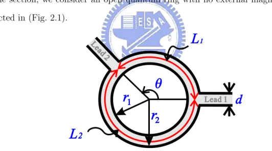
In the section, we consider an open quantum ring with no external magnetic field, as is depicted in (Fig. 2.1).
r
1r
2 Lead 1 L ead 2d
L
1L
2Figure 2.1: Schematic illustration of the ring
In the ring region, the Hamiltonian describing an electron inside the ring can be written of the form H = ~2 2m∗ · − ∂2 ∂r2 − 1 r ∂ ∂r − 1 r2 ∂2 ∂θ2 ¸ + Vr(r) (2.9)
CHAPTER 2. THEORY AND FORMULATION
this case we adopt a hard-wall laterally confined model, namely,
Vr(r) = 0,r1 ≤ r ≤ r2 ∞,r > r2, r < r1 (2.10)
And then we choose the energy unit E∗ = ~2k2
F/2m∗, the length unit a∗ = 1/kF. Thus we can obtain the dimensionless Schrodinger Equation for ring:
· − ∂2 ∂r2 − 1 r ∂ ∂r − 1 r2 ∂2 ∂θ2 + Vr(r) ¸ ψr(r, θ) = Eψr(r, θ) (2.11)
Here kF is a typical Fermi wave vector in the reservoirs.
Taking the same units, we also can obtain the dimensionless Schrodinger Equation for leads as · − ∂2 ∂x2 − ∂2 ∂y2 + VL(y) ¸
ψ(i)L (x, y) = EψL(i)(x, y) (2.12)
VL(y) = 0, 0 ≤ y ≤ d ∞,y < 0, y > d
where i = 1 for lead 1, i = 2 for lead 2, VL(y) is the confinement potential, and d is the width of lead.
By solve the Eq. (2.11) and Eq. (2.12), hence we can write down the wave function in each region: ψL(1)(x, y) = PN n=1 (a(1)n eiknx+ b(1)n e−iknx) q 2 dsin nπy d , ψr(r, θ) = √12π M P m=−M cmφm(kr)eimθ ψL(2)(x, y) = PN n=1 (a(2)n eiknx+ b(2)n e−iknx) q 2 dsin nπy d (2.13)
CHAPTER 2. THEORY AND FORMULATION and ∂ψ(1)L /∂x = PN n=1
(ikn)(a(1)n eiknx− b(1)n e−iknx) q 2 dsin nπy d ∂ψr/∂r = √12π M P m=−M cmφ0m(kr)eimθ ∂ψ(2)L /∂x = PN n=1
(ikn)(a(2)n eiknx− b(2)n e−iknx) q 2 dsin nπy d (2.14)
where n, m are both subband indices in the leads and the ring respectively. For the region of lead, d is the width of lead and the transverse energy levels are quantized, with
En= n2π2/d2, so the wave vector for an electron with energy E and in the nth subband is given by kn=
√
E − En. For the region of ring, φm(kr) is the radial wave function,
φm(kr) = Jm(kr) + αmYm(kr) (2.15)
where k =√E, and Jm(kr) and Ym(kr) are the Bessel functions of first and second kinds, respectively. Here φm(kr) satisfies the boundary condition φm(kr1) = 0, and hence
αm = −Jm(kr1)/Ym(kr1) (2.16)
Now, by matching the wave function for the boundary conditions:
ψL(1)(0, y) + ψL(2)(0, y) = ψr(r2, θ) (2.17) ∂ψL(1)/∂x ¯ ¯ ¯ x=0 = ∂ψr/∂r|r=r2 (2.18) ∂ψL(2)/∂x ¯ ¯ ¯ x=0 = ∂ψr/∂r|r=r2 (2.19)
If we neglect the difference between the straight line of the channel and the arc line of the ring, and the angles to which the two side of two leads are θ1, θ2 and θ3, θ4 respectively,
CHAPTER 2. THEORY AND FORMULATION hence we have N P n=1 (a(1)n + b(1)n ) q 2 dsin nπr2(θ−θ1) d + N P n=1 (a(2)n + b(2)n ) q 2 dsin nπr2(θ−θ3) d = √1 2π M P m=−M cmφm(kr)eimθ (2.20) N X n=1 (ikn)(a(1)n − b(1)n ) r 2 dsin nπr2(θ − θ1) d = 1 √ 2π M X m=−M cmφ0m(kr)eimθ (2.21) N X n=1 (ikn)(a(2)n − b(2)n ) r 2 dsin nπr2(θ − θ3) d = 1 √ 2π M X m=−M cmφ0m(kr)eimθ (2.22) In the first stage, let us multiply both sides of Eq. (2.20) by the factor (1/√2π)e−im0θ
. Here m0 = 0, ±1, ±2 · · · ± M, and integrate from zero to 2π,
N X n=1 (a(1) n + b(1)n )I−m0n+ N X n=1 (a(2) n + b(2)n ) ˜I−m0n= cm0φm0(kr2), m0 = 0, ±1, ±2, ..., ±M (2.23)
Then, we multiply both sides of Eq. (2.21) and Eq. (2.22) by p2/d sin n0πr
2(θ − θ1)/d
and p2/d sin n0πr
2(θ − θ3)/d , respectively. Here n0 = 1, 2 · · · N , and integrate from θ1
to θ2, N X n=1 (ikn)(a(1)n − b(1)n )Un0n = M X m=−M cmφ0m(kr2)Imn0, n0 = 1, 2, ..., N (2.24) N X n=1 (ikn)(a(2)n − b(2)n ) ˜Un0n = M X m=−M cmφ0m(kr2) ˜Imn0, n0 = 1, 2, ..., N (2.25) where I±mn = r 1 πd Z θ2 θ1 sinnπr2(θ − θ1) d e ±imθdθ (2.26) r 1 Z θ4 nπr (θ − θ )
CHAPTER 2. THEORY AND FORMULATION Un0n = 2 d Z θ2 θ1 sinn 0πr 2(θ − θ1) d sin nπr2(θ − θ1) d dθ (2.28) ˜ Un0n = 2 d Z θ4 θ3 sinn 0πr 2(θ − θ3) d sin nπr2(θ − θ3) d dθ (2.29)
In Eq. (2.13) b(1)n and b(2)n are coefficients of electron waves traveling inward or increasing exponentially with x (for imaginary kn), which are all set to be zero according to physical consideration, except one coefficient b(1)i = 1/√ki, representing the amplitude of one injected wave. And the coefficients a(1)n and a(2)n which are related to the transmission and reflection amplitudes. Hence we have 2M+2N+1 equations Eq. (2.23)-Eq. (2.25) for 2M+2N+1 unknown coefficients a(1)n , a(2)n (n0 = 1, 2, ...N)and cm(m = 0, ±1, ... ± M).
Rewrite the Eq. (2.23)-Eq. (2.25) in matrix form
I0(A + B) + ˜I0(A0 + B0) = ΦC (2.30)
iUK(A − B) = I1Φ0C (2.31)
i ˜UK(A0− B0) = ˜I1Φ0C (2.32)
where
Solving the set of equations we obtain the coefficients a(1)n and a(2)n :
a(1) n = rni √ kn (2.33) a(2) n = tni √ kn (2.34) The total transmission and reflection probabilities are given by
T =P ni |tni|2 R =P ni |rni|2 (2.35)
CHAPTER 2. THEORY AND FORMULATION
Moreover, the conductance G can be found by the expression
G = 2e2
h T (2.36)
2.3
Quantum transport through an open quantum
ring in a magnetic field
In the section, we consider an open quantum ring applied by an external perpendicular magnetic field, while the two leads without magnetic field.
In the region of ring, the Hamiltonian of an electron in a ring with a magnetic field B is given by H = 1 2m∗(P + eA) 2+ V r(r) = 1 2m∗(P2+ e (P · A + A · P) + e2A2) + Vr(r) (2.37)
where m* is the effective mass of electron, Vr(r) is the radial confining potential. In this case, again, we consider the ring with hard-wall confinement described by
Vr(r) = 0,r1 ≤ r ≤ r2 ∞,r > r2, r < r1 (2.38)
and A is the magnetic vector potential such that B = ∇ × A.
Assuming that the magnetic field is constant and perpendicular to the plane of the ring, the vector potential can be expressed in polar coordinates:
A = B
2 (0, r, 0) (2.39)
CHAPTER 2. THEORY AND FORMULATION Hamiltonian in polar coordinates
H = ~2 2m∗ " − µ ∂2 ∂r2 + 1 r ∂ ∂r + 1 r2 ∂2 ∂θ2 ¶ − ieB ~ µ ∂ ∂θ ¶ + 1 ~2 µ eB 2 ¶2 r2 # + Vr(r) (2.40)
Let wc= eBm∗ , wc being the cyclotron frequency, and then the Hamiltonian can be rewrite of the form H = ~2 2m∗ · − µ ∂2 ∂r2 + 1 r ∂ ∂r + 1 r2 ∂2 ∂θ2 ¶ − i1 ~m ∗w c µ ∂ ∂θ ¶ + 1 ~2 1 4(m ∗)2w2 cr2 ¸ +Vr(r) (2.41)
And then we choose the energy unit E∗ = ~2k2
F/2m∗, the length unit a∗ = 1/kF, and
w∗
c = E∗/~ = ~kF2/2m∗. Therefore we can obtain the dimensionless Schrodinger equation describing the electronic transport through the open quantum ring, given by
· − µ ∂2 ∂r2 + 1 r ∂ ∂r + 1 r2 ∂2 ∂θ2 ¶ −i1 2wc µ ∂ ∂θ ¶ + 1 16(wc) 2r2+ V r(r) ¸ ψr(r, θ) = Eψr(r, θ) (2.42)
Assuming the eigenfunction can be written as
ψr(r, θ) =
eimθ
√
2πRm(r) (2.43)
Substituting Eq. (2.43) into Eq. (2.42), we have · − µ ∂2 ∂r2 + 1 r ∂ ∂r ¶ + µ m2 r2 ¶ +1 2mwc+ 1 16(wc) 2r2 ¸ Rm(r) = ERm(r) (2.44) ⇒ ·µ ∂2 ∂r2 + 1 r ∂ ∂r ¶ − µ m2 r2 ¶ + µ E −1 2mwc ¶ − 1 16(wc) 2r2 ¸ Rm(r) = 0 (2.45) Then we assume Rm(r) ∼ r|m|e−(wcr 2)/8 u(r) = r|m|e−ar2 u (r) (2.46)
CHAPTER 2. THEORY AND FORMULATION here a = wc/8.
Substituting Eq. (2.46) into Eq. (2.45), we can obtain n ∂2u(r) ∂r2 + ¡ (2 |m| + 1) r−1+¡−wc 2 ¢ r¢∂u(r)∂r + £ (2 |m| + 2)¡−wc 4 ¢ +¡E − 1 2mwc ¢¤ª u(r) = 0 (2.47)
Now, let x = 2ar2=wc
4 r2 , so we get ∂x ∂r = wcr/2 (2.48) ∂2x ∂2r = wc/2 (2.49) ∂u(r) ∂r = ∂x ∂r du(x) dx = wc 2 r du(x) dx (2.50) ∂2u(r) ∂r2 = ∂2x ∂2r du(x) dx + µ ∂x ∂r ¶2 d2u(x) dx2 = wc 2 du(x) dx + ³wc 2 ´2 r2d 2u(x) dx2 (2.51)
Substituting Eq. (2.48)-Eq. (2.51) into Eq. (2.47), we have xd2u(x) dx2 + {((|m| + 1) − x) } du(x) dx + ·µ E wc − 1 2 mwc wc ¶ −1 2(|m| + 1) ¸ | {z } εm u(x) = 0 (2.52) where εm = µ E wc − 1 2m ¶ −1 2(|m| + 1) (2.53)
Eq. (2.52) is the form of confluent hypergeometric equation, namely that the u(x) is the so-called confluent hypergeometric function, give by
u(x) = cmM(−εm, |m| + 1; wc 4 r 2) + d mU(−εm, |m| + 1; wc 4 r 2) (2.54)
CHAPTER 2. THEORY AND FORMULATION
It is now easy to obtain the R (r) by substituting Eq. (2.54) into Eq. (2.46):
Rm(r) = r|m| ¡ cmM(−εm, |m| + 1;w4cr2) + dmU(−εm, |m| + 1; w4cr2) ¢ e−wcr2/8 =cmr|m| ¡ M(−εm, |m| + 1; w4cr2) + αmU(−εm, |m| + 1;w4cr2) ¢ e−wcr2/8 =cmφm(r) (2.55)
where M , U are the confluent hypergeometric functions of first and second kinds, re-spectively. The Rm(r) satisfies the boundary condition Rm(r1) = 0, and hence
αm = −M(−εm, |m| + 1; wc 4 r 2 1)/U(−εm, |m| + 1; wc 4 r 2 1) (2.56)
Hence the wavefunction which in the region of ring is written as
ψr(r, θ) = 1 √ 2π X m cmφm(r)eimθ (2.57)
Utilizing this equation, itis easy to caculate the total transmission and reflection proba-bilities of the open ring system by matching boundary condition which is the same as the method in Sec. 2.2.
2.4
Quantum transport through an open quantum
ring with a magnetic flux
In the section, we consider an open quantum ring with a magnetic flux in center of ring. Assuming that the magnetic flux is constant and in the center region of ring, the vector potential can be expressed :
Aϕ = Φ/2πr Ar = 0 Az = 0 (2.58)
CHAPTER 2. THEORY AND FORMULATION Hamiltonian: H = 1 2m∗(P + eA) 2+ V r(r) = 1 2m∗(P2+ e (P · A + A · P) + e2A2) + Vr(r) (2.59)
where m* is the effective mass of electron, Vr(r) is the radial confining potential. In this case, again, we consider the ring with hard-wall confinement described by
Vr(r) = 0,r1 ≤ r ≤ r2 ∞,r > r2, r < r1 (2.60)
Since the system is circularly symmetric it is convenient to write the Hamiltonian in polar coordinates: H = ~ 2 2m∗ " − µ ∂2 ∂r2 + 1 r ∂ ∂r + 1 r2 ∂2 ∂θ2 ¶ − i2e ~ µ Φ 2πr 1 r ∂ ∂θ ¶ + µ e ~ Φ 2πr ¶2# + Vr(r) (2.61) Let α=e
~2πΦ = 2ΦΦ0 , Φ being the magnetic flux, and defining Φ0 =
h
2e as the flux
quantum, then the Hamiltonian can be rewrite of the form
H = − ~2 2m∗ · ∂2 ∂r2 + 1 r ∂ ∂r + 1 r2 µ ∂2 ∂θ2 + i2α ∂ ∂θ − α 2 ¶¸ + Vr(r) (2.62)
And then we choose the energy unit E∗ = ~2k2
F/2m∗, and the length unit a∗ = 1/kF. Therefore we can obtain the dimensionless Schrodinger equation describing the electronic transport through the open quantum ring, given by
· − µ ∂2 ∂r2 + 1 r ∂ ∂r + 1 r2 µ ∂2 ∂θ2 + i2α ∂ ∂θ − α 2 ¶¶ + Vr(r) ¸ ψr(r, θ) = Eψr(r, θ) (2.63)
Eq. (2.63) can be rewritten as µ r2 ∂2 + r ∂ + r2(E − V r(r)) ¶ ψr(r, θ) = − µ ∂2 + i2α ∂ − α2 ¶ ψr(r, θ) (2.64)
CHAPTER 2. THEORY AND FORMULATION Assuming the eigenfunction can be written as
ψr(r, θ) = R(r)Θ(θ) (2.65)
Substituting Eq. (2.65) into Eq. (2.64), we have 1 R(r) µ r2 ∂2 ∂r2 + r ∂ ∂r + r 2(E) ¶ R(r) = − 1 Θ(θ) µ ∂2 ∂θ2 + i2α ∂ ∂θ − α 2 ¶ Θ(θ) (2.66) First,we let − 1 Θ(θ) µ ∂2 ∂θ2 + i2α ∂ ∂θ − α 2 ¶ Θ(θ) = d2 (2.67) and assume Θ(θ) = √1 2πe i(m0−α)θ (2.68)
Substituting Eq. (2.68) into RHS of Eq. (2.67):
− 1 ei(m0−α)θ ³ ∂2 ∂θ2 + i2α∂θ∂ − α2 ´ ei(m0−α)θ = − 1 ei(m0−α)θ ¡ (i (m0− α))2ei(m0−α)θ + i2α (i (m0− α)) ei(m0−α)θ − α2ei(m0−α)θ¢ = −¡(i (m0− α))2+ i2α (i (m0− α)) − α2¢ = − (− (m02− 2m0α + α2) − 2m0α + 2α2− α2) = − (−m02) = m02 (2.69) hence, d2 = m02.
The boundary condition of Θ(θ) is
CHAPTER 2. THEORY AND FORMULATION Substituting Eq. (2.68) into Eq. (2.70), we can obtain
ei(m0−α)2π
= 0 (2.71)
Hence, m0− α = 0, ±1, ±2 · · · ± M. Then Eq. (2.66) can be rewritten as
1 R(r) µ r2 ∂2 ∂r2 + r ∂ ∂r + r 2(E) ¶ R(r) = m02 (2.72) For any m0 µ r2 ∂2 ∂r2 + r ∂ ∂r + r 2E − m02 ¶ Rm0(r) = 0 (2.73)
Now, let k =√E and t = kr, so Eq. (2.73) become ∂2R m0(t) ∂t2 + 1 t ∂Rm0(t) ∂t + (1 − m02 t2 )Rm0(t) = 0 (2.74)
Eq. (2.74) is the form of bessel equation, hence Rm0(kr) give by
Rm0(kr) = cm0(Jm0(kr) + αm0Nm0(kr)) , m0 = 0, ±1, ±2 · · · ± M cm0(Jm0(kr) + αm0J−m0(kr)) , other (2.75)
where Jm0(kr) and Ym0(kr) are the Bessel functions of first and second kinds, respectively.
Here Rm0(kr) satisfies the boundary condition Rm0(kr1) = 0, and hence
αm0 = −Jm0(kr1)/Nm0(kr1), m0 = 0, ±1, ±2 · · · ± M −Jm0(kr1)/J−m0(kr1), other (2.76)
CHAPTER 2. THEORY AND FORMULATION
Let m0 − α = m = 0, ±1, ±2, L, ±M, so Eq. (2.75) become
Rm0(kr) = cm(Jm+α(kr) + αmNm+α(kr)) , m + α = 0, ±1, ±2 · · · ± M cm ¡ Jm+α(kr) + αmJ−(m+α)(kr) ¢ , other = cmφm+α(kr) (2.77)
Hence the wavefunction which in the region of ring is written as
ψr(r) = R(r)Θ(θ) = 1 √ 2π M X m=−M cmφm+α(kr)eimθ (2.78)
Utilizing this equation, it is easy to calculate the total transmission and reflection proba-bilities of the open ring system by matching boundary condition which is the same as the method in Sec. 2.1.
Chapter 3
Result and discussion of open
quantum ring without magnetic field
We already derive the transmission probabilities of an open quantum ring (OQR) match-ing method. And the electronic transmission and the electron wave function can be exactly calculated numerically. In this chapter, we would like to show our results of electronic transport through an OQR of r2 = 2, r1 = 1, s = 1. And then we vary the angle (θ) of
the two lead and the channel size of ring, the result are shown in the section 3.2. Finally, we approach our result to 1-D case.
3.1
Mesoscopic transport properties of an open
quan-tum ring
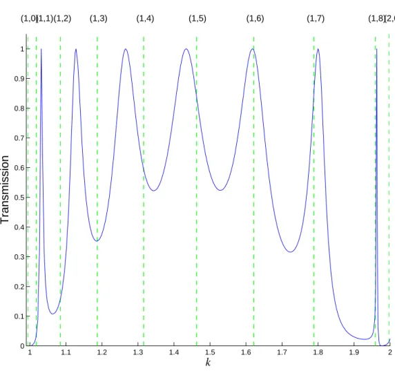
The coefficient of electron transmission through the open quantumnh ring in zero magnetic field was calculated in Chap.2. As shown in Fig. 3.1, the transmission probabilities T (solid line) as a functions of the momentum of injected electron for an OQR of r2 = 2,
r1 = 1, s = 1 and θ = π. Here, we just consider the momentum of the range from 1 to
CHAPTER 3. RESULT AND DISCUSSION OF OPEN QUANTUM RING WITHOUT MAGNETIC FIELD
ring. Here, n and m are the radial and angular quantum number, respectively.
In Fig. 3.1, for the solid line, there are seven peaks and dips, the maximum value is one for each peak and the minimum value of dip is form of envelope. And the momentum of those peaks are 1.032, 1.127, 1.266, 1.434, 1.618, 1.80 and 1.96, the momentum of those dip are 1.063, 1.185, 1.344, 1.529, 1.723, 1.929 and 1.977. And for the dashed line, there are eight confined states of close ring, we denote them as (n,m) = (1,1)(1,2)...(1,8), respectively.
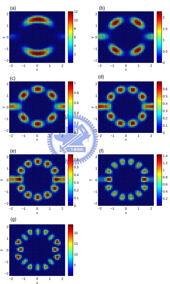
From the Fig. 3.1, we observe that the peaks are sharper and they also match better with confined states when the momentum k are near the subband of lead (k =1,2). And we can found that there are eight dashed line, but there are only seven peaks, it seems that one peak in the transmission is missing. In order to understand the incident electron behavior in space, hence we plot wave function probability at the maximum value of peak. They are shown in Fig. 3.2. Comparing Fig. 3.2(a)-(g), we can found that the wave function at k = 1.032(a), 1.127(b), 1.266(c) and 1.344(d), the number of waves in the ring are 1, 2, 3 and 4, respectively. And directly perceived through the senses, it seems that the number of waves in the ring at k =1.618(e) shall be 5 by sense, but from the Fig. 3.2(e), we can see that there are 6 waves in the ring at k =1.618. So we can know that the peak of missing shall between k =1.4339 and 1.618. And the scale of wavefunctioin probability in the ring for k =1.032 and 1.8 are larger than lead. However, it seems that the electron like to stay in the ring relatively.
3.2
Tuning of the Fano resonance in an open
quan-tum ring
3.2.1
Effect of symmetrically to asymmetrically
Fano structure in the transmission of an OQR can be found in two case which the two lead are configured asymmetrically and the channel size of ring is changed. First, we consider
CHAPTER 3. RESULT AND DISCUSSION OF OPEN QUANTUM RING WITHOUT MAGNETIC FIELD
1 1.1 1.2 1.3 1.4 1.5 1.6 1.7 1.8 1.9 2 0 0.1 0.2 0.3 0.4 0.5 0.6 0.7 0.8 0.9 1 k Transmission (1,1)(1,2) (1,3) (1,4) (1,5) (1,6) (1,7) (1,8)(2,0) (1,0)
Figure 3.1: The solid line refers transmission probabilities as functions of the electron momentum for an OQR of r2 = 2, r1 = 1, s = 1 and θ = π. The dashed line refers the
momentum of confined states in the closed ring. The n and m is the radial and angular quantum number, respectively.
CHAPTER 3. RESULT AND DISCUSSION OF OPEN QUANTUM RING WITHOUT MAGNETIC FIELD
−2 −1 0 1 2 −2 −1 0 1 2 x y −2 −1 0 1 2 −2 −1 0 1 2 x y −2 −1 0 1 2 −2 −1 0 1 2 x y −2 −1 0 1 2 −2 −1 0 1 2 x y 2 4 6 8 10 12 0 0.5 1 1.5 2 0 0.2 0.4 0.6 0.8 1 0 0.1 0.2 0.3 0.4 0.5 0.6 (a) (b) (c) (d) −2 −1 0 1 2 −2 −1 0 1 2 x y −2 −1 0 1 2 −2 −1 0 1 2 x y −2 −1 0 1 2 −2 −1 0 1 2 x y 0 0.1 0.2 0.3 0.4 0.5 0.6 0.2 0.4 0.6 0.8 1 1.2 1.4 5 10 15 20 (e) (f) (g)
Figure 3.2: The wave function of k =1.032(a), 1.127(b), 1.266(c), 1.434(d), 1.618(e), 1.8(f), 1.96(g) for r2 = 2, r1 = 1, s = 1 and θ = π
CHAPTER 3. RESULT AND DISCUSSION OF OPEN QUANTUM RING WITHOUT MAGNETIC FIELD
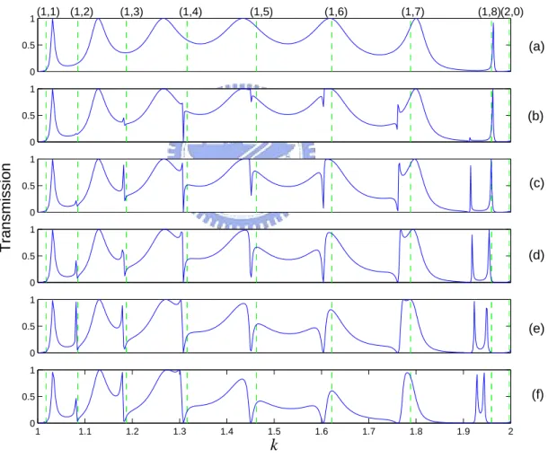
the case that two lead are configured asymmetrically, that is shown in Fig. 3.3 From Fig. 3.3, we see that the typical phenomenon of Fano structures in which the transmission probabilities manifests downward dips to zero and soon rise up to one, when we vary the angle (θ) of two lead. And those Fano structures are near confined states of the closed ring. When θ are varied continuously, the Fano peak seems to become broader. Hence, we can tune the Fano resonance by varying the geometric parameters such that the quantum ring is either symmetric to asymmetric.
0 0.5 1 0 0.5 1 0 0.5 1 Transmission 0 0.5 1 0 0.5 1 1 1.1 1.2 1.3 1.4 1.5 1.6 1.7 1.8 1.9 2 0 0.5 1 k (1,1) (1,2) (1,3) (1,4) (1,5) (1,6) (1,7) (1,8)(2,0) (a) (b) (c) (d) (e) (f)
Figure 3.3: Current transmission as a function of the electron momentum of the OQR of
r2 = 2, r1 = 1, s = 1, for different angle θ = π(a), 0.99π(b), 0.98π(c), 0.97π(d), 0.96π(e),
CHAPTER 3. RESULT AND DISCUSSION OF OPEN QUANTUM RING WITHOUT MAGNETIC FIELD
3.2.2
Effects of varying channel size of ring
According to section 3.2.1, we can tune the Fano peak by varying the angle of two lead. But in the experiment, it’s hard to varying the angle of lead. So we try to vary other parameter to see if there are still Fano peaks. Consequently, we find that Fano peak occur as varying the channel size of ring. Then, we vary the channel size of ring by changing
r1 from 1 to 0.95 and fix the r2 = 2 and s = 1. The transmission probability for each
r1 is shown in Fig.3.2.2. Comparing Fig. 3.4(a)-(f), we can see that the Fano structures
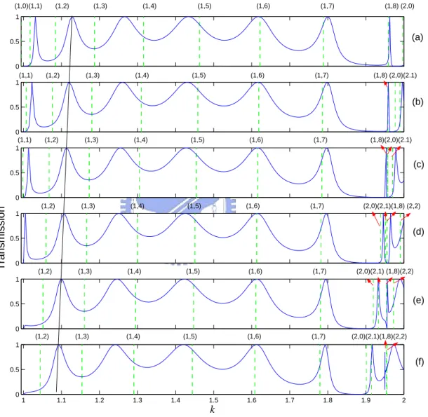
appear at the momentum after k =1.9 in Fig. 3.4(d). Before k =1.9 in Fig. 3.4(a)-(f), the profile just shift forward to low momentum. And the shift of profile just like the shift of the confined momentum of close ring (dashed line) before k =1.9 in Fig. 3.4(a)-(f). It is interesting to see if there is any significant difference before k =1.9 and after k =1.9 in Fig. 3.4. Consequently, we observe in Fig. 3.4 that the Fano structures appear near the confined state (1,8) of close ring in Fig. 3.4(d)-(f). And the different of Fig. 3.4(a)-(c) and (d)-(f) is that the confined state (1,8) is beyond the (2,0) in Fig. 3.4(d)-(f) but not in Fig. 3.4(a)-(e). And the Fano peak become shaper, when we vary the channel size from 1 to 0.95.
3.3
Approach to 1D rings
Here, we approach our result to 1D case and we just consider energy below the second subband and that particle propagates only within the first subband. In order to comparing more convenient, we use the longitudinal wave number k// =
p
E − E0
CR instead of the momentum k, where E is total energy and E0
CR is the energy at confined state (1,0) of close ring. And we define λ//= 2π/k//as the wavelength, and L1,2 = Rθ1,2 as armlengths,
here R = (r2+ r1)/2 and θ1,2 are the angles shown in Fig. 2.1. We compare the two cases
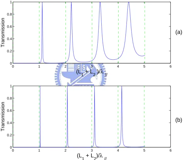
of broad channel (R/s = 3.5) and narrow channel (R/s = 9.5), where s is the width of ring. The transmission venues (L1 + L2)/λ// at symmetrical arms (L1 = L2) in the ring
CHAPTER 3. RESULT AND DISCUSSION OF OPEN QUANTUM RING WITHOUT MAGNETIC FIELD
0 0.5 1 0 0.5 1 0 0.5 1 0 0.5 1 Transmission 0 0.5 1 1 1.1 1.2 1.3 1.4 1.5 1.6 1.7 1.8 1.9 2 0 0.5 1 k (1,0)(1,1) (1,2) (1,3) (1,4) (1,5) (1,6) (1,7) (1,8) (2,0) (1,1) (1,2) (1,3) (1,4) (1,5) (1,6) (1,7) (1,8) (2,0)(2.1) (1,1) (1,2) (1,3) (1,4) (1,5) (1,6) (1,7) (1,8)(2,0)(2.1) (1,2) (1,3) (1,4) (1,5) (1,6) (1,7) (2,0)(2,1)(1,8) (2,2) (1,2) (1,3) (1,4) (1,5) (1,6) (1,7) (2,0)(2,1) (1,8)(2,2) (1,2) (1,3) (1,4) (1,5) (1,6) (1,7) (2,0)(2,1)(1,8)(2,2) (a) (b) (c) (d) (e) (f)
Figure 3.4: The solid line is transmission probabilities as functions of the electron mo-mentum of the OQR of r1 = 1, s = 1 and θ = π, for different r2 = 1(a), 0.99(b), 0.98(c),
CHAPTER 3. RESULT AND DISCUSSION OF OPEN QUANTUM RING WITHOUT MAGNETIC FIELD
0 1 2 3 4 5 6 0 0.2 0.4 0.6 0.8 1 (L 1 + L2 )/λ// Transmission 0 1 2 3 4 5 6 0 0.2 0.4 0.6 0.8 1 (L 1 + L2)/λ// Transmission (a) (b)
Figure 3.5: The solid line is transmission probabilities as functions of (L1 + L2)/λ// of the OQR of θ = π, for (a)R/s = 3.5, (b)R/s = 9.5
CHAPTER 3. RESULT AND DISCUSSION OF OPEN QUANTUM RING WITHOUT MAGNETIC FIELD
shift toward the left to be close to confined state of close ring , when the channel narrow down. And the confined states of close ring are dashed line in Fig. 3.5, and those dashed line are very close (L1+ L2)/λ = integer. It seems that the number of waves in the ring
is n when (L1+ L2)/λ = n.
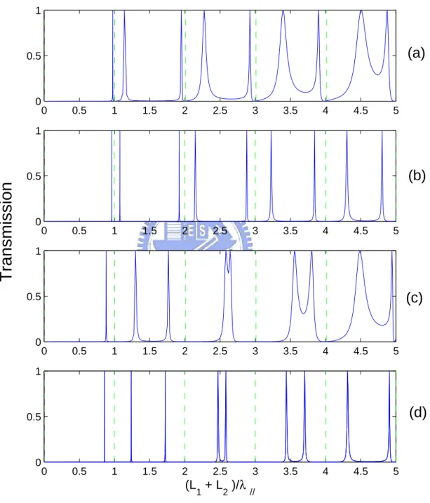
In section 3.2, we found that the Fano structure can be tuned by change geometry symmetric. Here, we would like to see the change of the Fano structure as approaching to 1D case. Fig. 3.6, shows the transmission probabilities for the case of asymmetrical arms. From Fig. 3.6, it is seen that the Fano structure become very sharp when the channel is narrower. But the Fano structures do not shift their position when the channel narrows down. This is different with the resonance peaks.
CHAPTER 3. RESULT AND DISCUSSION OF OPEN QUANTUM RING WITHOUT MAGNETIC FIELD
0 0.5 1 1.5 2 2.5 3 3.5 4 4.5 5 0 0.5 1 0 0.5 1 1.5 2 2.5 3 3.5 4 4.5 5 0 0.5 1 0 0.5 1 1.5 2 2.5 3 3.5 4 4.5 5 0 0.5 1
Transmission
0 0.5 1 1.5 2 2.5 3 3.5 4 4.5 5 0 0.5 1 (L 1 + L2 )/λ//(c)
(b)
(d)
(a)
Figure 3.6: The solid line is transmission probabilities as functions of (L1 + L2)/λ// of the OQR for (a)R/s = 3.5, L1/L2 = 0.9 (b)R/s = 9.5, L1/L2 = 0.9, (c)R/s = 3.5,
Chapter 4
Numerical results with finite
magnetic field
4.1
Magnetic field character on quantum transport
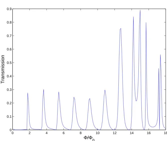
Figure 4.1 shown the transmission probability as a function of Φ/Φ0 for an AB ring,
the system parameters r2 = 2, r1 = 1, θ = π and k = 1.182, where Φ is flux through
the ring section area and Φ0 = h/2e is flux quantum. Form Fig. 4.1 we see that T
changes periodically with magnetic field, which is basic characteristic of the AB ring. The oscillating period is 2Φ0 = h/e. This is known as the (h/e) AB effect since one cycle
of oscillation corresponds to a change in the enclosed magnetic flux (Φ = BS),where S is the area of the ring. Moreever we can see that the peak of periodic oscillation may split into two peaks at Φ/Φ0 ≥ 16 see Fig. 4.1, then the periodic oscillation are disappearing
at large magnetic field.
4.2
Momentum characteristics on quantum transport
CHAPTER 4. NUMERICAL RESULTS WITH FINITE MAGNETIC FIELD 0 2 4 6 8 10 12 14 16 18 0 0.1 0.2 0.3 0.4 0.5 0.6 0.7 0.8 0.9
Φ
/
Φ
0Transmission
Figure 4.1: The transmission probability as a function of Φ/Φ0 for an AB ring, the
CHAPTER 4. NUMERICAL RESULTS WITH FINITE MAGNETIC FIELD
transmission of an OQR in weak and zero magnetic field, we can find that there are 14 peaks in weak magnetic filed and 7 peaks in zero field. It is shown that each peak has been splitted into two peaks when weak magnetic field is applied. And it can be also seen that there are Fano structure, locate at the bound states of a corresponding close ring.
For the case of low magnetic field, if we change the angle θ between the two leads of connected from the OQR, the transmission characteristics are shown in Fig. 4.3. From the Fig. 4.3, it is seen that the value of dip with transmission zero are increased by varying θ from π. However other shallow dips are decreased. Interestingly the Fig. 4.4 shows that the variation of transmission of OQR with high magnetic field, when we change θ. Then it show that those transmission in Fig. 4.4 only change a little as varying the angle θ. Hence, it seems that the interference effect are not obvious at large field.
CHAPTER 4. NUMERICAL RESULTS WITH FINITE MAGNETIC FIELD 1 1.1 1.2 1.3 1.4 1.5 1.6 1.7 1.8 1.9 2 0 0.1 0.2 0.3 0.4 0.5 0.6 0.7 0.8 0.9 1 k Transmission (1,1) (1,2) (1,3) (1,4) (1,5) (1,6) (1,7) (1,8)(2,0) (1,0)
Figure 4.2: The transmission of an OQR in weak magnetic field (Φ/Φ0 = 0.48, dash-dotted
CHAPTER 4. NUMERICAL RESULTS WITH FINITE MAGNETIC FIELD 1 1.1 1.2 1.3 1.4 1.5 1.6 1.7 1.8 1.9 2 0 0.1 0.2 0.3 0.4 0.5 0.6 0.7 0.8 0.9 1 k Transmission
Figure 4.3: The transmission of an OQR r2 = 2 and r1 = 1 in lower magnetic field
CHAPTER 4. NUMERICAL RESULTS WITH FINITE MAGNETIC FIELD 1 1.1 1.2 1.3 1.4 1.5 1.6 1.7 1.8 1.9 2 0 0.1 0.2 0.3 0.4 0.5 0.6 0.7 0.8 0.9 1 k Transmission
Figure 4.4: The transmission as a function of momentum k. The parameters are r2 = 2,
r1 = 1,and k = 1.182 in higher magnetic field (Φ/Φ0 = 9.87)for different θ = π(solid line),
Chapter 5
Numerical results with magnetic flux
5.1
Comparison with the 1D result
In this chapter, we show the result of an open quantum ring with a magnetic flux in center of ring. First, we compare our schemes with the 1D calculation in a chosen type of system. The way that we calculate the transmission probability for a 1D ring connected to two leads, which is the simplest multiply connected 1D system, using our connection schemes at the three-leg junction (Y junction) [23].
Fig. 5.1 shows the transmission probabilities obtained by different schemes. We have considered different flux Φ/Φ0 = 0 − 2.0, and in each case we have presented the result of
the 1D scheme with r = 3.5 and the results of the Q1D scheme with r2 = 4 and r1 = 3.
It is seen that in all cases, the difference between the Q1D and 1D results is slight in the scale of this graph. There are good comparisons between the results due to Q1D scheme and the 1D calculation.
5.2
Magnetic flux character on quantum transport
Fig. 5.2 presents the transmission probabilities of open quantum ring with r2 = 2, r1 = 1
CHAPTER 5. NUMERICAL RESULTS WITH MAGNETIC FLUX 0 1 2 3 4 5 6 0 0.5 0 0.5 0 0.5 0 0.5 0 0.5 0 0.5 0 0.5 0 (L 1+L2)/λ// Transmission (a) (b) (c) (d) (e) (f) (g)
Figure 5.1: The transmission probability T is plotted versus the dimensionless longitudi-nal wave number in Q1D scheme (r2 = 4, r1 = 3, solid line) and 1D(r = 3.5, dash line)
CHAPTER 5. NUMERICAL RESULTS WITH MAGNETIC FLUX
Fig. 5.2, the oscillating period is Φ/Φ0 = 2(Φ0 = h/2e). Moreover, there are two kinds of
strange dips. One is the value of dip equals zero and another is that the minimum value of dip is form of envelope.
Then we choose some dips and peaks, and plot wave function probability at the max-imum value of peak and the minmax-imum vale of dip. They are shown in Fig. 5.3. For peaks, the wave function at Φ/Φ0 = (a)12.93 and (c)14.97 are seem that electron like to exit from
lower branch and stay on upper branch. On the contrary, the wave function at Φ/Φ0 =
(b)13.21 and (d)15.21 seem that like to exit from upper branch and stay on lower branch. For dips, the wave function probability at upper and lower branch for Φ/Φ0 = (e)15.09
and (f)14.1 are symmetry. It differs from the wave function at peaks.
−200 −15 −10 −5 0 5 10 15 20 0.1 0.2 0.3 0.4 0.5 0.6 0.7 0.8 0.9 1 Φ/Φ 0 Transmission
Figure 5.2: The transmission probability as a function of Φ/Φ0 for an OQR with a
CHAPTER 5. NUMERICAL RESULTS WITH MAGNETIC FLUX −2 −1 0 1 2 −2 −1 0 1 2 x y −2 −1 0 1 2 −2 −1 0 1 2 x y −2 −1 0 1 2 −2 −1 0 1 2 x y −2 −1 0 1 2 −2 −1 0 1 2 x y −2 −1 0 1 2 −2 −1 0 1 2 x y −2 −1 0 1 2 −2 −1 0 1 2 x y (b) (a) (c) (d) (e) (f)
Figure 5.3: The wave function of Φ/Φ0= (a)12.93, (b)13.21, (c)14.97, (d)15.21, (e)15.09,
Chapter 6
Conclusions and future work
Throughout the thesis, the quantum transport properties through a OQR are calculated and numerically analyzed. We have found that the resonant peaks correspond to the bond states of a close ring. Moreover, we can tune the Fano structure from broad to sharp by varying the symmetry of OQR and turn the Fano structure from sharp to broad by widening the channel width of the ring. Then approaching to 1D case, the resonance peaks become shaper and shift toward the left to be close to bound of close ring, when the channel narrow down. We have found that the AB effect when the external field are applied in the ring and the oscillating period Tp = 2Φ0 = h/e. It should be noted that
the periodic oscillations are disappear at high magnetic field. If we change the angle θ of two lead for low and high magnetic field, we can found that it is sensitive to changing angle θ for small magnetic field but not for large magnetic field. In the thesis, a number of interesting phenomena on quantum transport through an OQR are observed. For the case of zero magnetic field, we have found that the transmission resonances a function of energy has only one missing to match with the bound-state levels of a close ring. The physics behind is still not very clear, and our group member will make diligence on the detail transport mechanisms through the OQR systems. Further studies such as spin-orbit interaction, and time-dependent modulation will be studied in the near future.
Bibliography
[1] A. Lorke, R. J. Luyken, A. O. Govorov, J. P. Kotthaus, J. M. Garcia,and P. M. Petroff, Phys. Rev. Lett. 84, 2223 (2000).
[2] J. M. Garcia, G. Medeiros-Ribeiro, K. Schmidt, T. Ngo, J. L. Feng,A. Lorke, J. Kotthaus, and P.M. Petroff, Appl. Phys. Lett. 71, 2014 (1997).
[3] R. J. Warburton et al., Nature 405, 926 (2000). A. Lorke et al., Phys. Rev. Lett. 84, 2223 (2001).
[4] M. Buttiker, Y. Imry, and R. Landauer, Phys. Lett. A 96, 365 (1983); M. Buttiker, Y. Imry, and M. Ya. Azbel, Phys. Rev. A 30, 1982 (1984); M. Buttiker, in SQUID’
85-Superconducting Quantum Interference Devices and Their Applications, Ed. by
H. D. Haklbohm and H. Lubbig (Walter de Gruyter, New York, 1985).
[5] R. A. Webb, S. Washburn, C. P. Umbach, and R. B. Leibowitz, Phys. Rev. Lett. 54, 2696 (1985).
[6] Y. Aharonov and D. Bohm, Phys. Rev. 115, 485 (1959)
[7] A.G. Aronov and Y.V. Sharvin, Rev.Mod. Phys. 59, 755 (1987).
[8] Timp G., Chang A. M., Cunningham J. E., Chang T. Y., Mankiewich P., Behringer R. and Howard R. E., Phys. Rev. Lett., 58 (1987) 2814.
[9] Fuhrer A., L¨uscher S., Ihn T., Heinzel T., Ensslin K., Wegscheider W. and Bichler
BIBLIOGRAPHY
[10] Pedersen S., Hansen A. E., Kristensen A., Sorensen C. B. and Lindelof P. E., Phys. Rev. B, 61 (2000) 5457.
[11] U. Fano, Phys. Rev. 124, 1866 (1961).
[12] R. K. Adair, C.K. Bockelman, and R. E. Peterson, Phys. Rev. 76, 308 (1949). [13] U. Fano and A. R. P. Rau, in Atomic Collisions and Spectra (Academic Press, Orland,
1986).
[14] F. Cerdeira, T. A. Fjeldly, and M. Cardona, Phys. Rev. B 8, 4734 (1973).
[15] J. Faist, F. Capasso, C. Sirtori, K.W. West, and L. N. Pfeiffer, Nature (London) 390, 589 (1997).
[16] G. D. Mahan, Many-Particle Physics (Plenum Press, New York, 1990).
[17] V. Madhavan, W. Chen, T. Jamneala, M. F. Crommie, and N. S. Wingreen, Science 280, 567 (1998).
[18] J. Li, W. D. Schneider, R. Berndt, and B. Delley, Phys. Rev. Lett. 80, 2893 (1998). [19] J. G¨ores et al., Phys. Rev. B 62, 2188 (2000).
[20] J. Imry, in Directions in Condensed Matter Physics, edited by G. Grinstein and G. Mazenko (Wold Scientific, Singapore, 1986), p. 101; C. W. J. Beenakker and H. Van Houten, Solid State Phys. 44, 1 (1991); S. Datta, Electronic Transport in Mesoscopic
Systems (Cambridge University Press, Cambridge, England, 1995).
[21] R. A. Webb, S. Washburn, C. P. Umbach, and R. B. Laibowitz, ”Observation of h/e aharonov-bohm oscillations in normal-metal rings”, Phys. Rev. Lett. 54, 2696?699 (1985).
[22] V. Chandrasekhar, M. J. Rooks, S. Wind, and D. E. Prober, ”Observation of aharonov-bohm electron interference eoeects with periods h/e and h/2e in individual
BIBLIOGRAPHY
[23] K. K. Voo, S. C. Chen, C. S. Tang, and C. S. Chu, Phys. Rev. B 73, 035307 (2006). [24] The 1D data is due to K.-K. Voo (unpublished).
![Figure 1.2: Transmission-electron micrograph of ring-shaped conductor [6]. The inside diameter of loop is 784 nm and the width of the wires is 41 nm (adapted from Ref.6).)](https://thumb-ap.123doks.com/thumbv2/9libinfo/8749429.205582/15.892.324.620.219.403/figure-transmission-electron-micrograph-conductor-inside-diameter-adapted.webp)