違約風險對權益流動性之影響--高財務危機成本時期之分析

全文

(1)୮ Ҥ ҫ ೮ δ Ꮱ! !. !. !. !. !. ૲଻޼ᑪ‫!ۺ‬ ᅺ!γ!ፕ!Ў!. 違約風險對權益流動性之影響 --高財務危機成本時期之分析. The Effect of Default Risk on Equity Liquidity When Expected Financial Distress Costs are High. 研究生：陳禹丹指導教授：鍾惠民許和鈞. 副教授教授. ύ!๮!҇!୯!ΐ!˺!Ѥ!ԃ!Ϥ!Д!.

(2) 違約風險對權益流動性之影響 --高財務危機成本時期之分析 The Effect of Default Risk on Equity Liquidity When Expected Financial Distress Costs are High 研究生：陳禹丹. Student：Yu-Dan Chen. 指導教授：鍾惠民博士. Advisor：Dr. Huimin Chung. 許和鈞博士. Dr. Her-Jiun Sheu. 國立交通大學財務金融所碩士論文 A Thesis Submitted to Graduate Institute of Finance College of Management National Chiao Tung University in partial Fulfillment of the Requirements for the Degree of Master of Science in Finance June 2005 Hsinchu, Taiwan, Republic of China. 中華民國九十四年六月.

(3) 違約風險對權益流動性之影響 --高財務危機成本時期之分析. 研究生：陳禹丹. 指導教授：鍾惠民許和鈞. 副教授教授. 摘要. 本文旨在探討違約風險與權益流動性之關係。過去文獻指出財務狀況險惡的公司常會吸引資訊優勢交易者進入市場交易該股，而無資訊優勢的一般流動性需求交易者則退出市場，實務上，公司違約可能性通常會被經理人隱匿而造成市場上資訊不對稱成本提高，此代理成本使得承擔較高風險的造市者會利用增加價差以保證其利潤。本文利用 Merton’s Model(1974)來估計公司違約機率，並研究是否高財務危機公司其股票交易買賣價差較高。再者，使用追蹤資料門檻迴歸模型來探討違約風險與流動性之間的非線性關係。實證結果顯示，第一，違約風險對於流動性有顯著地正向影響；第二，兩變數存在非線性關係；最後，比起一般時期，當市場處在公司醜聞爆發時期，上述兩項關係亦特別明顯存在，使得交易成本上昇及交易萎縮，因而加速體質不良公司倒閉或股價重挫，亦即地雷股爆發會有群聚現象之因，財務不佳之公司會遭受較差的流動性，是故，除了直接或間接財務危機成本，流動性成本也可歸諸於公司財務危機成本之一。. 關鍵詞：違約風險、權益流動性、財務危機成本、追蹤資料模型、門檻迴歸模型. i.

(4) The Effect of Default Risk on Equity Liquidity When Expected Financial Distress Costs are High Student：Yu-Dan Chen. Advisor：Dr. Huimin Chung Dr. Her-Jiun Sheu. Graduate Institute of Finance College of Management National Chiao Tung University. ABSTRACT. This dissertation is to demonstrate the relation between default risk and equity liquidity. Market makers will widen spreads if the trading proportion of informed traders increases and uninformed traders exit market as firm’s financial performance deteriorates. Increased default probability usually concealed by managers will enlarge asymmetric information costs and thus market makers offer greater bid-ask spreads to protect their profit. Default risk measured by Merton’s option pricing model to investigate whether firms with financial distress possess higher bid-ask spreads. Furthermore, we take the panel threshold regression model to examine the possible non-linear relationship between default risk and equity liquidity. The result shows default risk observably has more significant and stronger relation to equity liquidity in the corporate scandal disaster period than usual time. We infer that results in corporate scandal and listed company bankruptcy events always lead to a chain reaction. The happenings of firm’s bankrupt and enormous dump of prices are generally clustered, in particular for the firms with deteriorating financial condition.. Keywords: Default Risk, Equity Liquidity, Financial Distress Costs, Panel Data, Threshold Regression ii.

(5) Acknowledge. 常常覺得到交大就讀財金所實在是上天冥冥中的安排，首先要謝謝貼心安排讓我住宿一晚以順利赴考的表哥俊穎，才有幸來到交大拜在鍾惠民老師與許和鈞老師門下，感謝兩位老師給我機會並盡力指導。也因此才有緣認識這群好友--而音學姊、偉立、小明、智琦、阿德、筱芳、婉儀、冠宇、 Dora，有了大家的互助，在課業與工作方面我才有所進步與發揮，有了大家的陪伴，在沮喪挫敗時才能走過低潮疲乏。短短七百多個日子卻在我的人生中寫下最多奇妙的故事，謝謝牛牛經常開導我，謝謝幸運之神紅豆只要一出現程式總能突破瓶頸。謝謝老天眷顧我，我是個幸運兒，能擁有朋友的支持與鼓勵，最珍貴的是有個平凡而幸福溫暖的家，謹將本論文獻給總是對我無私付出的爸爸媽媽及弟弟妹妹，願大家身體健康平安快樂。. 禹丹. iii. 2005.6.

(6) CONTENTS. Chinese Abstract i English Abstract ii Acknowledge. iii. Table of Contents List of Tables. iv. v. 1. Introduction..............................................................................................................1 2. Literature review......................................................................................................5 2.1 Market liquidity and bid-ask spread............................................................5 2.2 Proxies for the firm’s financial distress........................................................6 3. Data and Methodology ..........................................................................................10 3.1 Data ...............................................................................................................10 3.2 Methodology ................................................................................................. 11 4. Empirical tests and results ....................................................................................22 4.1 Sample characteristics .................................................................................22 4.2 Results of cross-sectional regression...........................................................22 4.3 Results of panel data regression .................................................................23 4.4 Results of panel data threshold regression ................................................24 5. Conclusion ..............................................................................................................26 REFERENCES...........................................................................................................28 Appendix.....................................................................................................................37. iv.

(7) List of Tables. TABLE 1 Descriptive statistics of selected variable ...............................31 TABLE 2 Pearson correlations coefficients of selected variable ....31 TABLE 3 Cross-sectional regression results ...............................................32 TABLE 4 Cross-sectional regression results (key regressor: DLI)..............................................................................33 TABLE 5 Results of panel data regression model (key regressor: PDLI)...........................................................................34 TABLE 6 Results of single threshold model (key regressor: PDLI)...........................................................................35 TABLE 7 Results of double threshold model only for Period 2 (key regressor: PDLI)...........................................................................36. v.

(8) 1. Introduction. A lot of researches have studied the costs of financial distress, including direct costs and indirect costs1. Nevertheless, except for direct costs and indirect costs, recently new notion of financial distress costs is proved. Bagehot (1971), Copeland and Galai (1983), Glosten and Milgrom (1985), and Kyle (1985) argue the existence of informed trades is the reason that causes the stock liquidity to be worse when performance of a company weakens and probability of financial distress increases. Using alternative proxies2 of the firm’s financial distress Agrawal, et al., (2004) demonstrates that firms with financial distress suffer for reduced stock liquidity by increasing bid-ask spread. Odders-White and Ready (2004) confirms adverse selection costs are greater as debt rating are poorer but bond rating is slow with a lag to react asset value uncertainty. The measures of financial conditions or credit risk employed in Odders-White and Ready (2004) and Agrawal, et al., (2004) lack of predictive content of their measures of the financial strength of companies. Vassalou and Xing (2004) use Merton’s option pricing model to compute default measures for individual firms and access the effect of default risk on equity returns. Bid-ask spread, one of the measures of stock liquidity, contains three kinds of costs: (1) order processing costs, (2) inventory holding costs and (3) adverse information costs. If investors trade on the basis of superior information, adverse information costs increase to compensate market maker for losses to informed traders. Market makers set the spreads wide enough to guarantee that their profits in trades to uninformed traders will cover the expected losses from the trades with 1. The direct costs comprise legal and administrative expenses of bankruptcy proceedings (Warner, 1977; Weiss,1990); the indirect costs consist of management resources devoted to resolving financial distress, loss of suppliers and customers, and constraints on the firm’s financing and investment opportunities (Altman,1984;Titman,1984;Wruck,1990). 2 Those proxies of the firm’s financial distress include Tobin Q, S&P bond rating, accounting measure of financial performance and S&P common stock ranking. 1.

(9) informed traders. Moreover, trading in the firm’s security may be increasingly dominated by informed investors when performance and financial condition of a firm are terrible. Thus the larger the proportion of informed traders in a given stock, the wider the bid-ask spread. Consequently, the existence of informed trades is the reason that causes the stock liquidity to be worse when performance of a company weakens and probability of financial distress increases. The measures of financial conditions or credit risk employed in Agrawal, et al., (2004) and Odders-White and Ready (2004) do not consider the information content of market’s perception of default likelihood. Using the default likelihood measure calculated by Merton’s method, this paper investigates whether financially ailing firms do indeed have higher bid-ask spreads. Furthermore, in the period of expected high financial distress costs, does default risk observably affect stock liquidity more than usual time? What does the period of expected high financial distress costs mean on earth? In this paper, the stock market to which traders are lacking confidence and become over-pessimistic is described as the period of expected high financial distress costs. During the period of the fourth quarter in 2001, most of the global finance markets are sluggish, especially the stock market of American, owing to explosion of a series of corporate scandals. The bankruptcy of Enron Corp3, the biggest corporate bankruptcy in U.S. history, is infectious. Investors were more and more sensitive to financial statement and credit risk of company. From what we have mentioned above, in this research it is the period of high financial distress costs that the eight months from October 2001 to May 2002 is regarded as. Hence, the purpose of this paper is to demonstrate whether default risk 3. On December 2, 2001, the energy giant “Enron Corp.” announced that it and 14 of its subsidiaries have filed voluntary petitions for Chapter 11 reorganizations with the U.S. Bankruptcy Court for the Southern District of New York. Enron listed $49.8 billion in assets and $31.2 billion in debts. 2.

(10) observably has stronger correlation with equity liquidity during the Enron crisis period than usual time. We infer that the corporate scandal of Enron and some listed company bankruptcy events are the source of that investors become over-pessimistic and reduce trading in equity market, especially those stocks in poor financial condition. What is more, to account for the potential non-linear relationship between default risk and equity liquidity, we make an effort to estimate and test threshold effect. The percentage bid-ask spread will be used to measure the cost of equity liquidity and Merton’s (1974) option pricing model is applied to estimate default risk for individual firms. The default risk measure is called as “Default Likelihood Indicator (DLI)”. The panel data regression and econometric techniques developed in Hansen (1999) appropriate for threshold regression with panel data are applied here in order to investigate the distinction effect between high default risk group and low one on liquidity. Our empirical result reaches a conclusion concerning the influence of default risk on stock liquidity and whether the results are any more significant in the period with high financial distress costs. First of all, the finding shows the perceived default risk at the beginning of the month has predictive contents on the liquidity (average bid-ask spread) of the month. DLI reveals an extremely significant positive relation to percentage bid-ask spread, proving default risk is one of the key determinants of liquidity cost and firms with trouble financial condition suffer from the cost of reduced liquidity. It is more interesting that especially during the period with expected high financial distress costs, the increasing credit risk of poorly financial condition firms will indeed contribute to the percentage bid-ask spread to raise more than usual period. Moreover, dissimilar classes of credit risk partition according to the estimated thresholds are able to manipulate the liquidity cost in enormously diverse weights. 3.

(11) We posit that firms bankrupt or stock prices dump in clustered time, particularly for those stocks with high default risk, is derived from the relation between default risk and equity liquidity becomes stronger when the financial distress costs are severe. This is to say, during the period of high financial distress costs, market makers have stronger motivation to magnify spreads in response to the potentially increased probability of trades against informed investors. And then the worse equity liquidity is able to precipitates default of poor performance firms. The remainder of this paper is organized as follows. The next section introduces the review of related literature. Section 3 discusses data and methodologies, such as default likelihood indicators, panel data regression model and threshold regression model. Empirical tests and results are undertaken in section 4. Section 5 outlines conclusion.. 4.

(12) 2. Literature review. 2.1 Market liquidity and bid-ask spread. Market markers play an important role in facilitating trades by providing stock liquidity in some stock exchanges. The notion of liquidity refers to the ability of a trader to execute a trade or liquidate a position quickly, anonymously with little or no cost, risk or inconvenience. Market liquidity measures the cost of taking ownership positions in firm’s equity like the notion of marketability. A stock with lower liquidity cost is always close to possess excellent marketability that benefit greatly to investors allocating their ownership positions. However even the big standardized markets are not perfectly liquid. The main source of liquidity costs is the bid-ask spread. The quoted bid-ask spread is the difference between the ask price quoted by a trader and the bid price quoted by a trader at a point in time. Following Demsetz (1968), we can think of specialists as providing the service of immediate trading and bid-ask spreads cover the costs of market maker providing quick exchange. The literature of Stoll (1978) points out that the quoted bid-ask spread contains three costs faced a dealer: (1) order processing costs, the costs of settling trades, recording and clearing a transaction; (2) inventory holding costs, the price risk and opportunity cost of holding securities; and (3) adverse information costs which increase if investors trade on the basis of superior information. In the early literature such as Demsetz (1968) and Tinic (1972), order processing costs receives greater emphasis, but all researches on the bid-ask spread recognize the importance of these costs. Stoll (1978) and Ho and Stoll (1981) find evidence that inventory holding costs arise from the risk assumed by a dealer, and Amihud 5.

(13) and Mendelson (1980) model the effect of constraints on inventory size. Recent academic studies have emphasized the importance of adverse information costs (e.g., Bagehot(1971), Copeland and Galai (1983), Glosten and Milgrom (1985), Kyle (1985) and Easley and O’Hara (1987)). Those papers model the equilibrium spreads in the presence of informed traders. Market makers trade against two sorts of investors, informed traders and uninformed traders4. Generally if some traders hold superior information, then the market maker loses on average to those traders. As a result the market maker will want to profit in their transactions with noise traders obtaining no private information by setting the spreads wide enough to guarantee that their profits in trades to uninformed traders will cover the expected losses from the trades with informed traders. However, when operating performance and financial condition of a firm are terrible, trading in the firm’s security may be increasingly dominated by informed investors. Thus the larger the proportion of informed traders in a given stock, the wider the bid-ask spread.. 2.2 Proxies for the firm’s financial distress. Many famous studies assert a series of proxies for the firm’s financial distress, such as Tobin’s Q, default probability, common stock ranking and accounting measure. Several papers (e.g., Brook and Rao, 1994; Gilson, 1989; Lang et al., 1989; Lindenberg and Ross, 1981) adopt Tobin’s Q as a measure of firm’s financial condition. Tobin’s Q is defined as [(market value of equity + book value of debt)/book value of total assets]. The lower the ratio of Tobin’s Q, the worse the firm’s performance. 4. Those possess private information and fail to reflected in the prices at the time of the trade are called informed traders. On the other hand, uninformed traders are who trade for reasons like liquidity demand, risk aversion, and possibly random speculation. 6.

(14) Several early literatures employ accounting items as a measure of firm’s financial distress. DeAngelo & DeAngelo (1990) verifies three groups of companies, high performance firms, medium performance firms and low performance firms, by income and pre-tax operating income. High performance firms are defined as having five years of positive income and pre-tax operating income. Firms with three years of negative income or negative pre-tax operating income during the five years proceeding the proxy year are defined as firms with low performance. Firms that do not fall in either category are classified as medium performance firms. As for bond rating, this indicator is produced as measure of the firm’s default risk by credit rating companies. Agrawal, et al., (2004) and Odders-White and Ready (2004) use bond rating as a proxy for the firm’s default risk which contains a wide array of factors, such as the firm’s market value, collateral value of its assets, indenture provisions, existence of third party guarantees of debt service, potential third party insurance of timely debt service, leased assets, cash flows from segregated or trusted assets, security rights in assets. Thus bond rating fails to be recognized by any single accounting measure of default risk. Odders-White and Ready (2004) present a theoretical model that illustrates the potential linkage between a firm’s bond rating and the level of adverse selection in the trading of the firm’s equity. Also it suggests ways to decompose the standard adverse selection measures to better isolate the uncertainty parameters related to credit ratings. In their model, the value of a firm’s assets changes in response to both publicly observed and privately observed shocks. The paper concludes that bond ratings are able to capture more information than easily accounting variables and ratings changes can be predicted using current levels of adverse selection, which suggests that credit rating agencies fail to respond new information without delay. Moreover, Vassalou and Xing (2004) is the first research that uses Merton’s model to calculate default 7.

(15) probability for individual firms. They call the default risk measure as Default Likelihood Indicator (DLI)5. The finding asserts stocks with both of higher default risk and smaller size or higher book-to-market ratio possess greater equity return. Agrawal, et al., (2004) also use common stock ranking as a proxy for financial condition. Obviously the common stock ranking is excellent than any single accounting measure because the ranking consists of many kinds of accounting items. For example, the S&P Common Stock Ranking is another measure of historical performance and is an appraisal of past performance of a stock’s earnings and dividends and the stock’s relative standing as of a company’s current fiscal quarter end6. Growth and stability of earning and dividend are the most important factors in scoring S&P’s earnings and dividends rankings for common stocks. Pay careful attention to previous studies has used either accounting measure or bond market information as the proxy for financial condition. There are some defects using accounting items to measure the firm’s financial distress. First, the accounting information is backward looking because financial statement aim to report a firm’s past performance, rather than its future scenario. Besides, another defect, the most important one, is that accounting models do not think about the volatility of a firm’s assets. Accounting models involve that the firms with similar financial ratios will be in the same financial condition. In contrast, default likelihood indicator uses the market value of a firm’s equity to estimates its market value and volatility of a firm’s assets and calculate its default risk. Rather than using the book value of equity or assets, as the accounting models do. Furthermore, default likelihood indicator takes into account the volatility of a firm’s assets to obtain new information. The probability of default risk varies with. 5 6. The detail content of DLI is introduced in section 3.2.1(page 11). Source: Compustat Manual, Section 8-B, page 27. 8.

(16) different volatility of a firm’s assets. In other words, the volatility of a firm’s assets provides key information about the firm’s default risk.. 9.

(17) 3. Data and Methodology. 3.1 Data. The component stocks of S&P500 traded on the New York Stock Exchange (NYSE) are elected to be our empirical sample to investigate if firm’s financial condition can explain equity liquidity. Stoll (2000) concludes that market structure has a clearly effect on bid-ask spreads. Spreads continue to be larger significantly on the Nasdaq dealer market than on the NYSE/AMSE auction market. To eliminate the deviation between various markets, we only use the component stocks of S&P500 listed in NYSE. Thus, the number of observant firm is decrease to 423 firms in our sample. Moreover, the period of our experimental research is from February7 1, 2001 to May 30, 2002. The firms that have at least one missing value of variable used in this study are deleted from our sample. Consequently, our sample size reduces to 276 firms and the number of observations is 4416. In our cross-sectional model, the depended variable is percentage bid-ask spread (PSP) and explanatory variables are close price (CP), the number of trade (NT), volatility (SIG), market value (MV) and Default Likelihood Indicators (DLI). PSP is calculated as the average of readings in final 60 seconds of ($Spread/Price)×100 each trading day. CP means the closing price every trading day. NT represents the number of trades per day. And finally each firm gets the average of daily data like PSP, CP and NT for the entire month. We compute the standard deviation of daily stock returns for a given month as the volatility of these daily returns over that 1-month period (SIG). MV is stock’s monthly market value. The book value of total. 7. NYSE switched to the decimal pricing system on January 29, 2001. Thus the period of our research starts from February 1,2001. 10.

(18) debt includes both current and long-term. DLI are nonlinear functions of the default probabilities of the individual firms. We estimate DLI by using the contingent claims methodology of Black and Scholes (1973) and Merton (1974). In order to calculate the proxy of equity liquidity, percentage bid-ask spreads, and other variables used in our cross-sectional model, daily intraday trade and quoted data for the 423 stocks are taken from the data file compiled by the Trade and Quoted (TAQ). We use the COMPUSTAT annul file to get “Market value”, “Debt in One Year” , “Long-Term Debt ” and “Total liabilities” series for all companies8. We acquire information on daily stock returns from the Center for Research in Securities Prices (CRSP) daily return files9. To calculate DLI, we observe monthly 1-year T-bill rate d from website of The Federal Reserve.. 3.2 Methodology. 3.2.1 Proxy for the firm’s financial condition: Default Likelihood Indicators. Vassalou and Xing (2004) is the first research of using Merton’s model to calculate default measures for individual firms and appraise the effect of default risk on equity returns. The conception of Merton (1974) is that the equity of a firm is thought of as a call option on the firm’s assets and then one can estimate the value of equity by using Black and Scholes (1973) formula. Our procedure in calculating default risk measures using Merton’s option pricing model is similar to the one used by KMV. 8. Because little information for 423 firms is not obtained on COMPUSTAT we lose a small number of stocks each month when merging the TAQ database with the variables calculated from COMPUSTAT. 9 Because little information for 423 firms is not obtained on CRSP we lose a small number of stocks each month when merging the TAQ database with the variables calculated from CRSP. 11.

(19) We assume the capital structure of the firm including equity and debt. The market value of a firm’s underlying assets follows a Geometric Brownian Motion (GBM) of the form:. dVA = µVAdt + σ AVAdW. Where VA is the firm’s value with an instantaneous drift µ. (1). and an. instantaneous volatility σ A . A standard Wiener process is W . Let X t be the book value of the debt at the time t, that has maturity equal to T. X t is used as the strike price of a option, since the market value of equity, VE , can be regard as a call option on VA with time to expiration equal to T. By the Black and Scholes model for call options, the market value of equity will be estimated: V E = V A N ( d 1 ) − Xe − rT N ( d 2 ). (2). where. d1 =. ln( V A / X ) + ( r +. σA T. 1 2 σ A )T 2 , d 2 = d1 − σ A T. (3). r is the risk-free rate, and N (．) is the cumulative density function of the standard normal distribution. An iterative procedure is adopted to estimate σ A and then to estimate daily value of VA for each sample month. As follow steps: Step1). Daily data from the past 12 months will be using to secure an estimate of the volatility of equity σ E , which is then viewed as an initial value for the estimation of σ A , σˆ A (1) .. Step2) Using the Black and Scholes formula Eq.(2), we obtain VA using VE as the market value of equity of that day for each trading day of the past 12. 12.

(20) months. In this mode, we capture daily values of VA for the past 12 months. Step3). We then compute the standard deviation of those VA from the last step, which is used as the value of σ A , σˆ A ( 2) , for the next iteration.. Step4). Step2) to Step3) are repeated to obtain σˆ A (3), σˆ A (4) ,…et al., until the values of σ A from two consecutive iterations converge. Our tolerance level for convergence is 10E-4.. Step5). Once the converged value of σ A is obtained, we use it to back out daily values of VA for month t through Eq.(2).. The above procedure is repeated at the end of every month, resulting in the estimation of monthly values of σ A . The estimation window is always kept equal to 12-months. The risk-free rate used for each monthly iterative process is the 1-year T-bill rate observed at the end of the month. Once daily values of VA for month t are estimated, we can compute the drift µ, by calculating the annual compound return rate of asset value, log(V A, t −1 / V A, t − q ) . The default measure is the probability that the market value of firm’s assets will be less than the book value of the firm’s liabilities as maturity T10. In other words,. Pdef. ,t. = Pr( V A ,t + T ≤ X t V A ,t ) = Pr(ln( V A ,t + T ) ≤ ln( X t ) V A , t ). (4). Because the value of the assets follows the GBM of Eq.(1), the value of the assets at any time t is given by:. 10. We use the “Debt in One Year” plus the half of “Long-Term Debt” as book value of debt. 13.

(21) ln( V A ,t + T ) = ln( V A ,t ) + ( µ −. ε t+T =. σ A2 2. ) T + σ A T ε t+T ,. (5). W (t + T ) − W (t ) , and ε t + T ~ N ( 0 ,1) T. (6). Hence, we can get the default probability as follows:. ⎞ ⎛ σ2 Pdef ,t = Pr ⎜⎜ ln( V A ,t ) − ln( X A ,t ) + ( µ − A ) T + σ A T ε t + T ≤ 0 ⎟⎟ 2 ⎝ ⎠ 2 V ⎞ ⎛ σ ⎟ ⎜ ln( A ,t ) + ( µ − A ) T Xt 2 ⎜ (7) Pdef ,t = Pr − ≥ ε t+T ⎟ ⎟ ⎜ σA T ⎟ ⎜ ⎠ ⎝ Distance to default (DD) could be defined as follows:. [. DD t = ln( V A ,t X t ) + ( µ − 12 σ A2 )T. ]. σA T. (8). When the ratio of the value of assets to debt is less than 1 or its log is negative, default occurs. The DD tells us by how many standard deviations the log of this ratio needs to deviate from its mean in order for default to occur. Pay careful attention to although the value of the call option in Eq.(2) does not depend on µ, DD does, resulting from DD depends on the future value of assets which is given in Eq.(3). Using the normal distribution implied by Merton’s model, the theoretical 11 probability of default, called Default Likelihood Indicators (DLI), will be given by:. P def = N ( − DD ) = N ( −. ln(. V. A ,t. X. t. ) + (µ −. σ. 11. A. T. 1 2. σ. 2 A. )T. ). Strictly speaking, Pdef is not a default probability because it does not correspond to the true probability of default in large samples. Thus Vassalou and Xing (2004) do not call that measure default probability, but rather DLI. 14. (9 ).

(22) DLI increases as (1) the value of debt raises, (2) the market value of equity as well as assets goes down, and (3) the assets volatility increases. Comparatively, DLI is superior to other approaches using accounting financial information to measure default risk. DLI has a range of strengths as follows: (1) it has strong theoretical underpinnings; (2) default likelihood indicator takes into account the volatility of a firm’s assets; (3) it is forward looking based on stock market data rather than historic book value accounting data.. 3.2.2 Regressions with control variables. The important factors of effect percentage bid-ask spreads have been approved by numerous earlier papers (e.g. Benston and Hagerman (1974), Tinic and West (1972) and Stoll (1978)). Besides stock price, the spread is influenced by some factors such as trading volume, variance of stock returns, market value of equity, and even the structure of exchange market. The declining prices of poorly performing firms will make percentage bid-ask spreads to rise. In particular, volatility of stock returns, which proxies for informed trading (Black, 1986), may rise and increase in spreads. It is also possible that although trading by informed investors rises, trading volume in general will decline because of fewer investors in the market, hence higher spreads ensued. For the purpose of examining the influence of the firm’s default risk on the bid-ask spreads clearly, we recommend controlling for these determinants. Under controlling variables in our regressions and find that the increase in spreads is still directly linked to the firm’s financial condition. Every variable is monthly average data except for DLI. DLI is default probability of the first trading day for each month. That implies that DLI forecasts PSP in ex ante base. Following most of the literature, we employ log regression. Consequently, our 15.

(23) cross-sectional regression has the following form:. PSPit = a + b1 logCPit + b2 logNTit + b3 SIGit + b4 logMVit + b5 DLIit + ε it. (10). Based on the results of past literature, we suppose b1, b2 and b4 should be negative, and b3 be positive. Because higher default risk implies financial condition exacerbation, b5 should be predictable positive according to Agrawal, et al., (2004). Considering the heteroscedasticity of data, we use generalized least squares estimation (GLS) to estimate the coefficients of these explanatory variables in Eq. (10) and test statistical significance.. 3.2.3 Panel data models. The important motivation for using panel data is to solve the omitted variables problem. If the omitted variable is correlated with explanatory variables, we cannot consistently estimate parameters without additional information. It is uncertain whether the explanatory variable, DLI, is exogenous. If the test result shows that an omitted variable is presence, unobserved effects panel data model is one of ways to address the problem. First of all, suppose that the omitted variable is not change over time. That means the omitted variable has the same effect on the mean response in each time period. An unobserved, time-constant variable is called an unobserved effect in panel data analysis. Moreover there are two different estimation methods, including random effects estimation and fixed effects estimation which be adopted in this. 16.

(24) study. In modern econometric parlance, differing from traditional notion12 to panel data models, “random effect” is synonymous with zero correlation between the observed explanatory variables and the unobserved effect. However, “fixed effect” means that one is allowing for arbitrary correlation between the observed explanatory variables and the unobserved effect. The random effects approach estimates the coefficients under the assumption that the unobserved effect is orthogonal to explanatory variables. But this assumption is too strong to satisfy easily. On the other hand, fixed effects approach releases the strict exogeneity in addition to orthogonality between the observed explanatory variables and the unobserved effect in random effects approach. Thus fixed effects approach will more make sense for our nonexperimental panel data. More detailed discussion concerning fixed effects methods are as follows. The linear unobserved effects model for T time periods will be written as:. y it = x it β + c i + u it. (11). where the subscript i is cross section observation indexing individuals such as firms and subscript t indexes time. x it is 1 × k and can comprise observable variables that change across t as well as i, variables that change across t but not i, and variables that change across i but not t. ci presents unobserved effects that change across i but not t, thus also named individual effect. As what we have mentioned, the individual effect ci be viewed as correlation with the x it in fixed effect models. The uit called idiosyncratic errors or idiosyncratic disturbances change across not only t but also i. 12. In the traditional approach, “random effect” means unobserved component is treated as a random variable. In contrast, an unobserved component is treated as parameter to be estimated for each cross section observation I, called “fixed effect”. 17.

(25) The individual effect ci is better to be removed if the pooled OLS will be applied to estimate β . The within transformation is one of those transformations that are able to accomplish the purpose. By first averaging Eq.(11) over t = 1,…,T the within transformation is obtained to get cross section eqation:. y i = x i β + ci + ui. (12). where y i = T -1 Σ Tt = 1 y it , x i = T -1 Σ Tt = 1 x it , and u i = T -1 Σ Tt = 1 u it . Next step, we. take difference between Eq.(12) and Eq.(11) for each t to get the within transformation equation as Eq.(13). As a result, the time demeaning of original Eq. (11) has eliminated the individual effect ci and the OLS estimator of fixed effected method in Eq.(13) can be obtained. y it∗ = x ∗it β i + u it∗. (13). where y it∗ = y it − y i , x ∗it = ( x it - x i ), and u it∗ = u it − u i . Our sample is designed. for balanced panels, so we took the subset of 276 stocks which are observed for the period 2001/02-2002/05.. 3.2.4 Appropriate econometric techniques for threshold regression model with panel data. As so far, a regression equation estimates the identical slopes across all observations in a sample for each regressor. In reality, regression functions probably fall into discrete classes, called non-linear regression. This question may be addressed using threshold regression techniques. Threshold regression models express that individual observations can be divided into distinct classes by the value of an observed variable. This paper treats DLI as a threshold variable and our single 18.

(26) threshold regression equation has the following form:. PSPit = b1 log CPit + b2 logN Tit + b3 SIG it + b4 log MV it + b5logPDLI. i,t -1. I(DLI t -1 ≤ γ 1 ) + b6 logPDLI. i,t -1. I(DLI t -1 > γ 1 ) + ε it. (14). where I(．) is the indicator function and γ 1 is value of threshold. PDLI is equal to time DLI by 100. In Eq.(14) the logPDLI is introduced in place of DLI in Eq.(10) because of the necessity to prevent the matrix from singular one. In the similar way, the double threshold regression equation is. PSPit = b1 logCPit + b2 logNT it + b3 SIGit + b4 logMVit + b5logPDLIi,t -1 I(DLIt -1 ≤ γ 1 ) + b6logPDLIi,t -1 I( γ 1 < DLI t -1 ≤ γ 2 ) + b7logPDLIi,t -1 I(DLI t-1 > γ 2 ) + ε it. (15). where γ 2 is the other threshold value. The observations are dividend into two and three regimes respectively in Eq.(14) and Eq.(15). Both models have only the slope coefficient on logPDLI switch between regimes, because we can focus attention on this key variable of interest. Based on the results of past literature, b1, b2 and b4 should be negative. On the other hand, b3, b5, b6 and b7 should be positive. In contrast to decide threshold levels arbitrarily, econometric techniques developed in Hansen (1999) appropriate for threshold regression with panel data are applied here. Hansen’s threshold regression method is suitable for non-dynamic panels with individual specific fixed effects and shows that the model is rather straightforward to estimate using a fixed-effects transformation. An asymptotic distribution theory is derived which is used to construct confidence intervals for the parameters. A bootstrap method to assess the statistical significance of the threshold effect is also described in Hansen (1999). GAUSS programs are modified to fit our. 19.

(27) sample and regression model. What we will continue to introduce is how to estimate thresholds in econometric techniques and test statistical significance of the threshold effect. We put threshold variable qit in one-rgressor regression model and structure equation of interest is given by y it = β x it ( γ ) + c i + u it. where. (16). ⎛ x C ( q it ≤ γ ) ⎞ ⎟ , β = ( β 1 β 2 ), and C( ． ) is the indicator x it ( γ ) = ⎜⎜ it ⎟ > x C q ( γ ) it ⎠ ⎝ it. function. Similar to the procedure of fixed effects transformation introduced in previous section, within transformation is used to eliminate the individual effect ci and now let Y＊, X＊ and u＊ denote data stacked over all individuals. The threshold equation with fixed effects transformation could be written as. Y ∗ = β X ∗ (γ ) + u ∗. (17). The parameter β can be estimated by OLS for any given γ . βˆ ( γ ) = (X ∗ ( γ )' X ∗ ( γ )) -1 X ∗ ( γ )' Y. ∗. (18). The regression residuals is uˆ ∗ ( γ ) = Y ∗ - X ∗ ( γ ) βˆ ( γ ) The sum of squared errors (SSE) is S 1 ( γ ) = uˆ ∗ ( γ )' uˆ ∗ ( γ ) = Y ∗ ' (I - X ∗ ( γ )' ( X ∗ ( γ )' X ∗ ( γ )) -1 X ∗ ( γ )' ) Y ∗ Using least square to estimate γ is suggested by Chan(1993) and Hansen(1999). It is easiest to achieve by minimizing the sum of squared errors Eq.(17). Thus the least squares estimator of γ is. γˆ = argmin S 1 ( γ ) γ. 20.

(28) When the threshold γˆ is available, the coefficient of the regressor is βˆ = βˆ (γˆ ) , the residual is uˆ ∗ = uˆ ∗ (γˆ ) , and the residual variance is σˆ 2 = S 1 ( γˆ ) n(T - 1) . It is very important to identify whether the threshold effect has observable influence on coefficient estimator. In other words, it is necessary to test the hypothesis of no threshold effect in Eq.(16). The null hypothesis is set up as H 0 : β1 = β 2 . The null hypothesis is tested by likelihood ratio test. Firstly, if the null hypothesis is hold, the model is y it = x it β 1 + c i + u it And then the equation with fixed effects transformation could be written as y it∗ = x ∗it β 1 + u it∗ ~ The parameter β1 is able to be estimated by OLS, generating coefficient β1 ,. residuals u~it∗ and SSE S 0 = uˆ ∗ ' uˆ ∗ . The likelihood ratio test of H 0 is based on F1 = ( S 0 − S 1 ( γˆ )) / σˆ 2. Hansen(1996) advanced a bootstrap to simulate the asymptotic distribution of likelihood ratio test. The bootstrap estimates the asymptotic p-value for F1 under H 0 . If p-value is less than the desired critical value, the null hypothesis of no threshold effect is rejected.. 21.

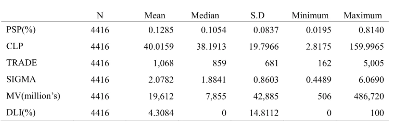
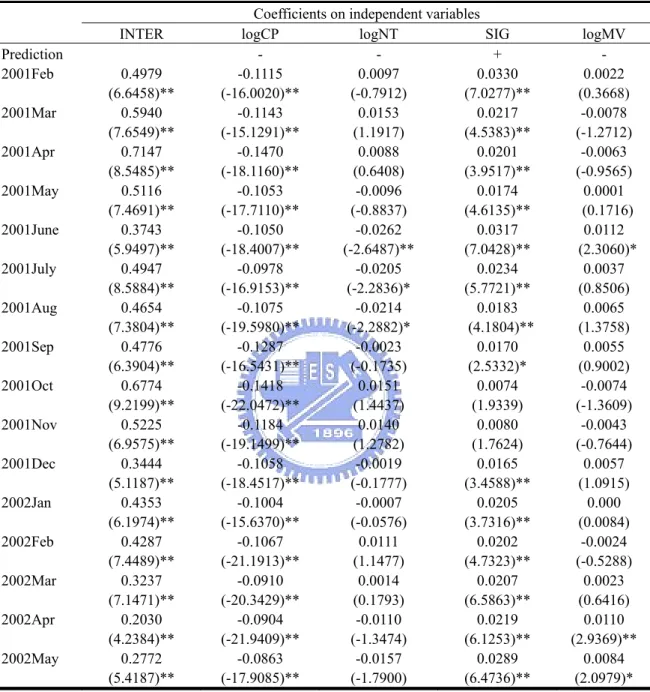
(29) 4. Empirical tests and results. 4.1 Sample characteristics. Our sample period extends over the 351 trading days from February 2001 to June 2002. The sample is divided into two subperiods: the first period is from February 2001 to September 2001, and the other is from October 2001 to May 2002. In this paper the period 2, October 2001 to May 2002, be elected the period of high financial distress costs. Table 1 presents descriptive statistics, such as the mean, median, standard deviation, minimum and maximum of selected variable for pooled data. Pearson correlations coefficients of selected variable for pooled data are given in Table 2. For CP, NT, and MV, there is negative correlation to percentage bid-ask spread. In the other hand, SIG and DLI have positive relation to percentage bid-ask spread.. 4.2 Results of cross-sectional regression. Firstly, we inspect that if the percentage bid-ask spread of the sample firms is related to the determinants of spreads, such as CP, NT, SIG and MV, found in Stoll (1978), Welker (1995), Stoll (2000), and Agrawal, et al., (2004). The monthly regression results using ordinary least squares estimation is shown in Table 3. For most months, the coefficients of close price (logCP) and volatility (SIG) are significant at the 0.05 level of significance and the signs of the parameters of the two explanatory variables are both consistent with that we mentioned above. There is negative correlation between logCP and percentage bid-ask spread; otherwise SIG has positive relation to percentage bid-ask spread. Conversely, the coefficients of the 22.

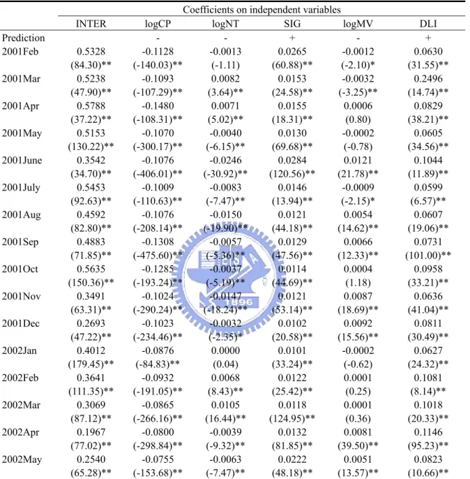
(30) number of trading (logNT) and stock’s market value (logMV) are insignificant for most months. Moreover the primary variable of interest, DLI, is put in regression equation Eq. (10). Table 4 presents the monthly regression result of PSP against four control variables and one key variable of interest using generalized least squares estimation under heteroskedastic. Roughly speaking, the coefficients of all explanatory variables are obviously significant with p-value of 0.000 at the 0.05 level for each month. The exceptions are the estimators of logNT and logMV 13 . Like our prediction, the coefficients of logCP, logNT and logMV are negative and in contrast the coefficients of SIG and DLI are positive. DLI reveals a strongly significant positive relation with PSP in each month, indicating that terrible financial condition increases the percentage bid-ask spread.. 4.3 Results of panel data regression. Because the omitted variable may be presence in Eq.(10), ordinary least squares estimation is not expected to consistently estimate any coefficient on independent variables. Unobserved effects panel data model is one of ways to address the problem. We make an effort to reduce the unobserved effects by panel data regression using fixed effects estimation. Panel data sample is also split up into two periods to demonstrate whether the results are any more significant in the period with high financial distress costs. In Table 5 is the result of panel data regression. The sign of MV’s parameter is positive unlike the expected direction. The parameter of logPDLI is totally. 13. The coefficient of logNT is insignificant in February 2001, January 2002 and June 2002. The coefficient of logMV is insignificant in April 2001, May 2001, October 2001and January 2002. 23.

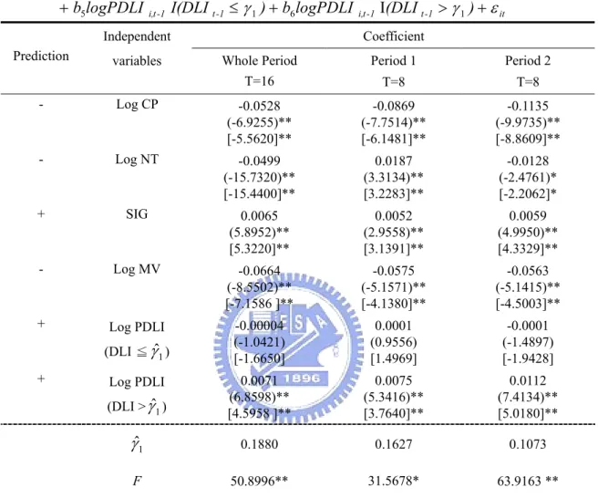
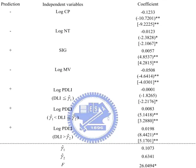
(31) insignificant. The insignificant results of the effect of DLI and unexpected sign of MV’s parameter in Table 5 might be due to the non-linear relationship between these two variables. Particularly, the model in Table 5 might be mis-specified if a significant threshold effect in DLI exists.. 4.4 Results of panel data threshold regression. For avoiding the singular matrix, in Eq.(14) as well as Eq.(15), the regressor logPDLI is introduced to replace DLI in Eq.(10). Table 6 comes out some result for ∧. panel threshold regression for each period, including estimators of threshold γ 1 and ∧. γ 2 , and the test statistics F. The estimator of threshold is 0.1880 in whole sample period, 0.1627 in period 1 and 0.1073 in period 2. Except for logPDLI of first regime, the coefficients on the other independent variables are extremely significant at 5% or even 1% level. The sign of each parameter is almost coincidence between the estimator and prediction. Three points are noteworthy in the result of Table 6. The primary estimates claim that there is positive relation between logPDLI and PSP, and “high default risk” regime possesses the enormously significant and higher coefficients than “low default risk” one no matter any period. This indicates that firms in high default risk regime heavy increate more liquidity cost than those in low default risk regime. Secondly, the coefficient of logPDLI for high default risk regime is about 1.5 times bigger in period 2 than in period 1. We demonstrate it is indeed that default risk obviously increases more liquidity cost for the period of expected high financial distress costs. In addition, the sign of MV’s parameter turns positive unlike the unexpected direction in Table 5. For period 2 we find robust evidence of a double threshold effect in Table 7. 24.

(32) There is overwhelming evidence that there are two thresholds in the regression ∧. ∧. relationship in period 2, γ 1 =0.1073 and γ 2 =0.6341. Compare the coefficient of three regimes14, the “very high default risk” class gets the highest coefficients, 0.0198, about twice higher than “high default risk” class and 200 times higher than “low default risk” class. However, Table 5 reports the coefficient of logPDLI without using threshold fails to significant. If we didn’t contemplate threshold effect, the effect of default risk on liquidity would be seriously mis-specified or undervalued. Looking at Table 6 and Table 7, the conventional OLS standard errors and the White-corrected standard errors are almost close, meaning that there is certainty in the estimate. Although in Table 7 the conventional OLS standard errors and the White-corrected standard errors on last two coefficient are considerably different, with the White-corrected ones roughly 1.5 times as big, the t-value with White-corrected standard errors is still large enough to be significant.. 14. The table of percentage of firms which fall into the three regimes each month for double threshold model is shown in the appendix, Table A.3. 25.

(33) 5. Conclusion. Our empirical result, firstly, points out DLI reveals an extremely significant positive relation to percentage bid-ask spread for each month in Table 4, proving DLI is one of the primary determinants of liquidity cost. This is to say, when financial condition is exacerbating, the percentage bid-ask spread increases, indicating financially troubled firms suffer the cost of reduced liquidity. The kind of relation between financial performance and equity liquid situation is consistence with the argument of Agrawal, et al., (2004) which demonstrates the higher spreads for firms experiencing financial dilemma are the result of an increase in informed trading in the stocks of these firms. It is more interesting that especially during the period of expected high financial distress costs, the increasing credit risk of poorly financial condition firms will contribute to the percentage bid-ask spread to raise more than usual period (see Table 6). Even though DLI is not huge distinction between period 1 and period 2, it does make higher liquidity cost in period 2. On an interesting basis we consider it is indeed in the period of Enron crisis that default risk obviously increases more liquidity cost. In addition, the credit risk of firms falling into very high default risk regime strongly increate more liquidity costs than those in low default risk regime, and this phenomenon is very obvious as the presence of high financial distress costs is severe. From what we have mentioned above, the result of this paper asserts some important meaning for investors. In the beginning, as the presence of high financial distress costs is expected, default risk obviously increases the cost of liquidity more than time of lower financial distress costs. Because the relation between default risk and equity liquidity becomes stronger as the financial distress costs are higher, the happenings of firm’s bankrupt and enormous dump of prices are generally clustered, 26.

(34) especially firms with deteriorating financial condition. This is the reason why the worse equity liquidity is able to precipitate default of poor performance firms and corporate scandal and listed company bankruptcy events always appear in a clustered chain reaction. Moreover, dissimilar degrees of credit risk are able to manipulate the liquidity cost in enormously diverse weights. Security liquidity measures the cost of taking ownership positions in firm’s equity. A stock with lower liquidity cost is always close to having excellent marketability that benefits investors greatly by allocating their ownership positions in lower cost. By and large, higher spread usually accompanies higher trading cost and bringing down the stock price. Vassalou and Xing (2004) assert stocks with both of higher default risk and smaller size or higher book-to-market ratio possess greater equity return. Moreover, according to our findings, it is suggested that higher default risk stocks in small size or high BM are particularly noteworthy when the mental situation of expected high financial distress generally exists in stock market. And auspiciously default risk level of all stocks could be classified into two or three classes according to the thresholds of DLI estimated in this paper. The stock price of those “very high default risk” category will go to down rapidly because of higher liquidity costs, so it will be correct and elegant strategy to sell or short those stocks lying in the “very high default risk” category.. 27.

(35) REFERENCES. Agrawal, V., Kothare, M., Rao, R. K. S., and Wadhwa, P., 2004, “Bid-ask spreads, informed investors, and firm’s financial condition,” The Quarterly Review of Economics and Finance 44, 58–76. Altman, E. I., 1968, “Financial ratios, discriminant analysis and the prediction of corporate bankruptcy,” Journal of Finance 23, 589–609. Altman, E. I. 1984, “A further empirical investigation of the bankruptcy cost question,” Journal of Finance, 39, 1067–1089. Amihud, Y., & Mendelson, H. 1980, “Dealership market: Market-making with inventory,” Journal of Financial Economics 8, 31–53. Bagehot, Walter(pseud.), 1971, “The only game in town,” Financial Analysis Journal, 27, 12-14. Benston, G., and Hagerman, R. (1974), “Determinants of bid-asked spreads in the over-the-counter market,” Journal of Financial Economics, 1, 353–364. Black, Fischer, and Myron Scholes, 1973, “The pricing of options and corporate liabilities,” Journal of Political Economy, 81, 637–659. Black, F. , 1986, “Noise,” Journal of Finance, 41, 529–544. Brook, Y., & Rao, R. K. S. 1994, “Shareholder wealth effects of directors’ liability limitation provisions,” Journal of Financial and Quantitative Analysis, 29, 481–497. Chan, K.S., 1993, “Consistency and limiting distribution of the least squares estimator of a threshold autoregressive model,” The Annals of Statistics ,21, 520-533. Copeland, T. E., and Galai, D., 1983, “Information effects of the bid-ask spread, “Journal of Finance, 38, 1457-1469. DeAngelo, H. D., & DeAngelo, L. 1990, “Dividend policy and financial distress: An 28.

(36) empirical investigation of troubled NYSE firms,” Journal of Finance, 45, 1415–1432. Demsetz, H., 1968, “The cost of transacting,” Quarterly Journal of Economics, 82, 33-53. Easley, D., Kieffer, N. M., O’Hara, M., & Paperman, J. B. 1996, “Liquidity, information, and infrequently traded stocks,” Journal of Finance, 51, 1405–1436. Gilson, S. C. 1989, “Management turnover and financial distress,” Journal of Financial Economics, 25, 241–262. Glosten, L. R., and Milgrom, P. R., 1985, “Bid, ask and transaction prices in a specialist market with heterogeneously informed traders,” Journal of Financial Economics, 14, 71-100. Hansen, Bruce E. 1999, “Threshold effects in non-dynamic panels: Estimation, testing, and inference,” Journal of Econometrics, 93, 345-368. Huang, R. D., and Stoll, H. R., 1994, “Market microstructure and stock return predictions,” Review of Financial Studies, 7, 179-213. Huang, R. D., and Stoll, H. R., 1996, “Dealer versus auction markets: A paired comparison of execution costs on NASDAQ and the NYSE,” Journal of Financial Economics, 41, 13-357. Kyle, A. S., 1985, “Continuous auctions and insider trading,” Econometrica, 53, 1315-1335. Lang, L., Stulz, R. M., and Walking, R. A., 1989, “Managerial performance, Tobin’s Q and the gains from successful tender offers,” Journal of Financial Economics, 24, 137–154. Lindenberg, E., and Ross, S., 1981, “Tobin’s Q ratio and industrial organization, ” Journal of Business, 54, 1–32. Lin, J.-C., Sanger, G.C., and Booth, G., 1995, “Trade size and components of the 29.

(37) bid-ask spread,” Review of Financial Studies 8, 1153-1183. Merton, Robert C., 1974, “On the pricing of corporate debt: The risk structure of interest rates,” Journal of Finance, 29, 449–470. Odders-White, E. R. and Ready, Mark J., 2004, “Credit Ratings and stock liquidity,” Review of Financial Studies, forthcoming. Stoll, H. R., 1978a, “The supply of dealer services in securities markets,” Journal of Finance, 33,1122-1151. Stoll, H. R., 1978b, “The pricing of security dealer services: An empirical study of NASDAQ stocks,” Journal of Finance, 33, 1153-1172. Stoll, H. R., 2000, “Friction,” Journal of Finance, 55, 1479-1514. Tinic, S., and West, R. 1972, “Competition and the pricing of dealer services in the over the counter stock market,” Journal of Financial and Quantitative Analysis, 7, 1707–1727. Titman, S. 1984, “The effect of capital structure of a firm’s liquidation decision,” Journal of Financial Economics, 13, 137–151. Vassalou, M., and Xing, Y. 2004, “Default Risk in Equity Returns,” Journal of Finance, 59, 831-868. Warner, J. B. 1977, “Bankruptcy costs: some evidence,” Journal of Finance, 32, 337–347. Weiss, L. A. 1990, “Bankruptcy resolution: direct costs and violation of priority of claims,” Journal of Financial Economics, 27, 285–314. White, H. 1980, “Aheteroskedasticity-consistent covariance matrix estimator and a direct test for heteroscedasticity,” Econometrica, 48, 817–838. Wruck, K. H. 1990, “Financial distress, reorganization, and organizational efficiency,” Journal of Financial Economics, 27, 419–444.. 30.

(38) TABLE 1. Descriptive statistics of selected variable N. Mean. Median. S.D. Minimum. Maximum. PSP(%). 4416. 0.1285. 0.1054. 0.0837. 0.0195. 0.8140. CLP. 4416. 40.0159. 38.1913. 19.7966. 2.8175. 159.9965. TRADE. 4416. 1,068. 859. 681. 162. 5,005. SIGMA. 4416. 2.0782. 1.8841. 0.8603. 0.4489. 6.0690. MV(million’s). 4416. 19,612. 7,855. 42,885. 506. 486,720. DLI(%). 4416. 4.3084. 0. 14.8112. 0. 100. PSP = the monthly average percentage bid-ask spreads for company i CLP= the monthly average close price for company i TRADE= the monthly average of the number of trade for company i SIGMA= the standard deviation of daily stock returns for a month for company i MV= market value of company i DLI= Default Likelihood Indicators of company i N= the number of observation. TABLE 2. PSP CLP TRADE. Pearson correlations coefficients of selected variable PSP. CLP. TRADE. SIGMA. MV. DLI. 1.00000. -0.5991. - 0.0665. 0.4142. -0.0991. 0.3041. (<.0001). (<.0001). (<.0001). (<.0001). (<.0001). 1.00000. 0.1838 (<.0001) 1.00000. -0.2895 (<.0001) 0.2064 (<.0001) 1.00000. 0.2110 (<.0001) 0.6439 (<.0001) -0.0601 (<.0001) 1.00000. -0.0156 (0.2793) 0.0125 (0.3836) 0.2338 (<.0001) -0.0616 (<.0001) 1.00000. SIGMA MV DLI. 31.

(39) TABLE 3. Cross-sectional regression results. The monthly regression of PSP against four control variables (logCLP, logTRADE, SIGMA, logMV) is estimated by ordinary least squares estimation.. PSPit = a + b1 log CPit + b2 logN T it + b3 SIG it + b4 log MVit + ε it INTER Prediction 2001Feb 2001Mar 2001Apr 2001May 2001June 2001July 2001Aug 2001Sep 2001Oct 2001Nov 2001Dec 2002Jan 2002Feb 2002Mar 2002Apr 2002May. 0.4979 (6.6458)** 0.5940 (7.6549)** 0.7147 (8.5485)** 0.5116 (7.4691)** 0.3743 (5.9497)** 0.4947 (8.5884)** 0.4654 (7.3804)** 0.4776 (6.3904)** 0.6774 (9.2199)** 0.5225 (6.9575)** 0.3444 (5.1187)** 0.4353 (6.1974)** 0.4287 (7.4489)** 0.3237 (7.1471)** 0.2030 (4.2384)** 0.2772 (5.4187)**. Coefficients on independent variables logCP logNT SIG + -0.1115 0.0097 0.0330 (-16.0020)** (-0.7912) (7.0277)** -0.1143 0.0153 0.0217 (-15.1291)** (1.1917) (4.5383)** -0.1470 0.0088 0.0201 (-18.1160)** (0.6408) (3.9517)** -0.1053 -0.0096 0.0174 (-17.7110)** (-0.8837) (4.6135)** -0.1050 -0.0262 0.0317 (-18.4007)** (-2.6487)** (7.0428)** -0.0978 -0.0205 0.0234 (-16.9153)** (-2.2836)* (5.7721)** -0.1075 -0.0214 0.0183 (-19.5980)** (-2.2882)* (4.1804)** -0.1287 -0.0023 0.0170 (-16.5431)** (-0.1735) (2.5332)* -0.1418 0.0151 0.0074 (-22.0472)** (1.4437) (1.9339) -0.1184 0.0140 0.0080 (-19.1499)** (1.2782) (1.7624) -0.1058 -0.0019 0.0165 (-18.4517)** (-0.1777) (3.4588)** -0.1004 -0.0007 0.0205 (-15.6370)** (-0.0576) (3.7316)** -0.1067 0.0111 0.0202 (-21.1913)** (1.1477) (4.7323)** -0.0910 0.0014 0.0207 (-20.3429)** (0.1793) (6.5863)** -0.0904 -0.0110 0.0219 (-21.9409)** (-1.3474) (6.1253)** -0.0863 -0.0157 0.0289 (-17.9085)** (-1.7900) (6.4736)**. For each month the first row in the “coefficients on independent variables” column gives the estimated coefficient, and the second row is the t-values OLS S.E. * Level of significance is 5% ** Level of significance is 1%. 32. logMV 0.0022 (0.3668) -0.0078 (-1.2712) -0.0063 (-0.9565) 0.0001 (0.1716) 0.0112 (2.3060)* 0.0037 (0.8506) 0.0065 (1.3758) 0.0055 (0.9002) -0.0074 (-1.3609) -0.0043 (-0.7644) 0.0057 (1.0915) 0.000 (0.0084) -0.0024 (-0.5288) 0.0023 (0.6416) 0.0110 (2.9369)** 0.0084 (2.0979)*.

(40) TABLE 4. Cross-sectional regression results (key regressor: DLI). The monthly regression of PSP against four control variables (logCLP, logTRADE, SIGMA, logMV) and one key variable of interest (DLI) is estimated by generalized least squares (heteroskedastic).. PSPit = a + b1 logCPit + b2 logNTit + b3 SIGit + b4 logMVit + b5 DLIit + ε it INTER Prediction 2001Feb 2001Mar 2001Apr 2001May 2001June 2001July 2001Aug 2001Sep 2001Oct 2001Nov 2001Dec 2002Jan 2002Feb 2002Mar 2002Apr 2002May. 0.5328 (84.30)** 0.5238 (47.90)** 0.5788 (37.22)** 0.5153 (130.22)** 0.3542 (34.70)** 0.5453 (92.63)** 0.4592 (82.80)** 0.4883 (71.85)** 0.5635 (150.36)** 0.3491 (63.31)** 0.2693 (47.22)** 0.4012 (179.45)** 0.3641 (111.35)** 0.3069 (87.12)** 0.1967 (77.02)** 0.2540 (65.28)**. logCP -0.1128 (-140.03)** -0.1093 (-107.29)** -0.1480 (-108.31)** -0.1070 (-300.17)** -0.1076 (-406.01)** -0.1009 (-110.63)** -0.1076 (-208.14)** -0.1308 (-475.60)** -0.1285 (-193.24)** -0.1024 (-290.24)** -0.1023 (-234.46)** -0.0876 (-84.83)** -0.0932 (-191.05)** -0.0865 (-266.16)** -0.0800 (-298.84)** -0.0755 (-153.68)**. Coefficients on independent variables logNT SIG logMV + -0.0013 0.0265 -0.0012 (-1.11) (60.88)** (-2.10)* 0.0082 0.0153 -0.0032 (3.64)** (24.58)** (-3.25)** 0.0071 0.0155 0.0006 (5.02)** (18.31)** (0.80) -0.0040 0.0130 -0.0002 (-6.15)** (69.68)** (-0.78) -0.0246 0.0284 0.0121 (-30.92)** (120.56)** (21.78)** -0.0083 0.0146 -0.0009 (-7.47)** (13.94)** (-2.15)* -0.0150 0.0121 0.0054 (-19.90)** (44.18)** (14.62)** -0.0057 0.0129 0.0066 (-5.36)** (47.56)** (12.33)** -0.0037 0.0114 0.0004 (-5.19)** (44.69)** (1.18) -0.0147 0.0121 0.0087 (-18.24)** (53.14)** (18.69)** -0.0032 0.0102 0.0092 (-2.35)* (20.58)** (15.56)** 0.0000 0.0101 -0.0002 (0.04) (33.24)** (-0.62) 0.0068 0.0122 0.0001 (8.43)** (25.42)** (0.25) 0.0105 0.0118 0.0001 (16.44)** (124.95)** (0.36) -0.0039 0.0132 0.0081 (-9.32)** (81.85)** (39.50)** -0.0063 0.0222 0.0051 (-7.47)** (48.18)** (13.57)**. For each month the first row in the “coefficients on independent variables” column gives the estimated coefficient, and the second row is the t-values OLS S.E. * Level of significance is 5% ** Level of significance is 1%. 33. DLI + 0.0630 (31.55)** 0.2496 (14.74)** 0.0829 (38.21)** 0.0605 (34.56)** 0.1044 (11.89)** 0.0599 (6.57)** 0.0607 (19.06)** 0.0731 (101.00)** 0.0958 (33.21)** 0.0636 (41.04)** 0.0811 (30.49)** 0.0627 (24.32)** 0.1081 (8.14)** 0.1018 (20.33)** 0.1146 (95.23)** 0.0823 (10.66)**.

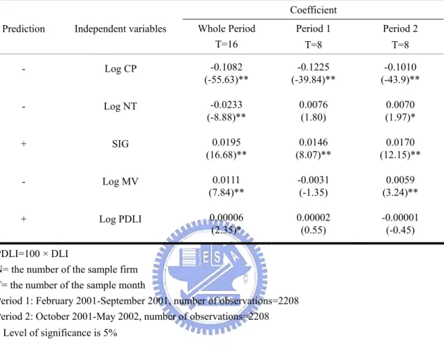
(41) TABLE 5. Results of panel data regression model (key regressor: PDLI). Panel data regression of PSP against four control variables (logCLP, logTRADE, SIGMA, logMV) and one key variable of interest (logPDLI) is estimated by fixed effect approach. N=276. PSPit = a + b1 log CPit + b2 logN Tit + b3 SIG it + b4 log MV it + b5logPDLI it + ε it Coefficient Prediction. Independent variables. Whole Period T=16. Period 1. Period 2. T=8. T=8. -. Log CP. -0.1082 (-55.63)**. -0.1225 (-39.84)**. -0.1010 (-43.9)**. -. Log NT. -0.0233 (-8.88)**. 0.0076 (1.80). 0.0070 (1.97)*. +. SIG. 0.0195 (16.68)**. 0.0146 (8.07)**. 0.0170 (12.15)**. -. Log MV. 0.0111 (7.84)**. -0.0031 (-1.35). 0.0059 (3.24)**. +. Log PDLI. 0.00006 (2.35)*. 0.00002 (0.55). -0.00001 (-0.45). PDLI=100 × DLI N= the number of the sample firm T= the number of the sample month Period 1: February 2001-September 2001, number of observations=2208 Period 2: October 2001-May 2002, number of observations=2208 * Level of significance is 5% ** Level of significance is 1% For each month the first row in the “coefficients on independent variables” column gives the estimated coefficient, and the second row is the t-values OLS S.E.. 34.

(42) TABLE 6. Results of single threshold model (key regressor: PDLI). Panel data threshold regression of PSP against four control variables (logCLP, logTRADE, SIGMA, logMV) and one key variable of interest (PDLI) is estimated by fixed effect approach. And DLI is used to be threshold variable. N=276. PSPit = b1 log CPit + b2 logN Tit + b3 SIG it + b4 log MV it + b5logPDLI. i,t -1. I(DLI t -1 ≤ γ 1 ) + b6 logPDLI. variables. I(DLI t -1 > γ 1 ) + ε it. Coefficient. Independent Prediction. i,t -1. Whole Period T=16. Period 1. Period 2. T=8. T=8. -. Log CP. -0.0528 (-6.9255)** [-5.5620]**. -0.0869 (-7.7514)** [-6.1481]**. -0.1135 (-9.9735)** [-8.8609]**. -. Log NT. -0.0499 (-15.7320)** [-15.4400]**. 0.0187 (3.3134)** [3.2283]**. -0.0128 (-2.4761)* [-2.2062]*. +. SIG. 0.0065 (5.8952)** [5.3220]**. 0.0052 (2.9558)** [3.1391]**. 0.0059 (4.9950)** [4.3329]**. -. Log MV. -0.0664 (-8.5502)** [-7.1586 ]**. -0.0575 (-5.1571)** [-4.1380]**. -0.0563 (-5.1415)** [-4.5003]**. +. Log PDLI. -0.00004 (-1.0421) [-1.6650]. 0.0001 (0.9556) [1.4969]. -0.0001 (-1.4897) [-1.9428]. (DLI > γˆ1 ). 0.0071 (6.8598)** [4.5958 ]**. 0.0075 (5.3416)** [3.7640]**. 0.0112 (7.4134)** [5.0180]**. γˆ1. 0.1880. 0.1627. 0.1073. F. 50.8996**. 31.5678*. 63.9163 **. (DLI ≦ γˆ1 ) +. Log PDLI. PDLI=100 × DLI N= the number of the sample firm T= the number of the sample month Period 1: February 2001-September 2001, number of observations=2208 Period 2: October 2001-May 2002, number of observations=2208 * Level of significance is 5% ** Level of significance is 1% For each period the first row in the “coefficients on independent variables” column gives the estimated coefficient. In the next two rows, () and [] are the t-values respectively calculated by OLS S.E and White S.E.. γˆ. is the estimator of threshold and if p-value for F is less than the desired critical value, the null hypothesis of no threshold effect is rejected.. 35.

(43) TABLE 7 PDLI). Results of double threshold model only for Period 2 (key regressor:. PSPit = b1 logCPit + b2 logNT it + b3 SIGit + b4 logMVit + b5logPDLIi,t -1 I(DLIt -1 ≤ γ 1 ) + b6logPDLIi,t -1 I( γ 1 < DLI t -1 ≤ γ 2 ) + b7logPDLIi,t -1 I(DLI t-1 > γ 2 ) + ε it Prediction. Independent variables. Coefficient. -. Log CP. -0.1233 (-10.7201)** [-9.2225]**. -. Log NT. -0.0123 (-2.3828)* [-2.1067]*. +. SIG. 0.0057 (4.8537)** [4.2815]**. -. Log MV. -0.0508 (-4.6414)** [-4.0301]**. +. Log PDLI. -0.0001 (-1.8265) [-2.2176]*. (DLI ≦ γˆ1 ) +. 0.0083 (5.1418)** [3.2880]**. Log PDLI ( γˆ1 < DLI ≦ γˆ2 ). +. Log PDLI. 0.0198 (8.4421)** [5.1701]**. (DLI > γˆ2 ). γˆ1 γˆ2. 0.1073. F. 26.0494*. 0.6341. PDLI=100 × DLI N= the number of the sample firm. T= the number of the sample month Period 2: October 2001-May 2002, number of observations=2208 * Level of significance is5% ** Level of significance is 1% For each period the first row in the “coefficients on independent variables” column gives the estimated coefficient. In the next two rows, () and [] are the t-values respectively calculated by OLS S.E and White S.E.. γˆ is the estimator of threshold and if p-value for F is less than the desired critical value, the null hypothesis of no threshold effect is rejected.. 36.

(44) Appendix FIGURE A.1 PSP V.S. DLI(Mean). PSP%. DLI%. 7. 0.18. PSP%. 0.16. DLI%. 6. 0.14 5 0.12 0.1. 4. 0.08. 3. 0.06 2 0.04 1. 0.02 0. 0 200103. 200104. 200105. 200106. 200107. 200108. 200109. 200110. 200111. 200112. 200201. 200202. 200203. 200204. 200205. Month. PSP V.S. DLI(Median). PSP%. DLI%. 0.16. 0.002. PSP%. 0.14. DLI% 0.12 0.001. 0.1 0.08 0.06 0. 0.04 0.02 0. -0.001 200103. 200104. 200105. 200106. 200107. 200108. 200109. 200110. Month. 37. 200111. 200112. 200201. 200202. 200203. 200204. 200205.

(45) TABLE A.1 Descriptive statistics and t-test results of DLI Panel B of Table A.1 shows the average DLI of all firms in period 1 and period 2 are 4.7616% and 3.9428% respectively. In Panel B of Table A.1, the t-value is -1.34 and the p-value is 0.1827 without less than 0.05. The t-test result means that DLI for period 2 fails to significantly differ from that for period 1.. Panel A: Descriptive statistics of DLI DLI. N. Mean. Median. S.D.. Minimum. Maximum. Period 1. 276. 4.7616%. 0.0829%. 13.5339%. 0.0000%. 87.5001%. Period 2. 276. 3.9428%. 0.0006%. 12.4946%. 0.0000%. 87.5000%. Diff. 276. -0.8187%. -0.0006%. 10.3646%. -73.2764%. 79.3695%. Panel B: T-test result of DLI H0: the difference of DLI for company i between Period 1 and Period 2 equal zero Variable. N. t value. Pr > |t|. DLI(Diff). 276. -1.34. 0.1827. N=the number of the sample firm Period 1: February 2001-September 2001 Period 2: October 2001-May 2002 Diff: the difference of average DLI between Period 2 and Period 1 for each firm. 38.

(46) TABLE A.2 Tests for threshold effects This table is to show whether the threshold effect has observable influence on coefficient estimator. If p-value for F is less than the desired critical value, the null hypothesis of no threshold effect is rejected. And. γˆ. is the estimator of threshold. The F statistics for threshold effect test is strongly. significant with a bootstrap p-value under 0.05, telling us the threshold effect is functional. Test for February 2001-May 2002(Whole Period) Single threshold model. γˆ1. 0.1880 50.8996 0.0000 (20.5702, 23.9565, 33.1793). F P-value (10%, 5%, 1% critical values) Test for February 2001-September 2001(Period 1) Single threshold model. γˆ1. 0.1627 31.5678 0.01667 (21.56139, 25.9425, 36.1869). F P-value (10%, 5%, 1% critical values) Test for October 2001-May 2002(Period 2) Single threshold model. γˆ1. 0.1073 63.9163 0.0000 (22.2123, 25.4175, 33.4855). F P-value (10%, 5%, 1% critical values) Double threshold model#. γˆ1 γˆ2. 0.1073 0.6341 26.0494 0.02 (19.2688, 23.5110 , 27.9175). F P-value (10%, 5%, 1% critical values). # There is significant double threshold effect only in period 2 (October 2001-May 2002). 39.

(47) TABLE A.3 Percentage of firms in each regime by month: double threshold model We find that the percentage of companies in the “very high default risk” category ranges from 0.36% to 6.88% of the sample in each month. The “low default risk” firms range from 76.81% to 93.12% of the sample over the months. The average of percentage bid-ask spreads for each regime are 0.1197, 0.2087 and 0.2461 in that order. The “very high default risk” class has the highest average of percentage bid-ask spreads, 0.2461. This proves that the firms with higher credit risk will suffer higher liquidity cost. Firms class. DLI<=0.1073. 0.1073<DLI<=0.6341. DLI>0.6341. ASPS=0.1197. ASPS=0.2087. ASPS=0.2461. Month. No.. ％. No.. ％. No.. ％. 2001Feb. 212. 76.81%. 45. 16.30%. 19. 6.88%. 2001Mar. 257. 93.12%. 18. 6.52%. 1. 0.36%. 2001Apr. 246. 89.13%. 24. 8.70%. 6. 2.17%. 2001May. 252. 91.30%. 16. 5.80%. 8. 2.90%. 2001June. 256. 92.75%. 13. 4.71%. 7. 2.54%. 2001July. 255. 92.39%. 14. 5.07%. 7. 2.54%. 2001Aug. 253. 91.67%. 17. 6.16%. 6. 2.17%. 2001Sep. 250. 90.58%. 19. 6.88%. 7. 2.54%. 2001Oct. 238. 86.23%. 31. 11.23%. 7. 2.54%. 2001Nov. 243. 88.04%. 27. 9.78%. 6. 2.17%. 2001Dec. 250. 90.58%. 20. 7.25%. 6. 2.17%. 2002Jan. 250. 90.58%. 21. 7.61%. 5. 1.81%. 2002Feb. 250. 90.58%. 21. 7.61%. 5. 1.81%. 2002Mar. 253. 91.67%. 18. 6.52%. 5. 1.81%. 2002Apr. 261. 94.57%. 13. 4.71%. 2. 0.72%. 2002May. 257. 93.12%. 16. 5.80%. 3. 1.09%. APSP= the average percentage bid-ask spreads for each regime No.= the number of firm. 40.

(48)