Fourier and wavelet analyses of TOPEX/Poseidon-derived sea level anomaly over the South China Sea: A contribution to the South China Sea Monsoon Experiment

JOURNAL OF GEOPHYSICAL RESEARCH, VOL. 105, NO. C12, PAGES 28,785-28,804, DECEMBER 15, 2000

Fourier and wavelet analyses of TOPEX/Poseidon-derived

sea

level anomaly

over the South China Sea: A contribution

to the South China Sea Monsoon Experiment

Cheinway

Hwang and Sung-An

Chen

Department

of Civil Engineering,

National

Chiao

Tung

University,

Hsinchu,

Taiwan

Abstract.

We processed

5.6 years

of TOPEX/Poseidon

altimeter

data

and

obtained

time

series

of

sea

level anomaly

(SLA) over

the South

China

Sea

(SCS).

Fourier

analysis

shows

that sea

level

variability

of the SCS contains

major

components

with periods

larger

than 180 days

and is

dominated

by the annual

and semiannual

components.

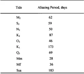
Tidal aliasing

creates

30-180 day

components

that can

be misinterpreted

as wind-induced

variabilities.

Continuous

and

multiresolution

wavelet

analyses

show

that the SLA of the SCS has

monthly

to interannual

components

of time-varying

amplitudes,

and

the

regional

slope

of SLA

is 8.9

mm

yr

'1,

which

may

be caused

by the decadal

climate

change.

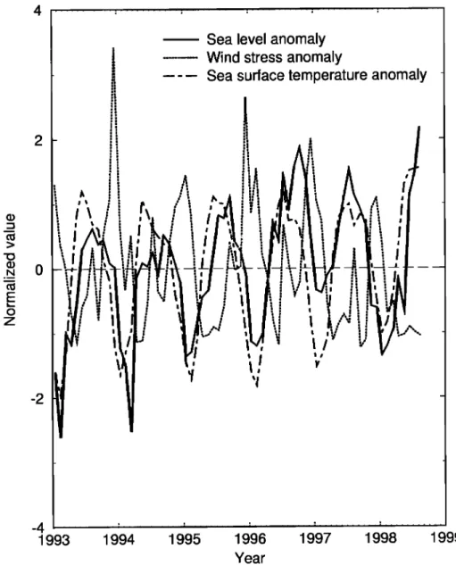
Coherences

of SLA with wind stress

anomalies

(WSA)

and sea

surface

temperature

anomalies

(STA) are significant

at the annual

and semi-annual

components.

At periods

of 2-5 years

the wavelet

coefficients

of SLA, WSA, and STA have

the

same

pattern,

but WSA leads

SLA, and STA follows

SLA. The zero

crossing

of SLA in spring

is

highly

correlated

with the onset

of the summer

monsoon.

The interannual

variability

of SLA is

curvature

from negative

to positive,

an E1 Nifio is likely

to develop.

This is a contribution

to the

South China Sea Monsoon Experiment (SCSMEX).

1. Introduction

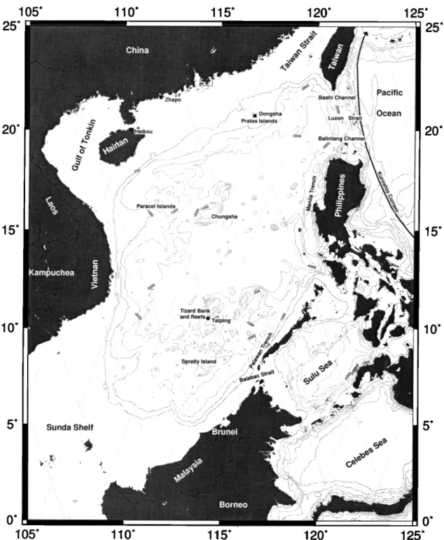
The South China Sea (SCS) is the largest marginal sea in the

western Pacific with a total area of 2,590,000 km 2. Figure 1 shows

the countries, waters, major islands and bottom features, and major

depth contours around the SCS. The South China Sea Monsoon Experiment (SCSMEX) is an international project to study the

monsoons over the SCS. The participating countries include most

countries in east Asia and southeast Asia, Australia, and the United

States. Its purpose is to "better understand the key physical processes in the onset, maintenance, and variability of the

the summer and winter monsoons over the SCS and to E1 Nifio-Southem Oscillation (ENSO) will also be studied.

2. Sea Level Anomaly From TOPEX/Poseidon

measure the height of the sea level with a repeat period of 9.9156

days. We used the T/P Version

C Geophysical

Data Records

(GDRs) from Archiving,

Validation,

Interpretation

of Satellite

Oceanographic Data (AVISO) [1996] to generate corrected sea surface heights (SSHs) from cycle 10 (December 26, 1992) to

monsoon

over

southeast

Asia

and

southern

China"

[Lau,

1997,

p. cycle

219 (August

29, 1998).

The

first

nine

cycles

were

not

used

599].

We have

joined

SCSMEX

to investigate

the

characteristics

of because

of a pointing

problem

[Fu et al., 1994].

The

orbit

we used

sea level variability over the SCS derived from the in the T/P GDRs is based on the Joint Gravity Model 3 (JGM3)

TOPEX/Poseidon

(T/P) altimeter.

We will perform

Fourier

and gravity

field [Tapley

et al., 1996]

and

has

an accuracy

of about

4

wavelet

analyses

of the T/P-derived

sea level time series. cm. The dry tropospheric

and

inverse

barometric

corrections

were

Compared

to Fourier

analysis,

wavelet

analysis

is a recently based on the European

Centre for Medium Range Weather

developed

tool that

is best

suited

for analyzing

phenomena

with Forecasts

(ECMWF)model.

The

wet

tropospheric

corrections

were

time-varying

frequencies

and amplitudes.

An extensive

body

of directly

taken

from

the TOPEX

Microwave

Radiometer

(TMR)

literature

associated

with

wavelet

analysis

has

been

developed

over measurements.

For the ionospheric

correction,

TOPEX uses

its

the past decade.

The lectures

by Daubechies

[1992]

provide dual

frequency

measurements

and

Poseidon

is based

on the

model

readers

with

both

an introductory

and

an in-depth

understanding

of of Doppler

orbitography

and radiopositioning

integrated

by

wavelets.

A practical

guide

to wavelet

analysis

is given

by in satellite

(DORIS). The CSR3.0

ocean

tide model

[Eanes

and

Totfence

and Compo

[1998].

A collection

of applications

of Bettadpur,

1995]

was used

to detide

the data.

In particular,

an

wavelets in geophysics and oceanography is given by in oscillator drift correction has been applied to the TOPEX range Foufoula-Georgiou and Kumar [1994]. Moreover, we will measurements [AVISO, 1996]. To produce SLAs for the

compute

the frequency

response

functions

and

coherence

functions

subsequent

analyses,

we first formed

stacked

along-track

SSHs

by

[Bendat

and Piersol,

1993] between

sea level, wind, and sea averaging

the point SSHs from the 210 T/P cycles.

When

surface

temperature

over

the SCS

to see

the degrees

of interaction

averaging,

the gradient

of a geoid computed

from the Earth

among these signals. The relationships of sea level variability to Gravitational Model 1996 (EGM96) to harmonic degree 360 [Lemoine et al., 1998] was used to reduce point SSHs to the nominal ground tracks selected to correspond with the tracks of

Copyright

2000

by

the

American

Geophysical

Union.

cycle

92 for

this

study.

A point

SLA

was

computed

as

Paper number 2000JC900109.

0148-0227/00/2000JC900109509.00 zlh = h- h , (1)

28,786 HWANG AND CHEN: FOURIER AND WAVELET ANALYSES OF SOUTH CHINA SEA 105 ø 25 ø ß 20' 110 ø 115 ø 120 ø 125 ø ß 25 ø 20'

15 ø -

15'

::'Kam•Uchea.

•.

" / • 'x•

•./'•

Tizard

Bank

5 ø

Sunda

Shelf

.,

./•/ :o

5 ø

',

...

: I

•' /

...

-, :,h•-' ,,-'•. •'

'

0 ø .

."'/

...

/•, , •zp•-•,•-•••:• ß

105 ø

11 O'

1150

120 ø

125 ø

Figure 1. The South China Sea and its surrounding countries and waters. Also given are selected depth contours (solid lines), the ground tracks of TOPEX/Poseidon (dots), major bottom features, and islands. Squares indicate tide gauge stations.

where h and h are point and averaged SSH, respectively. An

area-averaged SLA over a given area is the simple mean of all

point SLAs in the area, and the associated time is the central time

of the T/P cycle. In computing the simple mean we rejected outlier

SLAs using Pope's [ 1976] • - test. An outlier point SLA satisfies

=

.

(2)

where v i and • are the residual of a SLA (observation minus

area mean) and the residual's a posterior standard error,

respectively, a is the confidence level, which is 95% in this

paper,

n is the number

of point

SLAs,

and *a;•,,-2 is the critical

, value with degrees of freedom of 1 and n -2. Outlier rejection

was performed iteratively until no outlier was found, and the final

area-averaged SLA was computed from the "clean" set of point SLAs. On the basis of Figure 1, SCS depths range from less than 200 m over the continental shelf to 6000 m at the center of the

basin

and

at the Manila

Trench.

From

numerical

models

[Shaw

and

Chao, 1994] and dritter data [Hu, 1998] the SCS has two distinct

HWANG

AND CHEN:

FOURIER

AND WAVELET

ANALYSES

OF SOUTH

CHINA

SEA

... SLA4 (continental shelf of SCS)

I i i I J i i , i i i i i i , , I

1994

1995

1996

1997

1998

1999

Year

Figure

2. Time

series

of SLA

in four

areas

of the

SCS.

28,787

altimeter-observed

SSHs

over

shallow

water

will

have

larger

errors

Table

1 shows

the

statistics

in generating

the

four

SLA

time

series.

than

those

over

the

deep

ocean.

To

see

the

spatial

characteristics

of The

large

percentage

of rejected

SLAs

in SLA4

is due

to the

large

the

SCS

sea

level,

we

computed

SLA

time

series

in four

subareas

ocean

tide

model

error,

distortions

of altimeter

footprints,

and

of the SCS:

The first one

(SLA1)

is over

the deep

ocean

(depths

>

200 m) between

14.5

ø and 22øN,

the

second

(SLA2)

is over

the

deep

ocean

between

5 ø and 14.5øN,

the

third

(SLA3)

is over

the deep

ocean

between

5 ø and 22øN

(this

area

combines

the

continental

shelf

(defined

as the area

with depths

<200

m) and

between

14.5

ø and 22øN. Figure

2 shows

the four SLA time

series.

Note

that

the time

series

in Figure

2 and

other

figures

in this

paper

have

the beginning

of each

year

(January

1) labeled.

In

general,

SLA1,

SLA2,

and

SLA3,

which

are

over

the

deep

ocean,

agree

very

well

with

each

other

but

are

significantly

different

from

SLA4.

SLA3

behaves

basically

as the average

of SLA1

and

SLA2.

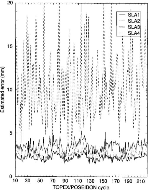
wind-driven events. Figure 3 shows the standard errors of the area

means in the four SLA time series. The standard error of an area

mean, tyro, is computed by

O'm

=

I(

• V,

2

)/n(n

--

1)

,

(3)

where v t and n are defined

in (2). By this definition

a SLA

standard error will be affected by the variability of the sea surface under study. It appears that the SLA4 error is not random and has

periodic

components

arising

from ocean

tide model

errors.

A

Table 1. Statistics of Area-Averaged SLA over the SCS

Number of selected points

Percentage of rejected points, % Mean standard error, mm

North 727 0.76 3.49 South 997 1.66 2.75

All Continental Shelf

1726 132

1.15 3.73

28,788 HWANG AND CHEN: FOURIER AND WAVELET ANALYSES OF SOUTH CHINA SEA 2O

"

• ,,

SLA1

I I,

i

, I

', ', ...

SLA2 1

',, "

" t

, t t

', ,, -- SLA4 ,,1

15

•" "

'•

" " "'•"

"

" "I ,'•,d

I Ill •l

• Ill

I II I I iI

i'• I I

tl Illll Ill

I

illl

•, II

I l

IlI

i.• rl I I I,illl . I '

I I

II •II II Illl

'Ill

?l I

I I Illl • !'I I • Ill I Ill I! I I' ii '

I, , Ill

' I Ill I I I

"•

III I II

I I III1•!

i I iii

Ii1

III !

II 1

I I I1•11

I1 1

Illl I IIIII

•

I I I 1 I

II I II

I I I •11111

Illl

I I' I , I II

I II I. i ifl

I •

I' iii'

I I II IIII

• ii Iiii,

' ii i i I Iit

II

I II I

•Ii ' ' ' • ,"1 ,, ,' '1'1' •' ', ' ,•',', •, ,,,1', ,I,,,d

II I1 '.i' I

I I Ill

III I I I ' i I

Ii:'11Ii'

I I •t II I Ij Ii

1

• 10 ,, '. ',:I',

.

,• ,•,....,'.'

..,,

,';,,I,

,

'" •.. ,,, ..

ß

•

,i ,, !"

i

", ,',

•,l,•',

!',,'

,•

,i, ,

,

,,:I1 ",,

',, ,I,,," ,l',,'

',i!' '•

I t' ,

:,,I, /

.• r..,,.

, , I .,..,, ,,',

.i ,•' •, . t•, t ,,,,,

Ii, l/ •.• I I ,I •, ,. Ui II I llll • I, II • II I1,1 I•.

,,.' ',',,,

.',, I,i ! I..,.!ii..., ,,,

.'l ', .,,,ll .

,,,. !•

,.,, • I. "'•" •'

"I I 'i'l.

I

' I

II • I

I

II

""::,',ii'

"'" ..., ""?'

',",..

"'

',

'

',¾"::' '"'"'

10

30

50

70

90

110 130 150 170 190 210

TOPEX/POSEIDON

cycle

Figure 3. Estimated errors (1 standard deviation) of the area-averaged SLA in four areas of the SCS.

spectral

analysis

shows

that

the spectrum

of the SLA4

error

is SLA1

is much

larger

than

that

of SLA2

because

of the higher

almost

"flat,"

except

at two distinct,

large

components:

the largest latitude

of the northern

SCS, which is more sensitive

to the

component

has

a period

of 59 days

and

an amplitude

of 1.2 mm, seasonal

variation

in solar

insulation

than

the

southern

SCS.

Figure

and

the

next

one

has

a period

of 27 days

and

an amplitude

of 0.8 5 shows

the filtered

SLA

time

series

that

were

computed

using

a

mm.

These

two components

have

to do with

the T/P tidal

aliasing

Gaussian

filter

with

a wavelength

of 1 year;

see

Wessel

and

Smith

discussed

below.

In addition,

the SLA2

error

is smaller

than

the [1995]

for the

definition

of the

Gaussian

filter

and

its

wavelength.

SLA1

error

because

SLA2

uses

more

data

points

than

SLA1,

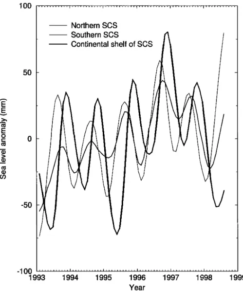
and Clearly,

the annual

components

over

the northern,

southern,

and

the

northern

SCS

has

a much

larger

sea

surface

variability

than

the continental

shelf

parts

of the

SCS

have

summer

peaks

at different

southern

SCS

[Hwang

and

Chen,

2000].

times

of the

year.

Comparing

the

phases

of the

annual

components,

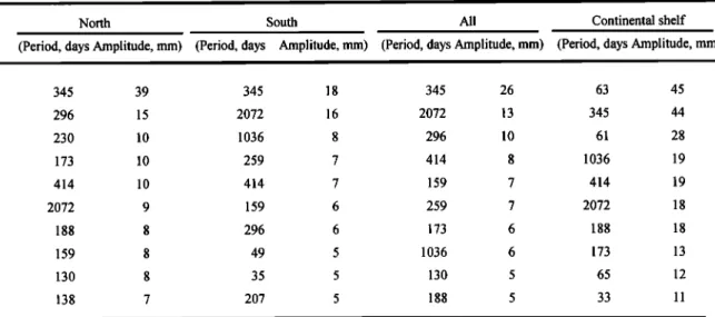
3. Fourier Spectra

of Sea Level Anomaly

3.1. Periodograms

To see the overall characteristics of the sea level variability over the SCS in the frequency domain, we performed Fourier transforms to obtain periodograms of SLA1, SLA2, SLA3, and SLA4 (Figure 4). Table 2 shows the amplitudes and periods of the

first 10 largest components of the four SLA series. All four SLA

we find that summer peaks for SLA1 lead those of SLA2 by 21

days and SLA4 by 76 days. In the four SLA time series, there are

two strong interannual components with periods of 1036 and 2072

days, which will be investigated in connection to ENSO. Again, in

all aspects, SLA3 behaves essentially as the average of SLA1 and

SLA2.

3,2. _{Tidal Aliasing in TOPEX/Poseidon}

SLA4, being over the continental shelf, has a distinct Fourier

series

have

strong

components

with

a period

of 345

days,

which spectrum

compared

to those

of SLA1-SLA3.

SLA4

has

strong

HWANG AND CHEN: FOURIER AND WAVELET ANALYSES OF SOUTH CHINA SEA 28,789 50 40 .-. 30 E E E

<t: 20

10 ':i

.

?.,

::

0 1 2 3 4 5 6 7 8 9 10 11 12 13 14 15 16 17 18 19 20

Frequency

(cycle/year)

Figure

4. Periodograms

of SLA

time

series

in four

areas

of the SCS.

Table 2. Periods and Amplitudes of the 10 Leading Components of the Four SLA Time Series Over the SCS

North South All Continental shelf

(Period, days Amplitude, mm) (Period, days Amplitude, mm) (Period, days Amplitude, mm) (Period, days Amplitude, mm)

345 39 345 18 345 26 63 45 296 15 2072 16 2072 13 345 44 230 10 1036 8 296 10 61 28 173 10 259 7 414 8 1036 19 414 10 414 7 159 7 414 19 2072 9 159 6 259 7 2072 18 188 8 296 6 173 6 188 18 159 8 49 5 1036 6 173 13 130 8 35 5 130 5 65 12 oo • 1 1 138 7 •" 5 Ioo 5

28,790 HWANG AND CHEN' FOURIER AND WAVELET ANALYSES OF SOUTH CHINA SEA

1993 1994 1995 1996 1997 1998

60 _{.... • --] ,- 14½ I- $-• +-•..1. • ... 4- • 4.- •.-i- i ' ' ',-4 .•- •--: ... l--L.-•-.•..,•'•k • ... ,.;•Z•' "•LL-.L..I-I-•.:.•...L .;-.. [.¾', ' ' ' .'}

- F -• • ' / ' • • t ' ß , i • ß ' • ß : • • - • ' ' i -•-• • •-•- ;- • •' • ß I : t ' :• t • i • ' ' • • , • ß

,-' ... [ '. .... i ... ;.-4 .: ... i--i ... -]• -.•. 4--r.- --. •--• q -, •--,-,--- .-,.-•.i ... i...• ... •d.-i --I ...

a tt*. ,,:,,:- ,,, , .... ... ß r,,::,- ,, .... l

54 ( ) ....

...

... ...

...

, ...

, ...

...

, ...

...

48 1-4 -•--P .[-•4-14--i-PJ-L4•-• z. ! ::-!-.-i--:r--•.- :•--[. 4- !..-•-. i--•q.•-P.i-P..L_•-'• -•%•. -••.4•-.P.k.L..L.-p+ ' ..;....i....:....i..4...!...

•[, •-4- •--*--• &.•._.•.• ._•..- ...,;;_& .[_•_ • ... • ... &..[..•..,•.,•,-[ ... ; •....• ... : . • .... [.-•.•,...•_• ... • ... • ... &..L_•

- -• " • •- • "•'• ß -•'-'•* •--'*• " s •.' '? ' • -- ' ,. -- .r .... . '•.'•' •'*•'-:-• -"r- ;-'• ... • ... • .... • • ....

O 24 / • • F • _{•'*-•"• I'=½ •-• •'-'F•} •'• , •'"r-•-•-•'-F"ir'-•- _{.... • '--i-' *"T"•-•"r ' r •-•-•} •-• •W'F'• ... _{... •- •---•' -•--:--•-+---•-.r-•--} %'•r"F-'c' r-'i • •'"Fz"'F _{'r i- =-} -r-F • "T"i". • •- • 'i' •-'7" _{i -i--• + -- i•-f.-•--, ... i.--f- .• -i--} wr.-,--

ß i i ! ß . : • . • : : ! ! : • • • i 1 : : i ß : i - • - i • • . i : : . : . ! ! • i i I

" • ... [' 'F'I .-q--r.---,--.• ... '"'+-"-•-T '+ ... * ... •-"-,'--½ -1-•-• .... i ... •----r--q--.f .-.I -• -i ... i ... i ... i ... i' '-•"! ... '""*""i ....

•,, z_i j_, X_•.J._L LL Li.. • i..%.i._L • ..'__Li., '•._L i' i._L LJ '[ J ... •...: ==...•._i j. i_i_L' _L.L..t%.L_' _[.•_.t ..• •..

3 • _{ß '} ,-- _:• i = r -'• _{-[ ' •.-. ' ß •-•--} r-•"i ,'- i-"=T'•?'-w'•F ', •", T-mr _{-,-{-L • i .... L..-.:•-I-..½ ... •-,} • -'r-F'r" _4•.4.•- • r c' r"t r .... 7r' %-r' _{!--•-•.-=-+-O-.!.- =-.-•4. -::- !.-.H-..• .... '. -•-4--+-: --.-} t-? 'rw-rm-r'? r ... rw T •-r'

6O 54 48 42 36 3O 24 18 12 60 ß : : . , ß : * : ß : : : : ß - : : : • : ..: • • r t':- , • i ß • , - : i : : : : ß : : : : i : • .. ß t • • : 60 . _ •.---i --t.-~4.--i----,- -i - i---•-~ t---I--..i-. i--- ,-- -i -4. -i--.- i- , ---i-- -, --; --{-.-{.--,--.-4.-.-•.. ,---,---•4---,•-...I.•-.,.,-,.-..I.,,,4,r -. ,.•,.-,--..I-...,,..-..i....i,.- ..i. -i---.i-.-i-- ..i-.-i---.4.--i----.•--.-,,---•,..-4.--} .-.•-..-•--[--.:-i ,.4. (•. I --,-,--,- ,--•..---+-!-?-,-,-'t ... ,-'--,'-' .--',' ': -, ... ,-',--?'-,'---," -,-""+-•-'", "' .-'=','"".'-' ,-:"'i' -,--,--,---,--4-.,----.,---,----:----,--: ... !--..-!-,--, .--t ',' 54

54 v ' ! I i ! ": : i i i "' : I "i : ! • * : ' ': } I-•-: : ' t*"i I ! • ' • i%"I - : : : •.-,- : : : : • .*-,-! : z t ß : : : : : : I : • • : . : ;.- ß . . 3 ' i ! i ! ! ! i t : * i '• i ! *• ß i I : : : . : ; ! ! . : : ß ß

• /' •- *•'-"--q-'"•'---• "--'--•-'-" ... -" ... •-'" ... •' +---'- -'--*'"1'--'--- '- L.•-• ... ,--,-- r ... , ... +-~•---, ... •-F•i•.

,__, _. : ' LL LI.2... L..•LL •-_LU •.J-%J-L..L-L-L ',. .-L •....L L_L .[ _.L .L..i..j.i_ L4._.L_LL_Li...[". i-...L..L.J _L ..L.. t_.L .L_:..4 ..•._i...L2-.-"-L.L.2.. •.L. .... 48

48 ...,,: _{. -,---•-.•-i- F ' -•-q.-.•.-.•-'!--.•-4-•-i--.•-F•.--i--•:-.•--.•} ,.:: ,:,:::,:,,:..,,,,::,:,:,,,, _{' !--'--•---F---.•-!---i---.:-•--.•-!---!--.•-•} , _-'-.-.P--'.- , ,,,,.:,.:,-.,,,,:. _{4. _•'-+.•_q_.F-,....•..•_•-:_..•} , _ß

42 _:•.L _{• .i__•_•__i._.;_4.• _• ß _•.•.•_•4•-,__t•.•} ... ,•:_.•_;•.,.•:_: • ß • ... ... • '••.'-.:•.4•4-k•. s • • • • _.... -i ,•_ !--•-•-..L. P-i- _{i._•L_-;•....i....•} ß t ß ß . • - . _{.... i._.•_ i....•} ! -k .... 4. --'.•-•-i-'.•-.L-i-:•k _{... •. •-•- • .l..-.•.•,-.•-•.[,..• .... •-.i..-•i} • • , r ß ß ß t ß •-..:--P.½4--.L•--i--i--:.•--P ß , • ß ß • • ß ß • • _{•_4._•_, ...} '• •.4 --•: _{..4 i} ß , --• • _{,_} • 42

36 ... :- ... ',---'• ... • ... ' ... .•'-'• ... ' ... : ... • ... '*• .... r ... ,--.' ... :-.'- ... 36

ß ß : : - : :.. : ; * : : i : : • : : • : . . : m. : , : : i : : • : .• : • : : : : r ß T 't: t•l !---? .--:'--? ":"":--T-r--. : . •

• , : - - ß -. - _ .... :_ .• .... •...•_._ ... ... , :•...:. • :_.-_. ß ... .._ ._....:...;•.•u ..: .... : .- ...:. --...-.._.: .•-....:..._,.• ... L ...- ...

-,-, 30 '.---• _{• _,._:-..3._} ... _{.... •_i...LJ_2_} •-+.-•-•-+-. _!--L--:..-: -i .... •--':- !--,4-: _{.•L. L_L.-_.i...L_L..L....•} ... i .-•.--; ... _{.Z...:..._2._:-...!...:;..•.._L.J...L.} ';--k..:--:--:---;---+-i--. :--e--'•-4----:.--:.--."----•+-i-. _{:,._LJ_.L...'.'._L...LL.L_':} 4- ... _{..i_.[.4_LJ_.•....LL_•_;...i....L.i...•....L_L} '--...[.~•--: ... .t.-:.4-.:-...I...•4.-:•..4-.•-,..-+ _{4_ •} 30

f t =-T- -- '[- -- u -• ----'-:- ß •.--.-r .--r--: ... :---•---: -•- :--'-r ... •._ ,- ,•..._:..._= ._..:.. ... .•-•...a. ... .•.

O 24 •..L• _!.. ... L• • -', L•_•-._L___i_L_L_L;_•_ !. ... L..-_::_.:._,i....L_:' .:..J-"•-`-.•--•:•...:-&..L...L-.:--..L-.`-...•`-L•.-.•.:-.L.L.-...-.L.:..--L-L.! ;...,•...,.'_,'..._i_.i_..i....•_._•_• , . 24

: . ; . :

l:::: 18 __Z_T-'.. ß ::_:..'-:_Z_--::_E • • i •- ;7.'7.Z.•.-7•_T.F'.-_UC-' -L-•']'œE-r7.-F-•,'.]Z-E:•.-.:- ' '• .... : F-r::...•ZZ•27;Z!•'4L-.F•;.r-:..-'"E;]E:.•E'L4- 18

-o 12 ...

' ...

.: ...

ß i : ' ' ': ...

12

': ... t ... '- "t• ... • ... '•'"' ' - --"' ... :- ... T ... :' "-' -•" ...

O i -•'-: i" i :"t. -::-'•-i-i ! • • !-'•-'.r!'T-½"::.-'1-i .-,TT'.:.-". '--i F-h-i, .'--: ; i'"'t-• ?r-h!-h:. :--;"½-i'"t

ß • 9 .• +-4.-: -f .... f-": -'+---=-f-i--: ... -.:---? .+-:-?+.-..-.•-•--.:..--+..½-,:--:.-. ;-..r-: ... P•:-'-r-'•--'•-,-'-•-":--:'•- *--•.--•-•-•-t'-* ... :- ... •-?-:.-• -' ß v- 9 --*-'T'w -"r-,"'r-r-:"-..-:---r.-r----r"•-'-, '• "-:~?---.'-? , r'"•"r'-,-'T-w r-".:'"'r-.:-'"r'-:-r•.--r-.:'"'r--: ... c-r-?", ':'-:--'??'-r"'?-7. ':"T"JF-r"T • ß

(1)

t

, , • : -: -:..!

....

,. ,_• , * : L -• :' •. : : .,i_,L_L

:. _:

'-'

•. :-.J

i..

L.:_

i..

:...i

2 ...:....•_.•

•..•.

L-"...,..i_:._

i .s • i_i_:..L.~L

,' • ..:..:...•.,

! 1: f

•, i : T-• -,'?Ti':.. ;-• i'-'F '-'!-i'"•-i ,W'T. i: !'• '!-f-iT !-i 'i 'i "• •' '".-- iii f¾.'!'-:: t ['i FTf"FF !' ;"i ',-'!-;•'i"• T':• ],: F

13_ 6 ...

6

: ' : : : i ,; [ : : } ' ß : : i • ' i i i '• ; : i * : r: : : •""•:

* : : • • : ß

.•'•

-?-!"i

: : : i i = : i : --

: .

,..•.1- .•,..:f':,,,..,

,•:,,i,.•,...,..i•.,!:,:•,T•

...

øF_L,:..,•:.•..,,:,•,,:....,,

•

'q ' F.'F'r

!'.-'F'f

i'-:--7'-•

: 'T":7'qT'•

....

FT'•

• i'--:-fW'.-

f-•-'--.'.--:

F'T.T-i

C-iTTF'=

;-i-.?'i

i"'i

i"¾':.7-i'"i

':-

?'•'-[T'-f-i-FTT

3 -• .... : . : . .- • .... 'r•--• ',"-""'?-'-'-, ... "-'---'.- ß ß ; ,• : : . - - . . • . s ,- ß : ... r-:-',- ... . : . . - . : . ?--.- ... : . . . • . :--,-,--,-,-? ; : : I, : . ... . •---.--,--.-- . : : ß : : ... :---,- : . . • 3

-I'..--'"-e--":,-'-"'.•--+• ,L.'? :--'"'--i--- .-'--:--"•-' '."'."!-- .... e"-i:."-•:' "•-. -'-' .: .-'--:'W---"--- •'"= "'•;-'•-: '. '•' '• •---:--'--:' .-I•:-:.--'•-.:--':-'• .... F-"I- ..• - ß . - - - . . : : : : - : - I : : . : : - : - ß ß : I I : o ß . : : - : - . : : t : : ß . : t : : ' L I I

1993 1994 1995 1996 1997 1998

Time (year)

I

0 5 10 15 20 25 30 35 40 45 50 55 60 65 70 75 80 85 90 95 100105110115120125130

Plate 1. Wavelet coefficients of (a) SLA, (b) wind stress anomaly, and (c) sea surface temperature anomaly over the $CS. The period of a wavelet coefficient is in the sense of Fourier analysis. The unit of coefficients is arbitrary. A coefficient of 130 means that the corresponding wavelet has the maximum similarity with the signal,f(t); a coefficient of 0 means that the wavelet has the maximum similarity with -fit); a coefficient of 65 implies the least similarity

HWANG AND CHEN: FOURIER AND WAVELET ANALYSES OF SOUTH CHINA SEA 28,791 1980 1982 1984 1986 1988 1990 1992 80 ' ' ' [ ' :

(a) , i

i

'.

i :,

t

• I ! I i '

i ß ' "

!

ß

60 ...

l ...

i ... , ...

7

...

.T-

...

r

...

T'

t ...

2O

I

,i !

,..

,

•

•

,: x i

ix i

,'

.x {

30 ...

• ...

,.-

...

z ...

,;

...

.t

...

.•

...

i ...

• ...

] ...

i ...

• ...

,t

...

i -"' ?-' •

}

...

-/

"

-f

' ' '1

'

'1 '" '

I - -'

i

"' '"!' ' 'F --i' '• =:1

I '-

Time (year)

Plate 2. Wavelet coefficients of (a) NINO3 SST and (b) extended SLA over the SCS. Period and interpretation of wavelet coefficients are the same as those given in Plate 1. The centers of "E" and "L" mark the locations of the peaks of E1Nifio and La Nina, and the center of "X" marks the location where the E1 Nifio-like wavelet coefficients of SLA

28,792 HWANG AND CHEN: FOURIER AND WAVELET ANALYSES OF SOUTH CHINA SEA 100 ... , ... , ... , ... , ... , ... 5O -5O Northern SCS Southern SCS Continental shelf of SCS -100 ... ' ... ' ... ' ... ' ... ' ... 1993 1994 1995 1996 1997 1998 1999 Year

Figure 5. Time series of smoothed SLA showing the annual variation of sea level in the northern, southern, and continental shelf of SCS.

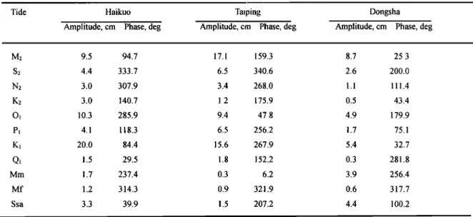
relatively weak in the other SLA series. The amplitudes of the length we used is 1 year. Then the phases and the amplitudes of the components with periods of 173 and 188 days in SLA4 reach 1-2 errors at given tidal frequencies were computed by a least squares

cm and are considered large compared to the same components in harmonic analysis. In general, CSR3.0 has the least error at

the others. These components may well be aliased tidal signals Dongsha, which is surrounded by deep waters. At Haikuo the

arising

from the error of the CSR3.0

tide model

we used

in largest

error

occurs

at K•, while

at Taiping

and

Dongsha

the largest

major ocean tides for T/P, which were computed using [Parke et shelf and has the largest error at K•, the strongest components in al., 1987; Schlax and Chelton, 1994] SLA4 are those with periods of 60-62 days, which we believe are

T(f) =

P

fp- [fp

+ 0.5]

'

(4)

where f is the tidal frequency, p = 9.9156 days is the T/P repeat

period, and [fp + 0.5] is the integer part of OCp +0.5). For T/P the

due to aliased M 2 and S2. Moreover, SLA1 has a relatively strong

173 day component, which becomes smaller in SLA3. SLA3,

being the average of SLA1 and SLA2, contains less tidal aliasing effect because it has no significant components with periods close to the tidal aliasing periods. In practice, if the phase of an aliased tide is spatially smooth, then the tidal aliasing effect may be reduced by averaging SLAs over an area larger than the aliasing periods of the major ocean tides range from 28 to 183 days

and

can

be

mistakenly

associated

with

monthly,

intraseasonal,

and wavelength

of this

aliased

tide.

Formulae

for computing

the

semiannual

sea

level

variability

generated

by wind

and

other

wavelengths

of aliased

tides

are

given

by Schlax

and

Chelton

forcings.

Table

4 shows

the

amplitudes

and

phases

of the

CSR3.0

[1994].

For

example,

the

wavelength

of the

aliased

M2

for

T/P

is

9 ø The widths of the northern SCS and the southern SCS are just tide model errors at Haikuo, Dongsha, and Taiping tide gauge ß

stations,

whose

locations

are given

in Figure

1. To determine

the about

the wavelength

of the aliased

M2, and hence

SLA1

and

CSR3.0

model

error

at a tide

gauge

station,

we first

subtracted

the SLA2

may

marginally

escape

the contamination

of the aliased

M 2

CSR3.0 modeled values from the measured values to get the errors. tide. Because the whole SCS extends more than 9 ø , SLA3 is less

HWANG AND CHEN: FOURIER AND WAVELET ANALYSES OF SOUTH CHINA SEA 28,793

Table 3. Tidal Aliasing Periods of TOPEX/Poseidon for

11 Major Ocean Tides

Tide Aliasing Period, days

M2 62 S2 59 N2 50 K2 87 O2 46 K• 173 Q• 69 Mm 28 Mf 36 Ssa 183

the continental shelf of the SCS is < 9 ø , hence, along with the fact that the M2 error and its phase variation are large, SLA4 contains a

strong component with period equal to the aliasing period of M2.

For comparison, in Figure 6 we show the periodograms of SLA4,

as well as SLA series over the Taiwan Strait, the East China Sea,

and the Yellow Sea, which are all located on the continental shelf

of east Asia. All the SLA series in Figure 6 contain strong

components with periods of about 60 days, which are due to the

aliased M2 and S2 tides. Comparing the periods of the dominant

cmnponents in Figure 6 and the aliasing periods in Table 3, we

believe that the T/P-derived SLAs over the Taiwan Strait and the East China Sea are affected by almost all aliased major ocean tides.

As an example, we find that the Rms difference between CSR3.0

modeled and observed tidal values over 1993-1994 at the Taichung

tide gauge station is 50 cm. The Taichung station is located on the central west coast of Taiwan, and there the tidal amplitude is 3 m.

This explains why SLAs over the Taiwan Strait are so seriously

affected by the aliased tides.

Wind has components with periods of 30-60 days [Philander, 1990], and in particular, the wind over the SCS has a component

lOO

II

- Continental

shelf

of SCS

II - Taiwan Strait

III

,. East

China

Sea

. ]

Yellow

Sea

so 'i

,-

0 2 4 6 8 10 12 14 16 18 20

Frequency (cycle/year)

Figure 6. Comparison of periodograms of TOPEX/Poseidon-derived SLA in four areas of the continental shelf of

28,794 HWANG AND CHEN: FOURIER AND WAVELET ANALYSES OF SOUTH CHINA SEA

with

a period

of 180

days

due

to the

summer

and

winter

monsoons

be easily

used

to identify

the

scale

of the

signal

and

its location

on

(here

we consider

only

the

magnitude

of wind;

see

below).

All the

t axis.

The

constant

1/•a in (5) is to ensure

that

the

norm

of

these wind components may give rise to sea level variability of the

same

frequencies.

Because

of

the

closeness

between

the

periods

of •((t- b)/a) is equal

to the norm

of •(t), i.e.,

the

wind

components

and

the

aliased

periods

of tides,

there

is

The

wavelet

function

•(t) must

have

a

considerable

uncertainty

as to whether

certain

components

in the compact

support

and satisfy

the admissibility

condition,

which

four SLA time series

are due

to aliased

tides

or are due

to wind. demands

that the mean

of •(t) up to a certain

order

of moment

However,

if a component

is due

to an aliased

tide,

then

this be zero.

Furthermore,

small

scale

corresponds

to high

frequency

component

should

show

consistent

amplitude

throughout

the

entire

and large

scale

corresponds

to low frequency.

Thus

C(a,b)

time

span

of a time

series.

To detect

the

time-variation

of the represents

the

time-scale

structure

of a signal.

amplitude of a component will rely on wavelet analysis discussed _{Since data are always given in a discrete form, the continuous}

below. Moreover, to have less tidal aliasing effect and to have a

wavelet transform is approximated as

time series that represents the overall behavior of the SCS sea level,

only

SLA3

will

be

used

in

the

following

analysis.

1 2v-•

nat-

b•,

= • 5• f(nzlt)•( )zlt , (6)

Cj'k

•j .=0

aj

4. Wavelet Analysis of Sea Level Anomaly

In the Fourier

analysis

performed

in Section

3.1, a time

series where

N is the number

of records

and zlt is the sampling

interval.

is regarded as a stationary signal, so that in theory the spectral Equation (6) can be evaluated by algorithms such as fast Fourier content of a segment of the series should be equivalent to that of transform [Totfence and Compo, 1998]. The discrete scales and any other segment. However, many signals, including SLA, are translations are selected as

nonstationary and have time-varying frequencies and amplitudes.

For

example,

sea

level

variabilities

can

be due

to wind,

sea

surface

a• = jAt, j = 2,---,d

max

temperature

(SST),

ENSO,

and

other

forcings

that

have

different bk

= kAt,

k = 0,---,N-1 ,

(7)

magnitudes and frequencies at different times. To see the

time-varying

components

of a signal,

a better

tool

than

Fourier

where

dmax

is a number

<N.

The

indexj

starts

from

2 because

2zlt

analysis

is wavelet

analysis.

In this

study

we employ

both

the is the

smallest

resolvable

scale.

The

choice

of dmax

depends

on

the

continuous

wavelet

transform

and

the

wavelet

multiresolution

spectral

content

of the

analyzed

signal,

[see

also

Torrenee

and

transform

to analyze

SLA and

other

data.

The continuous

Compo,

1998;

Kumar

and

Foufoula-Georgiou,

1994].

Note

that

one-dimensional

wavelet

transform

of a signal,

f(t), is defined

as Torrenee

and

Compo

[1998]

and

Kumar

and

Foufoula-Georgiou

[Daubeehies,

1992]

[1994]

present

two

different

criteria

for

choosing

dmax.

1 Plate l a shows the wavelet coefficients of SLA3 computed

C(a,b)=•aalf(t)•(t-b)dt

_a

,

(5)

with

_1992]

the

real

part

of

the

Morlet

wavelet,

defined

as

[Daubechies,

where

a and

b are

scale

and

translation,

respectively,

•(t) is the

•(t) ----II•-l/4e-t2/2

COS(5t)

,

(8)

wavelet function, and C(a,b) is the wavelet coefficient. If • is a

comr•lex

function,

then

we must

use

the conjugate

of • in (5). The

Morlet

wavelet

is widely

used

in geophysical

research

such

as

Mathematically,

C(a,b)

is

the

projection

off(t)

on

•((t - b)

/ a) or seismic

data

analysis.

Properties

of

the

Morlet

wavelet

in

the

time

similarity

between

f(O and •((t - b) / a), the larger

the coefficient

wavelet

in (8) has

a compact

support

and

satisfies

the

admissibility

C(a,b).

Thus

large

absolute

values

of the wavelet

coefficients

can condition

up to any order

of moment,

see, for example,

the

Table 4. Amplitudes and Phases of CSR3.0 Tide Model Errors :•t Three Tide Gauge Stations of the SCS

Tide Haikuo Taiping Dongsha

Amplitude, cm Phase, deg Amplitude, crn Phase, deg Amplitude, cm Phase, deg

M2 9.5 94.7 17.1 159.3 8.7 25.3 S2 4.4 333.7 6.5 340.6 2.6 200.0 N2 3.0 307.9 3.4 268.0 1.1 111.4 K2 3.0 140.7 1.2 175.9 0.5 43.4 O• 10.3 285.9 9.4 47.8 4.9 179.9 P• 4.1 118.3 6.5 256.2 1.7 75.1 K• 20.0 84.4 15.6 267.9 5.4 32.7 Q• 1.5 29.5 1.8 152.2 0.3 281.8 Mm 1.7 237.4 0.3 6.2 3.9 256.4 Mf 1.2 314.3 0.9 321.9 0.6 317.7 Ssa 3.3 39.9 1.5 207.2 4.4 100.2

HWANG AND CHEN: FOURIER AND WAVELET ANALYSES OF SOUTH CHINA SEA 28,795

Signal

al

a2

a3

a6

dl

d2

d3

d4

d5

d6

d7

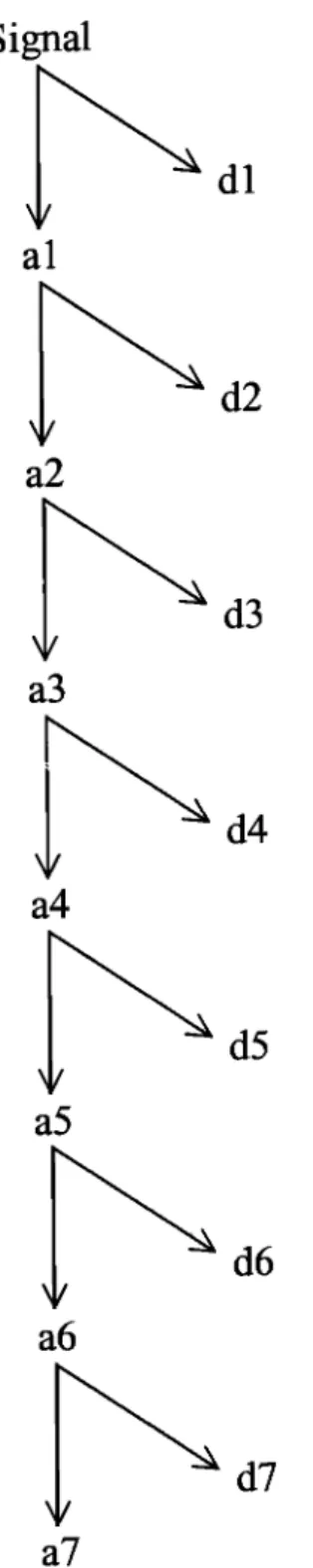
Figure 7. Wavelet decomposition tree of a seven level multi-

resolution wavelet transform.

integration result by Gradshteyn and Ryzhik [1994, p. 531].

According to Torrerice and Compo [ 1998, Table 1 ] the relationship

between the period p (or wavelength) of a Fourier component and

the scale a of the Morlet wavelet given in (8) is

4/ra

p = = 1.232a , (9)

5+42+52

which

helps

to interpret

the wavelet

coefficients

in the Fourier

a zone called "cone of influence (COI)" [Torrence and Compo, 1998] where the coefficients are less reliable than those in other parts of the plot. However, according to Totfence and Compo [1998, p. 67], if the time series is cyclic, there will be no COI. Since the SLA time series (also the time series in Plates lb and lc) is dominated by the annual cycle (see Figure 5) and is almost cyclic, the COI of the wavelet coefficients in Plate 1 should be negligible. Below is a summary of the SLA components identified in Plate 1 a.

1. The 30-120 day components are strong from January 1993 to January 1995 and weak after January 1995. The fact that these components have different amplitudes at different times suggests that SLA3 is not affected by the aliased M2 and S2 tides.

2. The semiannual component is identified as a local high in spring and a local high in winter in each year at period of 6 months. This component is due to the summer and winter monsoons of the SCS. The peaks always occur in May to June (for the spring high) and in November to December (for the winter high). In the springs of 1995 and in the winter of 1997-1998, such semiannual highs

almost disappear. The time-varying amplitude of this component

shows no contamination of aliased K• and Ssa tides in SLA3.

3. The annual component creates the almost periodic wavelet

coefficients that can be easily identified in Plate 1 a. It has a peak in summer, and the time span between two consecutive summer

peaks is about 12 months. The amplitude varies from one year to

another with the largest in 1996 and the smallest in 1994.

4. The wavelet coefficients corresponding to the interannual

components are rather smooth. At periods of 2-3 years, two bands

of highs occur between late 1993 and the summer of 1994 and

between the summer of 1996 and the spring of 1997. Notice that

the two bands of highs occur about 1 year before both the

1994-1995 and the 1997-1998 E1 Nifios. At periods > 3 years, a

band of highs begins in late 1995 and ends in the spring of 1997. In fact, the spring of 1997 is the time when the 1997-1998 E1 Nifio

starts to develop.

Next we perform wavelet multiresolution transform on SLA3.

The multiresolution transform applies a wavelet matrix, consisting

of scaling coefficients, to a data vector hierarchically to obtain a sequence of vectors containing approximations and details at

different levels; see, for example, Press et al. [1993, p. 594] and Chui [1992, p. 20] for the computational algorithm. Thus, with the

wavelet multiresolution transform, a signal is decomposed into

components of different resolutions. For example, Figure 7 shows

the wavelet decomposition tree of a seven-level decomposition of a signal. In Figure 7 we have the relationships a, = a,+•+d,+•, and

signal = a7+d7+do+ds+dg+ds+d2+d•. The higher the degree of

approximation, the lower the resolution. For example, a2 is coarser than a•. This is also true of the details. In this study we used the

scaling coefficients of the Daubechies number 3 (db3) wavelet

[Daubechies, 1992] to form the wavelet matrix for the

multiresolution transform. The db3 wavelet has a compact support

length of five, and up to the third order derivative of its Fourier

transform at the origin (frequency = zero) is zero. Figure 8 shows a

seven-level decomposition of SLA3, which is summarized as

follows.

1. Detail d• detects five anomalously negative SLA values between January 1993 and January 1995. The responsible T/P cycles are 31, 41, 55, 65 and 79, when the Poseidon altimeter was

on. It also shows that between January 1993 and January 1995, the

monthly variability is much stronger than at any other time. 2. Approximations a2 and a3 show the seasonal variations of SLA. Detail d3 shows the almost semiannual variation of sea level

related to the summer and winter monsoons.

3. Approximation

as shows

two local

SLA maxima

in January

1994 and in August

1996,

which

precede

the 1994-1995

and the

transform,

the data

records

were

extended

with

zero

values.

1997-1998

E1

Nifio

and

are

closely

linked

to the

local

highs

in the