國
立
交
通
大
學
電子工程學系 電子研究所碩士班
碩
士
論
文
抵抗簡單能量攻擊法的橢圓曲線運算單元之設計
與實現
Design and Implementation of an SPA-Resistant Dual-Field Elliptic Curve
Arithmetic Unit
研究生:曾知業
指導教授:張錫嘉 教授
抵抗簡單能量攻擊法的橢圓曲線運算單元之設計與實現
Design and Implementation of an SPA-Resistant Dual-Field Elliptic Curve
Arithmetic Unit
研 究 生:曾知業
Student:Chih-Yeh Tseng
指導教授:張錫嘉
Advisor:Hsie-Chia Chang
國 立 交 通 大 學
電 子 工 程 學 系 電 子 研 究 所 碩 士 班
碩 士 論 文
A ThesisSubmitted to Department of Electronics Engineering & Institute of Electronics College of Electrical and Computer Engineering
National Chiao Tung University in Partial Fulfillment of the Requirements
for the Degree of Master In
Electronics Engineering
November 2008
Hsinchu, Taiwan, Republic of China
抵抗簡單能量攻擊法的橢圓曲線運算單元之設計
與實現
學生:曾知業
指導教授
:張錫嘉國立交通大學電子工程學系 電子研究所碩士班
摘
要
這篇論文中介紹了一個同時適用在 GF(p)和 GF(2
m)的抗簡單能量攻擊法
之橢圓曲線運算單元(ECAU)的通用型硬體架構,這個架構能支援最多 512
位元任意長度的有限場。在這個運算單元中提出一種隨機交錯計算 k
1P
1+k
2P
2的演算法,藉此抵抗簡單能量攻擊法。其中的橢圓曲線運算建構在仿射座標
系,並使用高速的蒙哥馬利除法演算法。為了減少硬體複雜度,我們提出了
有限場運算單元(GFAU)來計算同餘加法、減法和蒙哥馬利乘法、除法。
使用 ASIC 設計流程實現這個架構後,GFAU 所需的合成邏輯閘個數比
先人所提出的少 25%。在所提出的抵抗簡單能量攻擊法的 ECAU 中,我們只
運用一套 GFAU,因此合成結果只需 277.K 個邏輯閘。在 133MHz 的時脈下
進行,計算一筆 512 位元的橢圓曲線純量乘法平均需要 13.76ms,而計算一
筆抵抗簡單能量攻擊法的 k
1P
1+k
2P
2運算只需要 27.53ms。
Design and Implementation of an SPA-Resistant Dual-Field Elliptic
Curve Arithmetic Unit
student:Chih-Yeh Tseng
Advisors:Hsie-Chia Chang
Department of Electronics Engineering & Institute of Electronics
National Chiao Tung University
ABSTRACT
A universal hardware architecture of SPA-resistant elliptic curve arithmetic
unit (ECAU) suitable for both GF(p) and GF(2
m) is introduced to work in
arbitrary field lengths within a maximum 512-bit length. The proposed algorithm
used in ECAU can randomly interleave k
1P
1+k
2P
2operations to cope with SPA.
The elliptic curve operations are calculated over affine coordinate using high
speed Montgomery division algorithm. To reduce hardware complexity, the
sharing architecture called Galois field arithmetic unit (GFAU) is proposed to
perform modular addition, modular subtraction, Montgomery multiplication and
Montgomery division.
After implemented by ASIC design flow, the GFAU occupies 25% less
synthesized gatecount than previous work. With only one set of GFAU, the
proposed SPA-resistant ECAU occupies 277.5K gatecount. It averagely takes
13.76ms to perform one 512-bit scalar multiplication and 27.53ms to perform a
SPA-resistant 512-bit k
P
+k
P
operation both at 133MHz clock rate.
誌
謝
說長不長,說短也不短,大約兩年半的研究所生活即將要結束。總結起來,可以說 是既充實又快樂的一段時光。首先,我要感謝指導老師:張錫嘉博士,不但在研究領域上 很有耐心的指引我們,也鼓勵我們嘗試新的思維,給予學生們相當大的空間發揮。生活上 也像是朋友般的關心和照顧,讓實驗室一直保持著和樂融融的氣氛。此外,建青學長帶領 STAR 團隊漸漸的茁壯,研究上遇到許多問題,都是靠學長豐富的經驗才獲得解決,真的 非常感謝。感謝 SECURITY 團隊之前的學長們,尤其是ㄟ羅學長,你的研究論文帶領我進 入橢圓曲線密碼學的世界,給予我非常多的想法,祝你現在工作順利,賺大錢回來請客。 一起努力的 STAR 團隊的成員們,柏均學長統籌研究計畫的大小事,還要幫忙我們解決各 種工具軟體的問題,真的很辛苦;人偉幫忙研究 ECC 的 projective coordinate 給了我不 少非常有用的資訊,最後還得收拾我在計畫的爛攤子,萬分感謝;一起努力的 Q 毛,都靠 你的 word-base 乘法器,計畫才沒有開天窗,也多虧了你帶起的大胃王活動,讓我的肚子 越來越大;廷聿和我們一起討論在能量攻擊法,才能夠領悟到一些原本沒有想到的事情; 其他的學弟們也不斷的替我加油打氣,很感謝你們。此外也感謝 OASIS 實驗室的所有成 員,大頭學長從我剛進實驗室就給我不少指導;國光不厭其煩的替我們解決工作站的問 題,真的很辛苦;修齊也幫我們 review 論文和投影片,當然也幫我搶了不少籃板;永裕、 企鵝、鑫偉都是一起努力拼畢業的夥伴,不但一起寫論文,也一起吃了很多垃圾食物;學 弟妹們也為實驗室帶來許多歡笑,尤其是高手和圓淳,不但在研究上給我不少想法,也是 休閒活動上的好伙伴。還要感謝桑老師的同學和學弟們,尤其是北科第一控衛哲聖,總是 跟我、永裕、鑫偉和圓淳一起奮戰到深夜。 當然,最需要感謝的還是我的家人。很感謝父母給予我的支持和鼓勵,因為你們一 路走來不變的支持和照顧,讓我沒有後顧之憂的完成我的學業,我只有滿心的感謝。遠在 美國的哥哥,你在 MSN 上給我的鼓勵,也讓我感到很窩心,相信你也可以在美國順利的完 成學業。最後還要特別感謝雯怡,研究所兩年多的生活,有妳的陪伴,讓我度過了研究和 生活上的許多挫折。沒有你們就沒有這篇論文,在此再次表達我由衷的感謝。
Design and Implementation of an SPA-Resistant
Dual-Field Elliptic Curve Arithmetic Unit
Student: Chih-Yeh Tseng
Advisor: Dr. Hsie-Chia Chang
Department of Electronics Engineering
National Chiao Tung University
Abstract
A universal hardware architecture of SPA-resistant elliptic curve arithmetic unit (ECAU) suitable for both GF (p) and GF (2m) is introduced to work in arbitrary field lengths within a maximum 512-bit length. The proposed algorithm used in ECAU can randomly inter-leave k1P1+k2P2operations to cope with SPA. The elliptic curve operations are calculated over affine coordinate using high speed Montgomery division algorithm. To reduce hard-ware complexity, the sharing architecture called Galois field arithmetic unit (GFAU) is proposed to perform modular addition, modular subtraction, Montgomery multiplication and Montgomery division.
After implemented by ASIC design flow, the GFAU occupies 25% less synthesized gatecount than previous work. With only one set of GFAU, the proposed SPA-resistant ECAU occupies 277.5K gatecount. It averagely takes 13.76ms to perform one 512-bit scalar multiplication and 27.53ms to perform a SPA-resistant 512-bit k1P1+k2P2 operation both at 133MHz clock rate.
Contents
1 Introduction 1 1.1 Background . . . 1 1.2 Motivation . . . 4 1.3 Thesis Organization . . . 5 2 Elliptic Curves 6 2.1 Basic Facts . . . 72.2 Elliptic Curves Arithmetics over Affine Coordinates . . . 9
2.2.1 Elliptic Curves over the Reals . . . 9
2.2.2 Elliptic Curves over Prime Fields . . . 14
2.2.3 Elliptic Curves over Extension of Binary Fields . . . 14
2.3 Elliptic Curve Arithmetics over Projective Coordinates . . . 16
2.3.1 Homogeneous Projective Coordinates . . . 16
2.3.2 Jacobian Coordinates . . . 17
2.3.3 Chudnovsky-Jacobian Coordinates . . . 18
2.3.4 Modified Jacobian Coordinates . . . 19
2.4 Elliptic Curves Scalar Multiplication . . . 20
2.4.1 Double-and-Add Algorithm . . . 20
2.4.2 Addition-Subtraction Method . . . 21
2.4.3 Binary NAF Method . . . 21
3 Galois Field Arithmetics 23 3.1 Modular Multiplication . . . 23
3.1.1 Traditional Modular Multiplication Algorithm . . . 23
3.1.3 Modified Montgomery Multiplication Algorithm . . . 26
3.1.4 Integer Domain and Montgomery Domain . . . 27
3.2 Modular Inversion . . . 28
3.2.1 Fermat’s Little Theory . . . 28
3.2.2 Extended Euclidean Algorithm . . . 29
3.2.3 Montgomery Modular Inversion Algorithm . . . 33
3.3 Modular Division . . . 35
3.3.1 Multiplication after Inversion . . . 35
3.3.2 Modular Division Algorithm . . . 36
3.3.3 Montgomery Modular Division Algorithm . . . 38
3.4 Domain Transformation . . . 41
3.5 Summary . . . 42
4 Power Analysis 45 4.1 Simple Power Analysis . . . 45
4.2 Differential Power Analysis . . . 47
4.3 Proposed Countermeasures against SPA . . . 49
5 Proposed Architectures 52 5.1 Galois Field Arithmetic Unit . . . 52
5.2 Elliptic Curve Scalar Multiplier . . . 58
5.3 SPA-Resistant Elliptic Curve Arithmetic Unit . . . 61
6 Implementation Results 66 6.1 Design and Test Consideration . . . 66
6.2 Implementation Results and Comparison . . . 67
6.2.1 ASIC Implementation . . . 67
6.2.2 FPGA Implementation . . . 69
List of Figures
1.1 Symmetric-key cryptography block diagram . . . 1
1.2 Asymmetric-key cryptography block diagram . . . 2
2.1 Hierarchal organization of elliptic curve cryptography. . . 6
2.2 Elliptic curves over the reals . . . 10
2.3 Adding two distinct points P + Q = −R . . . 11
2.4 Doubling a point 2P = −R . . . 12
4.1 Interleaved scalar multiplication. . . 51
5.1 Flow chart of the Montgomery division algorithm. . . 53
5.2 Flow chart of the Montgomery multiplication algorithm. . . 55
5.3 Finite states transfer chart of the GFAU. . . 56
5.4 Architecture of the GFAU. . . 57
5.5 State transition chart of the ECSM. . . 59
5.6 Pie graph of the area consumption of the ECSM. . . 60
5.7 Flow chart of the scalar determination scheme. . . 62
5.8 Pie graph of the area consumption of the ECAU. . . 63
5.9 Architecture of the proposed ECSM. . . 64
List of Tables
1.1 Comparable security strength for given cryptography . . . 3
2.1 Point addition formula over reals. . . 14
2.2 Point addition formula over GF (p) . . . 14
2.3 Point addition formula over GF (2m) . . . 15
3.1 Latency of the Montgomery modular inverse from and to both domains. . . 35
3.2 Latency of modular division using traditional method from and to both domain . . . 36
3.3 Latency of Montgomery modular division from and to both domain . . . . 41
3.4 Latency of Montgomery division algorithms comparison. . . 41
3.5 Scalar multiplication comparison between different coordinates. . . 43
3.6 Comparison between different coordinates. . . 44
5.1 Synthesized results for proposed universal dual-field Galois field arithmetic unit on ASIC and FPGA design. . . 58
5.2 Synthesize results for proposed ECSM. . . 61
5.3 Synthesize results for proposed ECAU. . . 63
6.1 ASIC synthesis results comparison . . . 67
6.2 Elliptic Curve Scalar Multiplication ASIC Performance Comparison . . . . 68
6.3 512-bit FPGA synthesis results. . . 69
Chapter 1
Introduction
1.1
Background
The modern cryptography can be roughly split into two kind: symmetric-key tography (secret-key cryptography) and asymmetric-key cryptography (public-key cryp-tography).
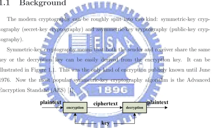
Symmetric-key cryptography means that both the sender and receiver share the same key or the decryption key can be easily derived from the encryption key. It can be illustrated in Figure 1.1. This was the only kind of encryption publicly known until June 1976. Now the most popular symmetric-key cryptography algorithm is the Advanced Encryption Standard (AES) [1].
encryption decryption
plaintext ciphertext plaintext
key
Figure 1.1: Symmetric-key cryptography block diagram
A significant disadvantage of symmetric cryptography is the key management. The sender and the receiver should exchange the same key through a trusted channel. Besides, each distinct pair of communication parties must, ideally, share a different key. The number of keys required increases as the square of the number network members, therefore, complex key management schemes are demanded to keep them all straight and secret.
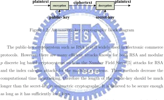
In 1976, Whitfield Diffe and Martin Hellman [2] proposed a novel cryptography called public-key cryptography (also called as asymmetric-key cryptography), which used dis-crete logarithm problem to prevent the secret-key from being acquired with known public-key. It can be illustrated in Figure 1.2. This method of exponential key exchange came to be known as Diffie-Hellman key exchange. RSA and El-Gamal are two of the popu-lar public-key cyrptosystems widely used nowadays. The RSA algorithm based on the difficult of factoring large numbers was published by Rivest, Shamir and Adleman [3] at MIT1 in 1978. Further, the El-Gamal algorithm based on Diffie-Hellman key agreement describes the public-key system and digital signature schemes, and it was proposed by Taher ElGamal [4] in 1985.
encryption decryption
plaintext ciphertext plaintext
public- key secret-key
Figure 1.2: Asymmetric-key cryptography block diagram
The public-key cryptosystem such as RSA is still widely used in electronic commerce protocols. However, there are many efficient attacks known for both RSA and modular p discrete log based cryptosystems such as the Number Field Sieve [5] attacks for RSA and the index calculus attacks for the modular p systems. These methods decrease the computational time in attacking, therefore the length of the public-key should be much longer than the secret-key in symmetric cryptography. It is believed to be secure enough as long as it has sufficiently long keys.
The elliptic curve cryptography (ECC) is kind of public-key cryptography based on the algebraic structure of elliptic curves over finite fields. It was independently proposed by Victor S. Miller of IBM2 in 1986 [6] and Neal Koblitz of the University of Washington in 1987 [7]. There are no subexponential algorithms known for the elliptic curve discrete logarithm problem (ECDLP) and denotes that there are no efficient mathematical attacks known on it. Consequently, the parameters for ECC can be chosen to be much smaller than the parameters for RSA with the same level of resistance against the best known
1
Massachusetts Institute of Technology, located in Cambridge, MA, USA. http://web.mit.edu/
2
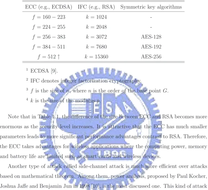
attacks. Table 1.1 shows each different parameter size with the same level of security strengths compared with given cryptography [8].
Table 1.1: Comparable security strength for given cryptography ECC (e.g., ECDSA) IFC (e.g., RSA) Symmetric key algorithms
f = 160 − 223 k = 1024 -f = 224 − 255 k = 2048 -f = 256 − 383 k = 3072 AES-128 f = 384 − 511 k = 7680 AES-192 f = 512 ↑ k = 15360 AES-256 1 ECDSA [9].
2 IFC denotes integer factorization cryptography.
3 f is the size of n, where n is the order of the base point G. 4 k is the size of the modulus p.
Note that in Table 1.1, the difference of the size between ECC and RSA becomes more enormous as the security level increases. It is attractive that the ECC has much smaller parameters leads to more significant performance advantages contrast to RSA. Therefore, the ECC takes advantages for wireless applications where the computing power, memory and battery life are limited such as smart cards and wireless devices.
Another type of attack called side-channel attack is much more efficient over attacks based on mathematical theorem. Among them, power analysis, proposed by Paul Kocher, Joshua Jaffe and Benjamin Jun in 1998 [10], is the most discussed one. This kind of attack can extract cryptographic keys and other secret information from the device without invasion. It works over all kinds of public-key and secret-key cyrptosystems. Most of all, it’s the only efficient attack on elliptic curve cryptosystem. Lots of countermeasures were proposed to resist power analysis. To learn more information about the countermeasures, [11] can be referred. A detailed introduction of power analysis attack will be given in chapter 4.
Furthermore, the performance of ECC mainly depends on the efficiency of its modular arithmetics, namely, scalar multiplication. Given a positive integer, and a point P on an
elliptic curve. The scalar multiplication kP can easily be computed by iterative additions and doublings. There are some algorithms to compute the multiple of points on elliptic curves. More details will be discussed in chapter 2.4 later.
1.2
Motivation
The scalar multiplication is the most important operation in an elliptic curve cryp-tosystem due to the ECDLP. In the traditional affine coordinate elliptic curve point representation, the result of addition and doubling can be derived through several mod-ular multiplication and one modmod-ular division. Modmod-ular multiplication has been improved by the Montgomery’s technique [12] which will be discussed in chapter 3.1.2. Tradition-ally, modular division can be achieved by modular multiplication after modular inversion. Then modular inversion can be done by iterative modular multiplication introduced in the Fermat’s little theorem or by iterative modular addition, subtraction and shifting intro-duced by extended Euclidean algorithm. But the first one is extremely time-consuming and the second one is area-consuming.
Elliptic curve is not only presented in general affine coordinates, it has some different projective coordinates representations. Equations in elliptic curve scalar multiplication only consists of modular addition and modular multiplication. Though more multiplica-tions are utilized, it only requires one modular multiplier. Therefore, most research in recent years focus on the optimization on the Montgomery multiplication algorithm.
The modular division is further improved and modified with the Montgomery tech-nique by Yao-Jen Liu in 2007 [13]. In his design, existing inversion after multiplication algorithm is replaced by just one Montgomery division. Hence the area and the compu-tational time is reduced, which will be discussed in chapter 3.3.
Therefore, in this thesis, an approach is provided to compute the scalar multiplication on elliptic curves in both GF (p) and GF (2m), and a unified Montgomery multiplication and division design is proposed to deal with various finite field degrees and different primitive polynomials in GF (2m). In this way, performance in terms of the area by computational time is near to that of projective coordinates algorithms. Therefore affine coordinates algorithms can be bring back to compete with projective coordinates ones.
1.3
Thesis Organization
In this thesis, a universal dual-field elliptic curve arithmetic unit is proposed. In Chapter 2, the preliminary mathematical background of elliptic curves is introduced. In Chapter 3, the Galois field arithmetics is introduced. The Montgomery technique is also involved to improve the multiplication and the division. In Chapter 4, the power analysis attack and its countermeasures are introduced. In Chapter 5, all the proposed universal dual-field architectures are described. In Chapter 6, it shows the hardware implementation results and test consideration. The conclusion is given in Chapter 7.
Chapter 2
Elliptic Curves
ECDH, ECDSA, ECIES
Elliptic Curve Doubling, Addition, Scalar Multiplication, Hash Functions
Galois Field Arithmetics
Complex operations Fundamental arithmetics
Cryptographic protocols
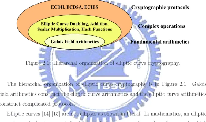
Figure 2.1: Hierarchal organization of elliptic curve cryptography.
The hierarchal organization of elliptic curve cryptography is in Figure 2.1. Galois field arithmetics construct the elliptic curve arithmetics and the elliptic curve arithmetics construct complicated protocols.
Elliptic curves [14] [15] are not ellipses as shown in literal. In mathematics, an elliptic curve is an algebraic curve defined by a cubic equation such as y2 = x3 + ax + b, which is non-singular, i.e. its graph has no cusps or self-intersections. Elliptic curves received their name from their relation to elliptic integrals such as
Z z2 z1 dx √ x3+ ax + b and Z z2 z1 x dx √ x3+ ax + b (2.1)
2.1
Basic Facts
Let F be an algebraically closed field and F2denote the affine plane A2, the usual plane, A2(F) = {(x, y)|x, y ∈ F}. Let C(x, y) be an irreducible polynomial over F, and the curve C means the set of zeros of C in the affine plane F2, i.e. {(x, y) ∈ F2|C(x, y) = 0}. Assume that P is a point (xp, yp) on the curve C. If both of the partial derivatives vanish at P , that is ∂C(xp,yp)
∂x =
∂C(xp,yp)
∂y = 0, then the point P is called a singular point on the curve C. A curve is called a singular curve if and only if it has at least one singular point on it, otherwise it is called a non-singular curve. An elliptic curve commonly used in cryptography is a non-singular curve because of its better security level relative to a singular curve. A singular elliptic curve is thought of insecure in general. Definition 2.1 shows the algebraic equation of the elliptic curve in a more general form.
Definition 2.1. An elliptic curve E over the field F defined by an affine Weierstrass equation is an equation of the form
Y2+ a1XY + a3Y = X3+ a2X2+ a4X + a6, ∀ai ∈ F (2.2) let E(F) denote the elliptic curve E over F, i.e. the set of points (x, y) ∈ F2 that satisfy this equation, along with the point at infinity denoted by O.
Definition 2.2. The point at infinity called O is the intersection of the y-axis and the line at infinity. The line at infinity is the set of points on the projective plane for which Z = 0. Therefore, the point at infinity O is (0, 1, 0) in the projective plane, i.e. the equivalence class with X = Z = 0.
No further details about projective plane are shown in this thesis since only affine coordinates are discussed in the remaining chapters.
In order to describe a singular or non-singular curve clearly, an important quantity ∆ related to the elliptic curve called the discriminant of E is defined.
Definition 2.3. ∆ is the discriminant of E and is given by ∆ = −b22b8− 8b34− 27b26+ 9b2b4b6, where b2 = a21+ 4a2 b4 = 2a4+ a1a3 b6 = a23+ 4a6 b8 = a21a6+ 4a2a6 − a1a3a4 +a2a23− a24 (2.3)
and the symbols above correspond to (2.2).
Theorem 2.1. A cubic curve defined by a Weierstrass equation (2.2) is singular if and only if its discriminant ∆ is zero.
The Definition 2.1 is feasible for any field F. However, the elliptic curves commonly used in cryptography are over the finite field GF (q), where q is either a large prime p or a power of p. If q is a large prime p, the prime field GF (p), also labeled as Fp or Zp, is a field of characteristic p where p 6= 2, 3, that is, Pk
i=11 = k 6= 0 for 1 ≤ k < p and Pp
i=11 = 0. If q is a power of p, denoted by pm, the Galois field GF (pm) is an extension field of GF (p), where p is typically chosen as 2 for the sake of binary property in hardware. The finite fields are also called Galois fields, in honor of their discoverer.
On the basis of various characteristics, the Weierstrass equation (2.2) can be simplified into different forms by a linear change of variables. The following paragraphs shows the equation for a field of characteristic 6= 2, 3 and a field of characteristic 2.
Let F be a field of characteristic 6= 2, 3 and char(F) denote the characteristic of F. Since the char(F) 6= 2, substitute (X, Y ) by (X, Y −a1X+a3
2 ) on the left hand side in (2.2). Y2+ a1XY + a3Y substitute (X, Y ) → (X, Y − a1X + a3 2 ) ⇒ (Y −a1X+a3 2 )2+ a1X(Y − a1X+a3 2 ) + a3(Y − a1X+a3 2 ) = Y2−a2 1 4X 2− a1a3 2 X − a2 3 4 (2.4)
Notice that both XY and Y term are eliminated so the coefficients a1 and a3 should be zero. Thus the equation (2.4) results in Y2 by substitution for a
1 = a3 = 0. Further, the char(F) 6= 3 so substitute (X, Y ) by (X −a2
3 , Y ) on the right hand side in equation (2.2). X3+ a2X2+ a4X + a6 substitute (X, Y ) → (X − a2 3 , Y ) ⇒ (X −a2 3 ) 3+ a 2(X −a32)2+ a4(X −a32) + a6 = X3+ (−1 3 a 2 2+ a4)X + (272 a32− 13a2a4+ a6) (2.5)
Then again, the X2 term is eliminated so that the coefficient a
2 should be zero and the equation (2.5) results in X3+ a
4X + a6 by setting a2 = 0. According to (2.4) and (2.5), let a1 = a2 = a3 = 0, a4 = a, a6 = b and the equation (2.2) is modified as follows
Y2 = X3+ aX + b, a, b ∈ F (2.6)
where char(F) 6= 2, 3. Note that the elliptic curve is a smooth curve, i.e. the curve is non-singular. Review in Theorem (2.1), an elliptic curve should have its discriminant nonzero. Therefore, the discriminant of the cubic curve (2.6) can be derived through (2.3) by substitution for a1 = a2 = a3 = 0, a4 = a, a6 = b. Thus ∆ = −16(4a3+ 27b2) 6= 0.
For a field of characteristic 2, only the non-supersingular case is considered. In brief, non-supersingular has the result of the coefficient a1 6= 0. Since a1 6= 0, substitute (X, Y ) by (a2 1X +a 3 a1, a 3 1Y + a2 1a4+a23 a3
1 ) in (2.2) likewise. A simplified form is obtained as follows
Y2+ XY = X3+ aX2+ b, a, b ∈ F (2.7)
where char(F) = 2. There is no need to care whether or not the cubic polynomial on the right hand side in (2.7) has multiple roots.
2.2
Elliptic Curves Arithmetics over Affine
Coordi-nates
Elliptic curve cryptography makes use of elliptic curves where the variables and co-efficients are belong to a finite field. Two kinds of elliptic curves are commonly used in cryptographic applications. They are prime curves over GF (p) and binary curves over GF (2m) respectively. Before discussion on the above curves, the elliptic curves over the reals are first introduced because some of the basic concepts are easier to visualize.
2.2.1
Elliptic Curves over the Reals
According to equation (2.6), a definition for elliptic curves over the reals is given below. Definition 2.4. A non-singular elliptic curve E over the reals is an equation of the form
y2 = x3+ ax + b (2.8)
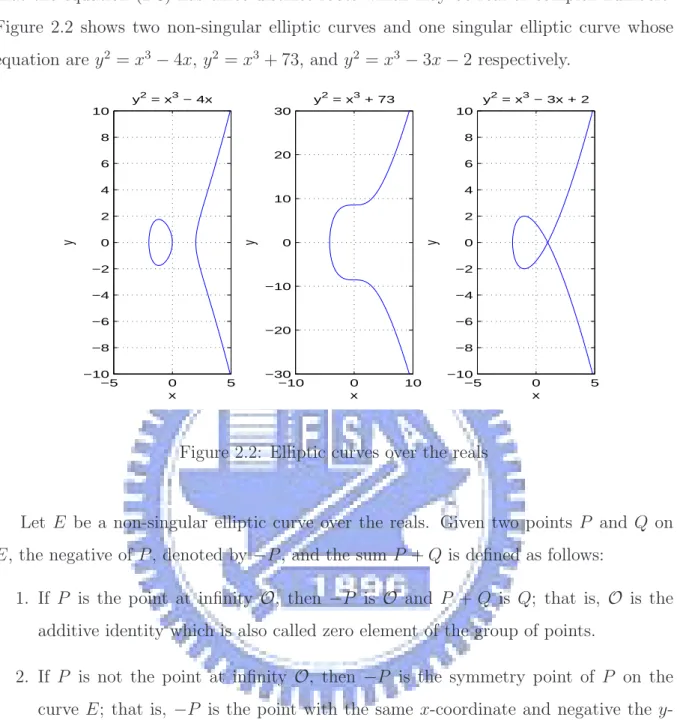
It can be shown that the condition 4a3+ 27b2 6= 0 is necessary and sufficient to ensure that the equation (2.8) has three distinct roots which may be real or complex numbers. Figure 2.2 shows two non-singular elliptic curves and one singular elliptic curve whose equation are y2 = x3− 4x, y2 = x3+ 73, and y2 = x3− 3x − 2 respectively.
−5 0 5 −10 −8 −6 −4 −2 0 2 4 6 8 10 x y y2 = x3 − 4x −10 0 10 −30 −20 −10 0 10 20 30 x y y2 = x3 + 73 −5 0 5 −10 −8 −6 −4 −2 0 2 4 6 8 10 x y y2 = x3 − 3x + 2
Figure 2.2: Elliptic curves over the reals
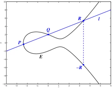
Let E be a non-singular elliptic curve over the reals. Given two points P and Q on E, the negative of P , denoted by −P , and the sum P + Q is defined as follows:
1. If P is the point at infinity O, then −P is O and P + Q is Q; that is, O is the additive identity which is also called zero element of the group of points.
2. If P is not the point at infinity O, then −P is the symmetry point of P on the curve E; that is, −P is the point with the same x-coordinate and negative the y-coordinate of P , i.e. −(x, y) = (x, −y). According to equation (2.8), if (x, y) is a point on the curve E, then the point (x, −y) is consequently on the curve E. 3. If P and Q are different points on E with different x-coordinates, then let l be the
line through P and Q, and the line l intersects the curve E in exactly one more point R. Then the sum P + Q = −R is defined and is illustrated in Figure 2.3. 4. If P and Q are different points on E with the same x-coordinates, that is, Q is a
−4 −3 −2 −1 0 1 2 3 4 5 6 −10 −8 −6 −4 −2 0 2 4 6 8 10 x y P Q R −R l E
Figure 2.3: Adding two distinct points P + Q = −R
5. If P and Q are the same points on E, then let the line l be the tangent line to the curve at P and the point R be the only other point of intersection of l with the curve E. Thus the sum P + Q = P + P = 2P = −R is defined and is illustrated in Figure 2.4. Furthermore, if the tangent line has a double tangency at P , that is, P is a point of inflection, then the sum P + Q = P + P = 2P = −P is defined. In figure 2.3, let (x1, y1), (x2, y2), (x3, −y3) and (x3, y3) denote the coordinates of P , Q, R and P + Q respectively. Let l : y = λx + β be the equation of the line through P and Q then λ = y2−y1
x2−x1 is the slope of the line l and β = y1− λx1 = y2− λx2 is the consequence
of the point P lying on the line l. Assume that t is a variable and (t, λt + β) denotes the coordinates of arbitrary points on the line l. The point on l simultaneously lies on the elliptic curve E if and only if (t, λt+β) satisfies equation (2.8) so that (λt+β)2 = t3+at+b and rearrange it below by order of t.
t3+ (−λ2)t2+ (a − 2λβ)t + (b − β2) = 0 (2.9) Note that the equation has exactly three distinct roots and two of them are known as x1 and x2. Remember the relation between roots and coefficient mentioned in Vi´ete formula first proposed by Fran¸cois Vi´ete (1540–1603), a French mathematician.
−4 −3 −2 −1 0 1 2 3 4 5 6 −10 −8 −6 −4 −2 0 2 4 6 8 10 x y P R l −R E
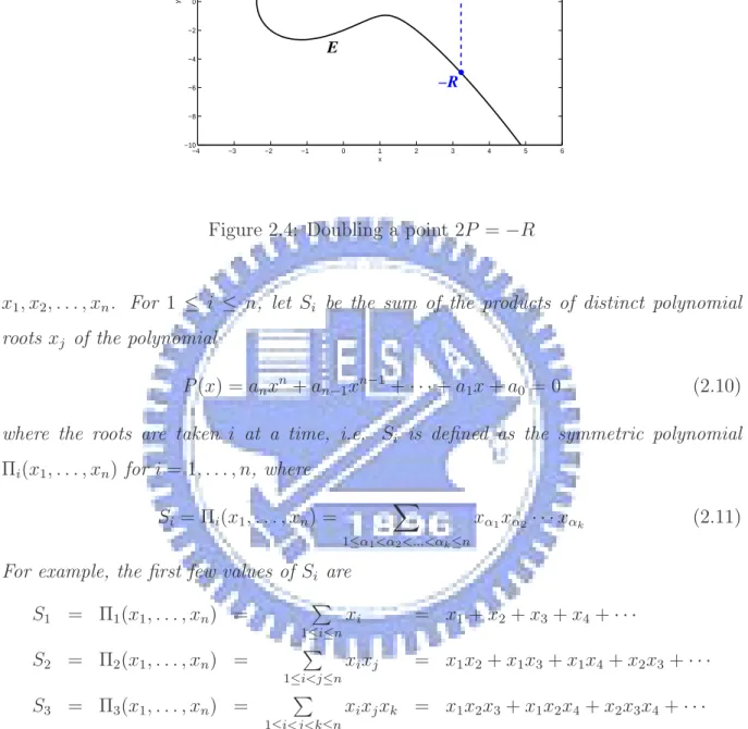
Figure 2.4: Doubling a point 2P = −R
x1, x2, . . . , xn. For 1 ≤ i ≤ n, let Si be the sum of the products of distinct polynomial roots xj of the polynomial
P (x) = anxn+ an−1xn−1+ · · · + a1x + a0 = 0 (2.10) where the roots are taken i at a time, i.e. Si is defined as the symmetric polynomial Πi(x1, . . . , xn) for i = 1, . . . , n, where
Si = Πi(x1, . . . , xn) =
X
1≤α1<α2<...<αk≤n
xα1xα2· · · xαk (2.11)
For example, the first few values of Si are S1 = Π1(x1, . . . , xn) = P 1≤i≤n xi = x1+ x2+ x3+ x4+ · · · S2 = Π2(x1, . . . , xn) = P 1≤i<j≤n xixj = x1x2+ x1x3+ x1x4+ x2x3+ · · · S3 = Π3(x1, . . . , xn) = P 1≤i<j<k≤n xixjxk = x1x2x3+ x1x2x4+ x2x3x4+ · · · and so on. Then Vi´ete’s formula states that
Si = (−1)i an−i
an
(2.12) Proof. The polynomial P (x) can also be written as
P (x) = an(x − x1)(x − x2) · · · (x − xn)
= an(xn− S1xn−1 + S2xn−2− · · · + (−1)nSn)
According to equation (2.10), setting the coefficients equal yields an(−1)iSi = an−i
which is what the Vi´ete’s formula states for. Q.E.D.
The Vi´ete formula was proved by Vi´ete (1579) for positive roots only, and the general theorem was proved by G´erard Desargues (1591–1661). Therefore the sum of the roots s1 of a monic polynomial shown in (2.9) is equal to minus the coefficient of the second-to-highest order. A monic polynomial or normed polynomial is a polynomial whose leading coefficient is equal to 1. It concludes that the third root x3 in (2.9) is equal to λ2− x1− x2 since the sum of the three distinct roots s1 is λ2. Then the y-coordinate of R is λx3 + β and y3 is minus the y-coordinate of R. Therefore the coordinate of P + Q in terms of x1, x2, y1, y2 is shown below. x3 = ( y2− y1 x2− x1 )2− x1− x2 y3 = ( y2− y1 x2− x1 )(x1− x3) − y1 (2.14)
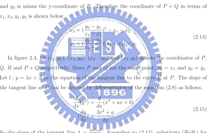
In figure 2.4, let (x1, y1), (x2, y2), (x3, −y3) and (x3, y3) denote the coordinates of P , Q, R and P + Q respectively. Since P and Q are the same point, x2 = x1 and y2 = y1. Let l : y = λx + β be the equation of the tangent line to the curve E at P . The slope of the tangent line at P can be derived by differentiation of the equation (2.8) as follows.
d dx(y 2) = d dx(x 3+ ax + b) (dy dx) = 3x2+ a 2y (2.15)
So the slope of the tangent line λ = 3x21+a
2y1 . According to (2.14), substitute (
y2−y1
x2−x1) for
(3x21+a
2y1 ) and x2 = x1, y2 = y1. A formula for doubling a point is obtained.
x3 = ( 3x2 1+ a 2y1 )2− 2x1 y3 = ( 3x2 1+ a 2y1 )(x1− x3) − y1 (2.16)
Point Addition (P 6= Q) Point Doubling (P = Q) P + Q x3 = λ2− x1− x2 y3 = λ(x1− x3) − y1 λ = y2−y1 x2−x1 x3 = λ2− 2x1 y3 = λ(x1− x3) − y1 λ = 3x21+a 2y1
Table 2.1: Point addition formula over reals.
2.2.2
Elliptic Curves over Prime Fields
Let p > 3 be a prime. Elliptic curves over GF (p) are defined almost the same as they are over the reals and the operations over the reals are replaced by modulus operations. Definition 2.5. Let p > 3 be a prime. A non-singular elliptic curve E over the finite field GF (p) is an equation of the form
y2 ≡ x3+ ax + b (mod p) (2.17)
where a, b ∈ GF (p) are constants such that 4a3+ 27b2 6≡ 0 (mod p).
Assume that (x1, y1), (x2, y2) and (x3, y3) denote the coordinates of P , Q and P + Q respectively. Then the coordinate of −P is defined as (x1, −y1) and P + (−P ) = O. According to equation (2.14) and (2.16), the point addition formula of the elliptic curves over GF (p) is shown in Table 2.2.
Point Addition (P 6= Q) Point Doubling (P = Q) P + Q x3 ≡ λ2 − x1 − x2 (mod p) y3 ≡ λ(x1− x3) − y1 (mod p) λ ≡ y2−y1 x2−x1 (mod p) x3 ≡ λ2− 2x1 (mod p) y3 ≡ λ(x1 − x3) − y1 (mod p) λ ≡ 3x 2 1+a 2y1 (mod p)
Table 2.2: Point addition formula over GF (p)
2.2.3
Elliptic Curves over Extension of Binary Fields
Definition 2.6. Let p(x) be a primitive polynomial of degree m. A non-supersingular elliptic curve E over the extension of binary field GF (2m) is an equation of the form
y2+ xy = x3 + ax2+ b (2.18)
Note that in this subsection, all of the arithmetic operations are defined over GF (2m) and all of the parameters are belong to GF (2m), too. Assume that (x
1, y1), (x2, y2) and (x3, y3) denote the coordinates of P , Q and P + Q respectively. Then the coordinate of −P is defined as (x1, x1+ y1) and P + (−P ) = O.
If P 6= Q, let l : y = λx+β be the equation of the line through P and Q then λ = y2+y1
x2+x1
is the slope of the line l and β = y1+ λx1 = y2+ λx2 is the consequence. The following equation shows all of the points (t, λx + β) on l simultaneously lies on the curve E.
t3+ (λ2+ λ + a)t + (β2+ b) = 0 (2.19)
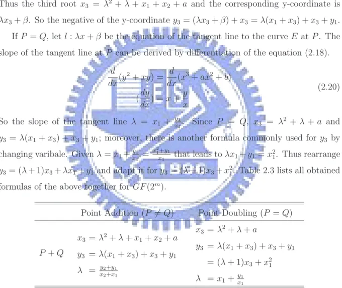
Thus the third root x3 = λ2 + λ + x1 + x2 + a and the corresponding y-coordinate is λx3+ β. So the negative of the y-coordinate y3 = (λx3+ β) + x3 = λ(x1+ x3) + x3+ y1. If P = Q, let l : λx + β be the equation of the tangent line to the curve E at P . The slope of the tangent line at P can be derived by differentiation of the equation (2.18).
d dx(y 2+ xy) = d dx(x 3+ ax2+ b) (dy dx) = x + y x (2.20)
So the slope of the tangent line λ = x1 + xy11. Since P = Q, x3 = λ
2 + λ + a and y3 = λ(x1 + x3) + x3 + y1; moreover, there is another formula commonly used for y3 by changing varibale. Given λ = x1+xy11 =
x2 1+y1
x1 that leads to λx1+ y1 = x
2
1. Thus rearrange y3 = (λ + 1)x3+ λx1+ y1 and adapt it for y3 = (λ + 1)x3+ x21. Table 2.3 lists all obtained formulas of the above together for GF (2m).
Point Addition (P 6= Q) Point Doubling (P = Q)
P + Q x3 = λ2+ λ + x1+ x2+ a y3 = λ(x1+ x3) + x3+ y1 λ = y2+y1 x2+x1 x3 = λ2+ λ + a y3 = λ(x1+ x3) + x3+ y1 = (λ + 1)x3+ x21 λ = x1+ yx11
2.3
Elliptic Curve Arithmetics over Projective
Coor-dinates
Traditionally, the Galois field inversion is accomplished using the Fermat’s little the-orem described in chapter 3.2.1 which is estimated to take 9 to 30 Galois field multipli-cation’s computational time in case of GF (p) with p larger than 100 bits [16]. Therefore, transferring the point coordinates into another coordinates that can eliminate the inver-sion operation can greatly improve the performance.
Except Affine coordinate, there are four different coordinate systems mentioned in this section: Homogeneous Projective, Jacobian, Chudnovsky-Jacobian and Modified Ja-cobian. The computational time is represented in terms of number of multiplications (M) and squaring (S). For simplicity, the addition, subtraction and multiplication by a small constant will not be taken into consideration because they are very fast compared to multiplication, squaring and inversion operations. A comparison table including Affine coordinate is given at chapter 3.5 in Table 3.6. Note that the equations mentioned in the following sections are all used over prime field since the prime field operation is the main concern in this thesis.
2.3.1
Homogeneous Projective Coordinates
In the homogeneous projective coordinates the following transformation functions are used to substitute x and y in the affine Weierstrass equation in equation 2.2 to get the projected coordinates: ( x → X Z y → Y Z (2.21) The elliptic curve equation becomes:
Y2Z = X3+ aXZ2+ bZ3 (2.22)
In this coordinate system, the points P, Q and R are represented as follows: P = (X1, Y1, Z1), Q = (X2, Y2, Z2) and R = P + Q = (X3, Y3, Z3).
• The addition formulas are given by:
where:
u = Y2Z1− Y1Z2, v = X2Z1− X1Z2 and A = u2Z1Z2− v3− 2v2X1Z2
• The doubling formulas are given by (R = 2P ): X3 = 2hs, Y3 = w(4B − h) − 8Y12s2, Z3 = 8s3 where:
w = aZ2
1 + 3X12, s = Y1Z1, B = X1Y1s and h = w2− 8B
The computational time for addition and doubling operations using homogeneous coor-dinates is (12M+2S) and (7M+5S) respectively.
2.3.2
Jacobian Coordinates
In the Jacobian coordinates the following transformation functions are used: ( x → X
Z2
y → Y Z3
(2.23) The elliptic curve equation becomes:
Y2 = X3+ aXZ4+ bZ6 (2.24)
In this coordinate system, the points P, Q and R are represented as follows: P = (X1, Y1, Z1), Q = (X2, Y2, Z2) and R = P + Q = (X3, Y3, Z3).
• The addition formulas are given by:
X3 = −H3− 2U1H2+ r2, Y3 = −S1H3 + r(U1H2− X3), Z3 = Z1Z2H where:
U1 = X1Z22, U2 = X2Z12, S1 = Y1Z23, S2 = Y2Z13, H = U2− U1 and r = S2− S1
• The doubling formulas are given by (R = 2P ): X3 = T , Y3 = −8Y14+ M (S − T ), Z3 = 2Y1Z1 where:
The computational time for addition and doubling operations using Jacobian coordinates is (12M+4S) and (4M+6S) respectively.
2.3.3
Chudnovsky-Jacobian Coordinates
D. V. Chudnovsky [17] concluded that Jacobian coordinate system provide faster dou-bling and slower addition compared to projective coordinates. In order to speedup ad-dition, he proposed the Chudnovsky-Jacobian coordinate system.In this coordinates a Jacobian coordinates point is represented internally as 5-tupel point (X, Y, Z, Z2, Z3). The transformation and elliptic curve equations are the same as in Jacobian coordinates, while the points P, Q, and R represented as follows: In this coordinate system, the points P, Q and R are represented as follows:
P = (X1, Y1, Z1, Z12Z13), Q = (X2, Y2, Z2, Z22, Z23) and R = P +Q = (X3, Y3, Z3, Z32, Z33). The main idea in Chudnovsky-Jacobian coordinate is that the Z2, Z3 are already calculated in the previous iteration and are not necessary to be calculated again in the current iteration. In other words, Z2
1, Z13, Z22, Z23 are computed during the previous iteration and fed into the current iteration as inputs, while Z2
3, Z33 need to be calculated. • The addition formulas are given by:
X3 = −H3 − 2U1H2 + r2, Y3 = −S1H3 + r(U1H2 − X3), Z3 = Z1Z2H, Z32 = Z32, Z3
3 = Z33 where:
U1 = X1Z22, U2 = X2Z12, S1 = Y1Z23, S2 = Y2Z13, H = U2− U1 and r = S2− S1
• The doubling formulas are given by (R = 2P ):
X3 = T , Y3 = −8Y14+ M (S − T ), Z3 = 2Y1Z1, Z32 = Z32, Z33 = Z33 where:
S = 4X1Y12, M = 3X12+ aZ14, and T = −2S + M2
The computational time for addition and doubling operations using Chudnovsky-Jaconian coordinates is (11M+3S) and (5M+6S) respectively.
2.3.4
Modified Jacobian Coordinates
Henri Cohen et.al. modified the Jacobian coordinates [16] and claimed that they got the fastest possible point doubling. The term (aZ4) is needed in doubling rather than in addition. Taking this into consideration, they employed the idea of internally representing this term and provide it as input to the doubling formula. The point is represented in 4-tuple representation (X, Y, Z, aZ4). It uses the same transformation equations used in Jacobian coordinates.
In this coordinate system, the points P, Q and R are represented as follows: P = (X1, Y1, Z1, aZ14), Q = (X2, Y2, Z2, aZ24) and R = P + Q = (X3, Y3, Z3, aZ34).
• The addition formulas are given by:
X3 = −H3− 2U1H2+ r2, Y3 = −S1H3 + r(U1H2− X3), Z3 = Z1Z2H, aZ34 = aZ34 where:
U1 = X1Z22, U2 = X2Z12, S1 = Y1Z23, S2 = Y2Z13, H = U2− U1 and r = S2− S1
• The doubling formulas are given by (R = 2P ):
X3 = T , Y3 = M (S − T ) − U, Z3 = 2Y1Z1, aZ34 = 2U (aZ14) where:
S = 4X1Y12, U = 8Y14, M = 3X12+ aZ14, and T = −2S + M2
The computational time for addition and doubling operations using Modified Jacobian coordinates is (13M+6S) and (4M+4S) respectively.
2.4
Elliptic Curves Scalar Multiplication
Scalar multiplication is used to compute a multiple of an Elliptic curve point kP , where P is an elliptic curve point and k is a positive integer except the condition that k equals to the order of P , then kP is the point obtained by adding together k copies of P and this operation dominates the execution time of elliptic curve cryptographic schemes.
2.4.1
Double-and-Add Algorithm
Algorithm 2.1. (Left-Right Double-and-Add Algorithm)
Input: A positive integer k < n, where n is the order of P ; and an elliptic curve point P . Output: The elliptic curve point kP .
1. Let knkn−1. . . k1k0 be the binary representation of k, where the leftmost bit kn is 1. 2. Set R = P .
3. For i from n − 1 down to 0 do 3.1 Set R = 2R.
3.2 If ki = 1, then set R = R + P . 4. Output R.
Algorithm 2.2. (Right-Left Double-and-Add Algorithm)
Input: A positive integer k < n, where n is the order of P ; and an elliptic curve point P . Output: The elliptic curve point kP .
1. Let knkn−1. . . k1k0 be the binary representation of k, where the leftmost bit kn is 1. 2. Set R = inf inity, Q = P .
3. For i from 0 down to n − 1 do 3.1 If ki = 1, then set R = R + Q. 3.2 Set Q = 2Q.
4. Output R.
The double-and-add algorithm is a basic method for calculating scalar multiplication. It achieves by repeated point double and add operations. The expected number of ones in the binary representation of k is m
2, where m is the length of the integer k. The number of ones in k indicates the number of times that point addition performs and the number of times that point doubling operation performs is approximately equal to m.
Thus Algorithm 2.1 averagely takes m2 times point addition and m times point doubling to perform m-bit elliptic curve scalar multiplication once.
Algorithm 2.2 calculates the scalar multiplication in an opposite way. It also achieves by repeated point double and add operations. But if there exist one doubling hardware and one addition hardware, it can achieve the double and add operations simultaneously. It is useful in DPA resistant mentioned later in chapter 4.
2.4.2
Addition-Subtraction Method
If P (x, y) ∈ E(Fp) then −P = (x, −y); else if P (x, y) ∈ E(F2m) then −P = (x, x + y).
Thus the point subtraction is as efficient as point addition. Then Algorithm 2.1 is replaced by using addition-subtraction method and shown in Algorithm 2.3.
Algorithm 2.3. (Addition-Subtraction Method)
Input: A positive integer k < n, where n is the order of P ; and an elliptic curve point P . Output: The elliptic curve point kP .
1. Let enen−1. . . e1e0 be the binary representation of 3k, where the leftmost bit en is 1. 2. Let knkn−1. . . k1k0 be the binary representation of k.
3. Set R = P .
4. For i from n − 1 down to 1 do 4.1 Set R = 2R.
4.2 If ei = 1 and ki = 0, then set R = R + P . 4.3 If ei = 0 and ki = 1, then set R = R − P . 5. Output R.
2.4.3
Binary NAF Method
Owing to point subtraction is as efficient as point addition, the signed digit representa-tion k =P ki2iis used, where ki ∈ {0, ±1}. A non-adjacent form (NAF) is a useful signed representation which has the property that no two consecutive bits in k are nonzero and has the fewest nonzero bits of any signed digit representation of k. Each positive integer k has its unique NAF, denoted by NAF(k). The NAF of an integer k can be computed efficiently by using Algorithm 2.4 [18].
Algorithm 2.4. (NAF of a Positive Integer) Input: A positive integer k.
Output: NAF(k). 1. Set i = 0. 2. While k ≥ 1 do
2.1 If k is odd, then set ki = 2 − (k mod 4) and then set k = k − ki; else set ki = 0. 2.2 Set k = k
2 and i = i + 1.
3. Output k, whose binary representation is (ki−1ki−2. . . k1k0).
Note that the length of NAF(k) is at most one bit longer than the binary representation of k and the average density of nonzero bits in NAF(k) is approximately m
3 [19], where m is the length of the integer k.
Algorithm 2.5. (Binary NAF Method) Input: NAF(k) and an elliptic curve point P . Output: The elliptic curve point kP .
1. Let knkn−1. . . k1k0 be signed digit representation of k, where the leftmost bit kn is 1. 2. Set R = P .
3. For i from n − 1 down to 0 do 3.1 Set R = 2R.
3.2 If ki = 1, then set R = R + P . 3.3 If ki = −1, then set R = R − P . 4. Output R.
Then the Algorithm 2.5 modifies Algorithm 2.1 by using NAF(k) instead of the binary representation of k and averagely takes approximately m
3 times point addition and m times point doubling to perform m-bit elliptic curve scalar multiplication once. Furthermore, it follows that the expected running time of Algorithm 2.3 and Algorithm 2.5 are the same.
Chapter 3
Galois Field Arithmetics
In abstract algebra, Galois field, named in honor of ´Evariste Galois(1811–1832), which has the same meaning with finite fields is a field that contains only finitely many elements. It plays an important role in number theory, algebraic theory, Galois theory, coding theory, and cryptography. In an elliptic curve cryptosystem, Galois field arithmetics occupy almost all computation time. Therefore, the most efficient method to improve the performance of the entire cryptosystem is to optimize the algorithms for the Galois field arithmetics.
A thorough introduction to GF (p) and GF (2m) can be found in publications about abstract algebra. To understand the basic mathematical background required in cryp-tography, Chapter II in [14] written by Neal Kobitz can be referred. In this chapter, algorithms for modular multiplication, inversion, and division are respectively introduced in section 3.1, 3.2, and 3.3. Domain transformation illustrated in section 3.4, and perfor-mance comparison is shown in section 3.5.
3.1
Modular Multiplication
3.1.1
Traditional Modular Multiplication Algorithm
In human basic cognition, A × B (mod p) ≡ C (mod p), means to multiply A by B, then to find the product modulo p. But this computation flow does not work with com-puters, because trial division is involved. A traditional modular multiplication algorithm for computers is described below.
Algorithm 3.1. (Traditional Modular Multiplication over GF (p)) Input: A, B and p, where A, B ∈ GF (p) and p is the modulus p.
Output: C, where C ≡ A × B (mod P ).
1. Let am−1am−2. . . a1a0 be the binary representation of A. 2. Set C = 0. 3. For i from m − 1 to 0 do 3.1. Set C = C × 2. 3.2. Set C = (C + aiB). 3.3. While C ≥ p, set C = C − p. 4. Output C.
The suffix i of the variable indicates the ith bit in the binary representation of the variable A.
In Algorithm 3.1, the while loop bound C smaller than p. But more than one iteration are required in the loop, that’s quite annoying. If variable C can be bounded, then the while loop can be eliminated. From this point of view, the radix-2 Montgomery multiplication algorithm in sub-section 3.1.3 can be intuitively comprehended.
3.1.2
Montgomery Multiplication Algorithm
Montgomery multiplication algorithm, proposed by P. L. Montgomery in 1985 [12], computes the modular multiplication without trial division. It turns the modular multi-plication into iterations of addition and shift operations. Thus the Montgomery multipli-cation is quite appropriate for hardware implementation. Let the modulus p be an m-bit integer with 2m−1 ≤ p < 2m, let A, B, C be positive integers smaller than p, and let r be an integer where p and r are relatively prime, i.e. gcd(p, r) = 1. There exists an integer r−1 that indicates the multiplicative inverse of r (mod p), i.e. r × r−1 ≡ 1 (mod p). An-other integer p′
is involved, which satisfies r × r−1 − p × p′ = 1. Here, both r−1 and p′ can be derived by the extended Euclidean algorithm described later in sub-section 3.2.2. The Montgomery multiplication algorithm is described below.
Algorithm 3.2. (Montgomery Multiplication Algorithm) Input: A, B and p, where A, B ∈ GF (p) and p is the modulus p. Output: C, where C ≡ A × B × r−1 (mod p).
1. Set U = A × B
2. Set V ≡ U × p′ (mod r) 3. Set C = (U + V × p)/r 4. If C ≥ p, then set C = C − p
Proof. Given r × r−1 − p × p′ = 1, so that p × p′ = r × r−1− 1 (3.1) and in step 2, V = U × p′ − r × r′ (3.2) where r′
is a positive integer which satisfies V ≡ U ×p′ (mod r). Substitute U in equation 3.2 and multiply r on both sides, following equations can be derived.
C × r = U + U × p′
× p − r × r′
× p (3.3)
Substitute equation 3.1 into equation 3.2 and divide r on both sides: C = U × r−1− r′
× p (3.4)
Modulo p on both sides of equation 3.4:
C ≡ U × r−1 (mod p) (3.5)
≡ A × B × r−1 (mod p) (3.6)
In step 3, C is the sum of U r and
V ×p
r . Both of them are smaller then p, since r is always set to be an integer larger than p. As a result, C will not be larger than 2 × p. Just one subtraction in step 4 can bound C in GF (p).
In this way, Algorithm 3.2 is proven. Q.E.D.
In Montgomery multiplication algorithm, the operations of modulo r and divide by r are both trivial operations since r is always given as 2m. Thus Montgomery multiplication has the advantage of hardware implementation, and it’s simpler and faster than traditional modular multiplication.
3.1.3
Modified Montgomery Multiplication Algorithm
Various methods are proposed to realize the Montgomery multiplication algorithm [20]. The radix-2 Montgomery multiplication algorithm [21] over GF (p) is shown in Algorithm 3.3 and it can be easily adapted to do multiplication GF (2m). Algorithm 3.4 shows the binary version of the radix-2 Montgomery multiplication algorithm and it has been proven by [22].
Algorithm 3.3. (Montgomery Multiplication over GF (p)) Input: A, B and p, where A, B ∈ GF (p) and p is the modulus p. Output: C, where C ≡ A × B × 2−m (mod p).
1. Let am−1am−2. . . a1a0 be the binary representation of A. 2. Set C = 0. 3. For i from 0 to m − 1 do 3.1. Set T = (C + aiB). 3.2. Set C = (T + t0p)/2. 4. If C ≥ p, then set C = C − p. 5. Output C.
Algorithm 3.4. (Montgomery Multiplication over GF (2m))
Input: A(x), B(x) and P (x), where A(x), B(x) and P (x) ∈ GF (2m), and GF (2m) is generated by P (x).
Output: C(x), where C(x) ≡ A(x) × B(x) × x−m (mod P (x)). 1. Let A(x) =Pm−1
i=0 aixi, ∀ai ∈ GF (2), be the polynomial representation of A(x). 2. Set C(x) = 0.
3. For i from 0 to m − 1 do
3.1. Set T (x) = (C(x) + aiB(x)). 3.2. Set C(x) = (T (x) + t0P (x))/x. 4. Output C(x).
The suffix i of the variable indicates the i-th bit in the binary or polynomial repre-sentation of the variable, i.e. t0 denotes the least significant bit of T . Note that the coefficients of the polynomial representation of A(x), i.e. am−1am−2. . . a1a0, are also the
binary representation of the integer A(2) since A(2) = Pm−1
i=0 ai2i. The addition and subtraction are the same as those in GF (p) and GF (2m). Furthermore, division by 2 in GF (p) and division by x in GF (2m) are both shift operations.
Here a more intuitively illustration is given. Algorithm 3.3 can be easily adapted from Algorithm 3.1. To bound the variable C in Algorithm 3.1, C is set to be (T + t0p)/2 in Algorithm 3.3. Adding t0p makes (T + t0p) even, thus the right shift operation won’t lose the least significant bit. In this way, C is always smaller than 2 × p. After the for loop, only one subtraction is involved to bound C in GF (p). To sum up, C suffers m times right shift operation, so C is equal to A × B × 2−m (mod p) at last.
3.1.4
Integer Domain and Montgomery Domain
In above section, Montgomery modular multiplication is introduced to speed up the traditional modular multiplication. However, if integer a is Montgomery modular multi-plied by integer b, the result is:
MontMul(a, b) ≡ a · b · r−1 (mod p) (3.7)
Hence the Montgomery domain representation of a denoted as A is defined as A = a · r (mod p). And the integer domain representation of a denotes an ordinary modular operation which is defined as a (mod p). If each input of Montgomery modular multiplier is in the Montgomery domain,
MontMul(A, B) ≡ C
≡ A · B · r−1 (mod p) (3.8)
≡ (a · r) · (b · r) · r−1 (mod p) (3.9)
≡ a · b · r (mod p) (3.10)
≡ c · r (mod p) (3.11)
the output will also be in the Montgomery domain. Which implies that if inputs are in the Montgomery domain, no matter how many Montgomery modular multiplications are utilized, the final output is still in the Montgomery domain, and only one domain transform is required to transform the result back to integer domain representation.
In elliptic curve cryptosystems, for speed and implementation consideration, the Mont-gomery modular multiplication is chosen. Thus modular addition, subtraction, and divi-sion algorithms must also keep the output results in the Montgomery domain representa-tion. Modular addition and subtraction in Montgomery domain are the same as addition and subtraction in integer domain. And the modular inversion and division are illus-trated in later sections.Detailed transformations from and to both domains are described in section 3.4.
3.2
Modular Inversion
Modular inversion is used in cryptographic applications such as the Diffie-Hellman key exchange [23], the public and private key pair generations in RSA and point operations in ECC. Given an m-bit modulus p, modular inversion computes the inversion of a non-zero field element a ∈ GF (p). The multiplicative inverse of a is denoted as a−1 (mod p), where a × a−1 ≡ 1 (mod p). Furthermore, the multiplicative inverse of a exists if and only if a and p are relatively prime and its proof can be found in publications about abstract algebra.
3.2.1
Fermat’s Little Theory
Fermat’s little theorem was first stated in 1640 by Pierre de Fermat(1601–1665). It states that if p is a prime number, then for any integer a, ap − a will be evenly divisible by p. This can be expressed in the notation as follows:
ap ≡ a (mod p) (3.12)
A variant of this theorem is stated in the following form: if p is a prime and a is an integer co-prime to p, then ap−1− 1 will be evenly divisible by p. Expressed as follows:
ap−1 ≡ 1 (mod p) (3.13)
The proof of Fermat’s little theorem is given as follows. Proof. GF (p), can be recognized as:
Given 1 ≤ a < p, that is a is an element of GF (p). Let k be the order of a, so that ak
≡ 1 (mod p) (3.15)
By Lagrange’s theorem, k divides the order of GF (p), which is p − 1, so p − 1 = k × m:
ap−1 ≡ ak×m ≡ (ak)m ≡ 1 (mod p) (3.16)
Q.E.D. Divide both sides of equation 3.13 by a,
ap−2 ≡ a−1 (mod p) (3.17)
the multiplication inverse of a over GF (p) is derived. The multiplicative inverse of a over GF (2m) can also be derived from Fermat’s little theorem.
a−1 = a2m−2 (3.18)
ap−2 and a2m−2
can be easily derived with iterative multiplications and squares. But when the modulus p or m is extremely large, too much time will be consumed. This method is not adopted in this work.
3.2.2
Extended Euclidean Algorithm
The Euclidean algorithm determines the greatest common divisor (GCD) of two inte-gers. The GCD of a and b, written as gcd(a, b), is the largest positive integer that evenly divides both a and b. Two integers are called co-prime if and only if their GCD equals 1. The extended Euclidean algorithm (EEA) [24] is an extension of the Euclidean al-gorithm and it can be used to find the x and y in B´ezout’s identity which is a linear diophantine equation. B´ezout’s identity, named after ´Etienne B´ezout (1730–1783), states that if a and b are non-negative integers, there exist integers x and y (typically either x or y is negative) such that
a · x + b · y = gcd(a, b) (3.19)
where x and y can be obtained by the EEA, but they are not uniquely determined. Set x′
= x − k · b and y′
= y + k · a, then (x′, y′) is another solution to (3.19) since a · x′
+ b · y′
= a(x − k · b) + b(y + k · a) = a · x + b · y = gcd(a, b). B´ezout’s identity is proved as follows.
Proof. Let G be the set of all positive integers of a·x+b·y, where x and y are integers. Since G is not empty, it has a smallest element by the well-ordering principle. Let s = a·xt+b·yt be the smallest element of the set S. According to the division algorithm, there are unique integers q and r that satisfy a = s · q + r with 0 ≤ r < s. Then
r = a − s · q = a − (a · xt+ b · yt)q = a(1 − q · xt) + b(−q · yt) (3.20) Note that (1 − q · xt) and (−q · yt) are both integers so that r should be in the set S. But the condition 0 ≤ r < s contradicts the premise that s is the smallest element of S. Thus r must be equal to 0, that is, a = s · q, which indicates that a is divisible by s. Similarly, b is also divisible by s. Therefore s is one of the common divisor of a and b. Assume that c is another common divisor of a and b. Let a = c · q1 and b = c · q2, then
s = a · x + b · y = c(q1· x + q2· y) (3.21) which implies c can evenly divide s. Therefore s is the GCD of a and b, i.e. s =
gcd(a, b). Q.E.D.
The extended Euclidean algorithm can be written as following algorithm: Algorithm 3.5. (Extended Euclidean Algorithm)
Input: Integer A and B, where A < B. Output: Integer C, where C = gcd(A, B).
1. Set A′ = 1, q = 0. 2. While A′ 6= 0 do 2.1. Set q =¥B A¦. 2.2. Set A′ = B − q · A. 2.3. If A′ = 0, then set C = A. 2.4. Set B = A, A = A′. 3. Output C.
When a and b are relatively prime, i.e. a · x + b · y = 1, x is the multiplicative inverse of a (mod b). To find the multiplicative inverse of A, following simultaneous equations are introduced.
( R · A + e · p = U
P is set as modulus p, U , V , R,and S are variables, d and e are two variant integer, but they are not substantially calculated or presented. Initially, U , V , R and S are respectively set as p, A, 0 and 1:
( 0 · A + e · p = p
1 · A + d · p = A (3.23)
Here, d and e are 0 and 1 respectively. With EEA, which means elimination method in simultaneous equations, introduced, finally equation 3.23 turns into equation 3.24:
( R · A + e · p = 1
0 · A + 0 · p = 0 (3.24)
The algorithm terminates when V = 0, in which case U = 1 and then R · A + e · P = 1 leads to R · A ≡ 1 (mod P ), hence R ≡ A−1 (mod p).
The EEA can solve the equation a · x + b · y = gcd(x, y) efficiently. But there exists a quotient q in EEA, which means a division is required. As a result, the EEA should be modified to suit binary representation systems.
A binary GCD algorithm was first devised by Josef Stein in 1961 and published in 1967 [25]. Before describing this algorithm, three simple facts are introduced as follows:
1. If a and b are both even, then gcd(a, b) = 2 × gcd(a/2, b/2); 2. If a is even and b are odd, then gcd(a, b) = gcd(a/2, b); 3. If a and b are both odd, then gcd(a, b) = gcd(a − b, b);
The modular multiplicative inverse algorithm adapted from the binary GCD algorithm is described below:
Algorithm 3.6. (Modular Inverse Algorithm over GF (p)) Input: A and P , where A ∈ GF (p) and P is the modulus p. Output: R, where R ≡ A−1 (mod P ).
1. Set U = P , V = A, R = 0 and S = 1. 2. While V 6= 0 do
2.1. While U is even do 2.1.1. Set U = U/2.
2.1.2. If R is even, then set R = R/2. 2.1.3. Else set R = (R + P )/2.
2.2. While V is even do 2.2.1. Set V = V /2.
2.2.2. If S is even, then set S = S/2. 2.2.3. Else set S = (S + P )/2.
2.3. If U > V , then set U = U − V , R = R − S. 2.4. Else if V ≥ U, then set V = V − U, S = S − R. 3. Output R (mod P ).
Only by iterative subtractions, parity testings, and right shifts, the multiplicative inverse can be found. In each iteration, the least significant bit of either a or b is reduced, thus the entire routine takes no more than 2(m − 1) iterations.
3.2.3
Montgomery Modular Inversion Algorithm
The Montgomery modular inverse [26], based on the EEA, was proposed by Kaliski to match the Montgomery domain operations. Given an m-bit modulus p, the Montgomery modular inverse of a non-zero integer a ∈ GF (p) is defined as the integer x,
x ≡ a−1· 2m (mod p) (3.25)
The Kaliski’s Montgomery inverse algorithm was re-written as follows with combina-tion of the two phases in one algorithm. It provides two alternative outputs which is in Montgomery domain’s result and in the integer domain respectively.
Algorithm 3.7. (Montgomery Modular Inverse Algorithm over GF (p)) Input: A and P , where A ∈ GF (p) and P is the modulus p.
Output: R, where
½ R ≡ A−1· 2m (mod P ). R ≡ A−1 (mod P ).
1. Set U = P , V = A, R = 0, S = 1 and k = 0. 2. While V > 0 do
2.1. If U is even, then set U = U/2, S = 2S. 2.2. Else if V is even, then set V = V /2, R = 2R.
2.3. Else if U > V , then set U = (U − V )/2, R = R + S and S = 2S. 2.4. Else if V ≥ U, then set V = (V − U)/2, S = S + R and R = 2R. 2.5. Set k = k + 1.
3. While ½
k 6= m k 6= 1 do
3.1. If R is even, then set R = R/2. 3.2. Else set R = (R + P )/2.
3.3. Set k = k − 1.
4. If R ≥ P , then set R = 2P − R, else set R = P − R. 5. Output R.
Note that the upper in the braces derives Montgomery modular inverse result and the lower derives modular inverse result, that is to say, output U is equivalent to A−1 · 2m (mod P ) or A−1 (mod P ) depends on the termination condition in Step 3.
The Montgomery modular inverse algorithm can also be represented as solving the simultaneous equation 3.26.
( R · A + e · p = U S · A + d · p = V
(3.26)
The difference between modular inverse and Montgomery inverse is described now. In step 2.1, S is multiplied by 2 while U is even. Which implies that A in the simultaneous equation is divided by 2. Simultaneously, A in lower equation is also divided by 2. To ensure the equivalence between the left-side and the right-side of the lower equation, S is multiplied by 2. Illustrated in equation 3.27:
(
R · A/2 + e/2 · p = U/2
2S · A/2 + d · p = V (3.27)
Step 2.2 is similar to step 2.1. Note that in step 1, R is set as 0. In fact, this R is −R. Therefore, in step 3.3, R = −(−R − S) = R + S and in step 3.4, S = S − (−R) = S + R. With the two identical operations, the hardware cost is reduced. Hence R and S are set as 0 and 1, no overflow condition on R and S occur. After k iterations, the simultaneous equation is showed below:
( R · A/2k
+ e · p = 1
S · A/2k + d · p = 0 (3.28)
As a result, R ≡ A−1 · 2k
. Step 3 iteratively divide R by 2 until R ≡ A−1 · 2m. Step 4 negates R and bound it in GF (p) at the end of this algorithm.
The Step 2 is iterative and it reduces U or V by one bit in each iteration at least. Step 3 iteratively right shift the result of step 2. When k is subtracted to the field m or 0, variable R equals to −A−1· 2m
or −A−1. In step 4, R is negated back to A−1· 2m or A−1. Obviously, U and V initially have at most 2m bits in total since 2m−1 ≤ U < 2m and 0 < V < U . But U equals 1 and V equals 0 in the last iteration, therefore, the iteration count in Step 2 takes no more than (2m − 1) iterations. Similarly, U and V initially have at least m + 1 bits in total while V is equal to 1, thus, the iteration count in Step 2 takes no less than m iterations. So the boundary of k is m ≤ k < 2m and the total iteration count i of this algorithm is m ≤ i < 3m. The average iteration count of i is 2m by simulation of about two millions of different input V .
If the input is originally in the Montgomery domain, i.e. A ≡ a · 2m (mod P ), then the output of the Montgomery inverse is given below.
X ≡ (A)−1· 2m (mod P ) ≡ (a · 2m)−1 · 2m (mod P ) ≡ a−1 (mod P )
(3.29)
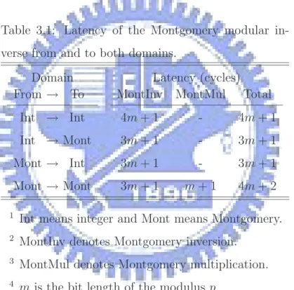
In order to convert the output to the Montgomery domain, an additional Montgomery multiplication operation is added afterward. If the input is originally in the integer do-main, i.e. A ≡ a (mod P ), then the output in the integer domain needs m iterations more than output in the Montgomery domain. The latencies of the Montgomery modular inverse from and to both domains are listed in the Table3.1:
Table 3.1: Latency of the Montgomery modular in-verse from and to both domains.
Domain Latency (cycles)
From → To Int → Int Int → Mont Mont → Int Mont → Mont
MontInv MontMul Total
4m + 1 - 4m + 1
3m + 1 - 3m + 1
3m + 1 - 3m + 1
3m + 1 m + 1 4m + 2
1 Int means integer and Mont means Montgomery. 2 MontInv denotes Montgomery inversion.
3 MontMul denotes Montgomery multiplication. 4 m is the bit length of the modulus p.
3.3
Modular Division
3.3.1
Multiplication after Inversion
The modular division operation is traditionally accomplished by modular inversion followed by modular multiplication since the modular division is believed to be slow. It
can be applied to the computation of the parameter λ in ECC. Given two integers a and b in integer domain, divide a by b is done as follows:
c ≡ a
b (mod p) (3.30)
≡ a · b−1 (mod p) (3.31)
which can be performed by modular inverse followed by modular multiplication. But in ECC, operands are represented in the Montgomery domain. Given two integers A and B in the Montgomery domain, the Montgomery modular division is defined as follows:
C ≡ MontMul(A, MontMul(MontInv(B), r2)) (3.32)
≡ a · b−1· r (mod p) (3.33)
≡ c · r (mod p) (3.34)
≡ MontDiv(A, B) (3.35)
One extra Montgomery multiplication is required to keep the result in the Montgomery domain. Table 3.2 shows the latency of traditional method using a Montgomery inversion followed by a Montgomery multiplication.
Table 3.2: Latency of modular division using traditional method from and to both domain
Domain Latency (cycles)
From → To Int → Int Int → Mont Mont → Int Mont → Mont
MonInv MonMul MonMul Total
3m + 1 m + 1 - 4m + 2
3m + 1 m + 1 m + 1 5m + 3
3m + 1 m + 1 - 4m + 2
3m + 1 m + 1 m + 1 5m + 3
3.3.2
Modular Division Algorithm
Given an m-bit modulus p, the modular division of two integers a, b ∈ GF (p), where b 6= 0, is defined as the integer x,