應用於三維繪圖系統之可重組式深度緩衝區壓縮演算法設計與實作

全文

(1)國立交通大學資訊科學與工程研究所碩士論文. 應用於三維繪圖系統之可重組式深度緩衝區壓縮演算法設計與實作 Reconfigurable Depth Buffer Compression Design and Implementation for 3D Graphics System. 研究生：鍾宗融指導教授：范倫達. 博士. 中華民國九十七年九月.

(2) 應用於三維繪圖系統之可重組式深度緩衝區壓縮演算法設計與實作 Reconfigurable Depth Buffer Compression Design and Implementation for 3D Graphics System 研究生：鍾宗融. Student：Tzung-Rung Jung. 指導教授：范倫達博士. Advisor：Dr. Lan-Da Van. 國立交通大學資訊科學與工程研究所碩士論文 A Thesis Submitted to Institute of Computer Science and Engineering College of Computer Science National Chiao Tung University in partial Fulfillment of the Requirements for the Degree of Master in Computer Science September 2008 Hsinchu, Taiwan, Republic of China. 中華民國九十七年九月.

(3) 摘要. 應用於三維繪圖系統之可重組式深度緩衝區壓縮演算法設計與實作. 學生：鍾宗融. 指導教授：范倫達博士. 國立交通大學資訊科學與工程研究所. 摘. 要. 在本論文中，我們針對三維繪圖處理器中的深度緩衝區提出具減少頻寬需求與可重組式的壓縮演算法；根據不同的場景，從十一種壓縮模式中選擇出最適合的壓縮模式，而這十一種模式是由 2-bit DDPCM、1-bit HA、7-bit DDPCM 三種壓縮演算法所組合而成。此外，我們所提出的演算法亦支援單平面與雙平面兩種型態方塊，並能支援四種差值組合方式。在 8x8 大小方塊而且深度值長度為 16-bit 的 Teapot 場景模擬環境下，我們提出的演算法其平均壓縮比可達 1.75，而且相較於 HA 與 DDPCM 壓縮方法能夠分別改善 13.6%與 31.6%；在 8x8 大小方塊而且深度值長度為 16-bit 的 Stereoscopic polygons 場景模擬環境下，我們提出的演算法其平均壓縮比可達 1.74，而且相較於 HA 與 DDPCM 壓縮方法能夠分別改善 21.7% 與 38.1%。深度緩衝區壓縮演算法其架構具可重組式與可調式功耗之特色，使用的製程為 TSMC 0.18-um CMOS process，其晶片所佔面積為 1.13 mm2；在操作頻率為 100 MHz 與操作電壓為 1.8 伏特的情況下，未壓縮模式的最大功率消耗為 38.63 mW，單平面模式下的最大功率消耗為 22.75 mW，雙平面模式中(僅包含 rising, vertical, and horizontal cases)的最大功率消耗分別為 51.76/56.25/71.9 mW，雙平面模式中(僅 I.

(4) 摘要. 包含 falling cases)的最大功率消耗為 57.63 mW。. II.

(5) Abstract. Reconfigurable Depth Buffer Compression Design and Implementation for 3D Graphics System. Student：Tzung-Rung Jung. Advisor：Dr. Lan-Da Van. Institute of Computer Science and Engineering College of Computer Science National Chiao Tung University. ABSTRACT A less-bandwidth-required reconfigurable depth buffer compression algorithm and the corresponding power-efficient architecture have been developed for 3D graphics system. The proposed algorithm is able to adaptively compress the depth buffer data according to different-scene changes by employing 11 compression modes generated from three compression algorithms including Differential Differential Pulse Code Modulation (2-bit DDPCM), Hasselgren and Akenine-Möller’s (1-bit HA), and 7-bit DDPCM schemes. Furthermore, this reconfigurable algorithm supports one-plane and two-plane type and four kinds of combination cases. For 8x8 tile size with 16-bit depth values under the teapot benchmark, the proposed reconfigurable algorithm can achieve CR of 1.75 on average and improve 13.6% and 31.6% compared with the HA and DDPCM compression methods, respectively. For 8x8 tile size with 16-bit depth values under the Stereoscopic polygons benchmark, the proposed reconfigurable algorithm can achieve CR of 1.74 on average and improve 21.7% and 38.1% compared with the HA and DDPCM compression methods, respectively.. III.

(6) Abstract. The proposed reconfigurable power-efficient depth buffer compression architecture has been verified and implemented in TSMC 0.18-um CMOS process. The core area is of 1.13 mm2. The maximum power consumption of 38.63 mW in uncompression mode, 22.75 mW in one-plane type, 51.76/56.25/71.9 mW in two-plane type, including rising, vertical, and horizontal cases, and 57.63 mW in two-plane type, including falling cases, can be achieved at 100 MHz and with the supply voltage of 1.8V.. IV.

(7) Contents. Contents 摘. 要 .................................................................................................................... I. ABSTRACT ........................................................................................................... III CONTENTS ............................................................................................................ V LIST OF TABLES ............................................................................................... VII LIST OF FIGURES ........................................................................................... VIII Chapter 1. Introduction ......................................................................................... 1. 1.1 Motivation ..................................................................................................... 2 1.2 Thesis Organization....................................................................................... 2 Chapter 2. 3D Graphics Rendering Pipeline and Depth Buffer Compression Schemes .............................................................................................. 3. 2.1 3D Graphics Rendering Pipeline................................................................... 3 2.1.1 Geometry Subsystem ........................................................................... 4 2.1.2 Raster Subsystem ................................................................................. 4 2.1.3 Depth Buffer......................................................................................... 5 2.2 Exsisting Depth Buffer Compression Schemes ............................................ 6 2.2.1 Fast Z-Clears ........................................................................................ 6 2.2.2 Differential Differntial Pulse Code Modulation................................... 7 V.

(8) List of Tables. 2.2.3 Anchor Encoding.................................................................................. 8 2.2.4 HA Compression Scheme .................................................................... 9 2.2.5 Plane Encoding....................................................................................11 2.2.6 Depth Offset Compression ................................................................. 12 Chapter 3. Proposed Reconfigurable Compression Algorithm and Architecture ........................................................................................................... 14. 3.1 Proposed Reconfiguable Algorithm ............................................................ 14 3.1.1 Plane Type and Combination Case..................................................... 14 3.1.2 Compression Schemes ....................................................................... 16 3.1.3 Data Flow ........................................................................................... 19 3.1.4 Control-Code ...................................................................................... 25 3.1.5 Decompression ................................................................................... 25 3.2 Proposed Reconfigurable Achitecture ......................................................... 27 3.2.1 First Stage........................................................................................... 27 3.2.2 Second Stage ...................................................................................... 31 3.2.3 Third Stage ......................................................................................... 33 Chapter 4. Simulation Results and Chip Implementation ................................. 38. 4.1 Simulation Results ...................................................................................... 38 4.2 Chip Implementation ................................................................................... 42 Chapter 5. Conclusion and Future Work ........................................................... 45. Bibliography .......................................................................................................... 47. VI.

(9) List of Tables. List of Tables Chapter 3 3.1: Proposed compression modes .......................................................................... 18 3.2: Analysis of redundant computation cycles with different number of differential computation blocks. ...................................................................................... 30 3.3: Summary of number of clock cycles needed for each compression/uncompression mode. .............................................................. 37 Chapter 4 4.1: Bit width of compressed/uncompressed tile in proposed algorithm. ............... 39 4.2: Average compression ratio with 8x8 tile size................................................... 42 4.3: Chip characteristics of the proposed architecture. ........................................... 43. VII.

(10) List of Figures. List of Figures Chapter 2 2.1: 3D graphics rendering pipeline. ......................................................................... 3 2.2: Illustration of DDPCM scheme. ........................................................................ 8 2.3: Illustration of anchor encoding. ......................................................................... 9 2.4: Illustration of one-plane type compression. ..................................................... 10 2.5: Example of one-plane mode using HA compression scheme. ......................... 10 2.6: Example of two-plane mode using HA compression scheme. ..........................11 2.7: Two kinds of combination cases supported by HA compression scheme and corresponding break-point maps. ...................................................................11 2.8: Example of plane encoding. ............................................................................. 12 2.9: Illustration of depth offset compression........................................................... 13 Chapter 3 3.1: Two-plane type of the proposed reconfigurable algorithm. ............................. 15 3.2: Four kinds of combination cases supported by the proposed algorithm and corresponding break-point maps. .................................................................. 16 3.3: (a) Data flow illustration of the proposed reconfigurable depth buffer compression in one-plane type. ..................................................................... 20 VIII.

(11) List of Figures. 3.3: (b) Data flow illustration of the proposed reconfigurable depth buffer compression in two-plane type for rising/vertical/horizontal cases. ............. 20 3.3: (c) Data flow illustration of the proposed reconfigurable depth buffer compression in two-plane type for falling cases. .......................................... 21 3.3: (d) Data flow illustration of the proposed reconfigurable depth buffer compression in uncompression mode for case 1. .......................................... 21 3.3: (e) Data flow illustration of the proposed reconfigurable depth buffer compression in uncompression mode for case 2. .......................................... 22 3.3: (f) Data flow illustration of the proposed reconfigurable depth buffer compression in uncompression mode for case 3. .......................................... 22 3.4: Example of uncompressio mode for case 2. .................................................... 23 3.5: Control-code and break point. .......................................................................... 25 3.6: Data flow illustration of decompression. ......................................................... 26 3.7: Block diagram of the reconfigurable compression architecture. ..................... 29 3.8: Block diagram of folded differential computation ........................................... 30 3.9: Block diagram of data reorder architecture...................................................... 31 3.10: Block diagram of break-point map generation .............................................. 31 3.11: Block diagram of break-point check for determining uncompression mode. 32 3.12: Block diagram of break-point check. ............................................................. 32 3.13: Block diagram of two-plane differential combination. .................................. 34 3.14: Block diagram of the compression scheme selection. ................................... 34 3.15: Packing format. .............................................................................................. 35 IX.

(12) List of Figures. Chapter 4 4.1: (a) Teapot and (b) stereoscopic polygons......................................................... 40 4.2: Proposed algorithm vs. the 1-bit HA compression scheme for teapot scenario. ....................................................................................................................... 40 4.3: Proposed algorithm vs. the 2-bit DDPCM compression scheme for teapot scenario. ........................................................................................................ 41 4.4: Proposed algorithm vs. the 1-bit HA compression scheme for stereoscopic polygons scenario. ......................................................................................... 41 4.5: Proposed algorithm vs. the 2-bit DDPCM compression scheme for stereoscopic polygons scenario. .................................................................... 42 4.6: Chip layout of the proposed architecture. ........................................................ 44. X.

(13) Chapter 1. Chapter. Introduction. 1. Introduction Recently, the 3D computer graphics are widely used in many applications such as mobile phones, GPS (Global Positioning System), digital TV [1] , games, biomedical applications [2] , where these applications usually use complex GUI (graphical user interface) to generate better 3D images. There have been much research and development on the 3D graphics algorithms and systems for mobile devices [3] [4] [5] [6] [7] [8] [9] [10] [11] . It is manifest that 3D computer graphics system requires extremely high memory bandwidth to process. On the other hand, with the growth of complexity of 3D scenes, the amount of data computation increases substantially. Therefore, in the bandwidth-limited system, how to efficiently compress the depth buffer data to save bandwidth becomes a significant research issue. Fast z-clears compression algorithm [15] uses a dedicated flag to indicate whether a tile is cleared. The DDPCM scheme [16] , Anchor encoding [17] , HA compression scheme [21] are effective compression algorithms to exploit the continuity of interpolated depth values. The plane encoding scheme presented in [19] applies the concept of indexing to compress tiles. The depth offset compression [20] saves the differentials based on the Z-max value (maximum depth value) and Z-min value (minimum depth value) in a tile. Morein [22] presented an overview of Z-buffer architecture for reducing memory bandwidth and number of pixels drawn. Chen and Lee [23] proposed two-level hierarchical Z-buffer for saving memory bandwidth and 1.

(14) Chapter 1. Introduction. compression management. Yu and Kim [24] addressed an algorithm of depth filter for early depth test in a 3D rendering engine by adding extra hardware in the front of the per-pixel pipeline in a rasterizer and an adaptive block into the conventional depth test block.. 1.1 Motivation Since the compression performance of these existing algorithms is limited and they cannot adaptively compress according to different 3D scenes, we are motivated to propose a reconfigurable depth buffer compression algorithm. On the other hand, how to design the power-efficient depth buffer compression architecture is also an important issue.. 1.2 Thesis Organization The rest of the thesis is organized as follows. A brief review of 3D graphics rendering pipeline and existing depth buffer compression algorithms are described in Chapter 2. In Chapter 3, the proposed reconfigurable algorithm and architecture have been presented. The simulation results and chip implementation are addressed in Chapter 4. Last, brief statements conclude the presentation of this thesis.. 2.

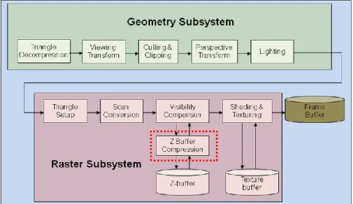
(15) Chapter 2. 3D Graphics Rendering pipeline and Depth Buffer Compression Schemes. Chapter. 2. 3D Graphics Rendering Pipeline and Depth Buffer Compression Schemes In this chapter, we will introduce the fundamental 3D graphics pipeline and existing depth buffer compression algorithms. 2.1 3D Graphics Rendering Pipeline In this section, a brief overview of 3D graphics rendering pipeline is introduced. Fig. 2.1 shows the conventional rendering pipeline. Polygon-based rendering is one of the mainstream methods to generate 3D graphics [19] . Generally, the pipeline can be divided into two subsystems including the geometry subsystem and raster subsystem.. Fig. 2.1. 3D graphics rendering pipeline. 3.

(16) Chapter 2. 3D Graphics Rendering pipeline and Depth Buffer Compression Schemes. 2.1.1 Geometry Subsystem Generally, the geometry subsystem can be subdivided into five stages, including triangle decompression, viewing transform, culling and clipping, perspective transform, and lighting. Before viewing transform, the geometry subsystem receives a triangle mesh composed of triangles. After triangle decompression, the geometry subsystem transforms 3D objects from the world space to the viewing space, that is called viewing transformation. Because some triangles are of invisible triangles, such as back-faced triangles and too small triangles, or outside of the viewing volume, they can be culled and clipped as soon as possible for reducing the unnecessary data computation. This stage is referred to as culling and clipping. Perspective transformation will transform 3D objects from the viewing space to the projection space, i.e. 3D coordinate of an object will be mapped into 2D coordinate. The lighting operation in the geometry subsystem performs lighting equations on vertices. Generally, these equations are complex for simulating lighting effect in the real world.. 2.1.2 Raster Subsystem The raster subsystem renders the transformed polygons generated from the geometry subsystem to the monitor pixel-by-pixel. The first stage of the raster subsystem is triangle setup for preparing data about triangular shape, bounding rectangle, texture coordinates, color, and etc. After triangle setup, the raster subsystem will interpolate all attributes of each pixel inside a triangle. These operations are called scan conversion. Visibility comparison in the raster subsystem is used to detect whether a pixel is covered by other pixels. If the pixel A is covered by the pixel B, the pixel A will be dropped immediately for eliminating unnecessary operations. The Z-buffer saves the depth values corresponding to the pixels not covered by other pixels at that time. 4.

(17) Chapter 2. 3D Graphics Rendering pipeline and Depth Buffer Compression Schemes. The final stage of the raster subsystem is shading and texturing. At this stage, besides the flat shading and Gouraud shading, some advanced and complex lighting algorithms, such as Phong shading, may be applied to every pixel. Lighting is used to calculate the colors of vertices or pixel related to the lighting source in the 3D space. Therefore, the lighting model is used to describe the relationship between vertices or pixels and the lighting source. One of the popular lighting models is Phong model expressed in the following equation.. I  kaIa  kdId( N  L)  ksIs( N  H ) ns. (2.1). where Ia denotes the intensity of the ambient light, Is, L, N denote the intensity of the light source, the unit vector from pixel to the light source, and the normal vector of the pixel, respectively. H equals (L+V)/2, V denotes the vector from the pixel to the view, ns describes the gloss to model the highlight, and ka,kd, and ks are the coefficients to model the characteristic of the material. Texture mapping needs to access texture buffer with huge memory bandwidth and apply mapping equations. However, texture mapping provides an effective way to mimic the realistic of real world on the display. Some algorithms and architectures are presented about the texture filter [12] and texture compression [13] [14] . The output of the raster subsystem will be transferred to the frame buffer for displaying on the monitor.. 2.1.3 Depth Buffer In this section, the depth buffer is introduced. The depth buffer, i.e. Z buffer, saves the depth values corresponding to the pixels at that time. In order to determine whether a pixel is covered by other pixels, the depth test will be performed. The depth test reads and writes the depth buffer many times whenever a pixel has to be tested. 5.

(18) Chapter 2. 3D Graphics Rendering pipeline and Depth Buffer Compression Schemes. Thus, the depth test results in the heavy bandwidth traffic on memory bus. To reduce the heavy memory accesses, more efficient compression will be highly demanded. In this thesis, a 4x4 or 8x8 pixels called a tile will be access from the depth buffer. There are some schemes depending on the depth buffer for reducing memory access, such as hierarchical Z buffer [27] , Z-max culling, Z-min culling [26] , and depth filter [28] [29] . Besides the filter-based memory-accessing reduction techniques, the offset-based data compression schemes are investigated to reduce memory bus traffic. The next section will briefly introduce this kind of techniques.. 2.2 Existing Depth Buffer Compression Schemes In this section, we give an overview of the state-of-the-art compression schemes. Generally, these schemes can be divided into three categories, fast z-clears, differential differential pulse code modulation (DDPCM), anchor encoding, HA compression scheme, plane encoding, and depth offset compression scheme. The descriptions are as follows.. 2.2.1 Fast Z-Clears Fast z-clears [15] is a simple compression algorithm and easy to be implemented. A dedicated bit is used to indicate whether the tile is cleared. If the tile is cleared, we can only write back the latest depth values to depth buffer without reading the depth buffer to update the depth values.. 6.

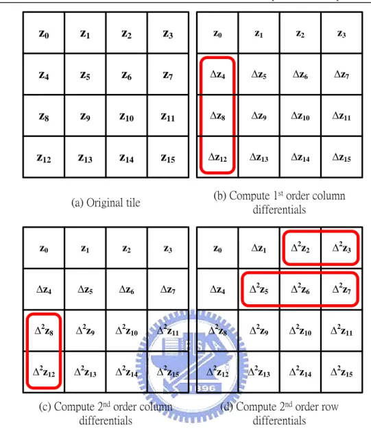
(19) Chapter 2. 3D Graphics Rendering pipeline and Depth Buffer Compression Schemes. 2.2.2 Differential Differential Pulse Code Modulation The Differential Differential Pulse Code Modulation (DDPCM) [16] scheme is widely applied to the data compression since the depth values are obtained by linearly interpolation in the screen space. DeRoo et al. [16]. proposed a depth buffer. compression algorithm as illustrated in Fig. 2.2., where the notations are defined in the following equations describe the notations in Fig. 2.2. △z4 = z4 – z0. (2.2a). △z8 = z8 – z4. (2.2b). △z12 = z12 – z8. (2.2c). △z28 = △z8 – △z4. (2.2d). △z212 = △z12 –△z8. (2.2e). △z22 = z2 – z1 – △z1. (2.2f). △z23 = z3 – z2 – △z2. (2.2g). △z25 = △z5 – △z4. (2.2h). △z26 = △z6 – △z5. (2.2i). △z27 = △z7 – △z6. (2.2j). The DDPCM scheme can achieve the high compression ratio (CR) on 8x8 tile size, where CR is defined as follows.. CR . uncompressed bits compressed bits. (2.3). DeRoo et al. also proposed an extended depth buffer compression scheme, called two-plane mode, in order to handle specific cases that tile can be separated into two planes.. 7.

(20) Chapter 2. 3D Graphics Rendering pipeline and Depth Buffer Compression Schemes. z0. z1. z2. z3. z0. z1. z2. z3. z4. z5. z6. z7. ∆z4. ∆z5. ∆z6. ∆z7. z8. z9. z10. z11. ∆z8. ∆z9. ∆z10. ∆z11. z12. z13. z14. z15. ∆z12. ∆z13. ∆z14. ∆z15. (b) Compute 1st order column differentials. (a) Original tile. z0. z1. z2. z3. z0. ∆z1. ∆2z2. ∆2z3. ∆z4. ∆z5. ∆z6. ∆z7. ∆z4. ∆2z5. ∆2z6. ∆2z7. ∆2z8. ∆2z9. ∆2z10. ∆2z11. ∆2z8. ∆2z9. ∆2z10. ∆2z11. ∆2z12. ∆2z13. ∆2z14. ∆2z15. ∆2z12. ∆2z13. ∆2z14. ∆2z15. (c) Compute 2nd order column differentials. (d) Compute 2nd order row differentials. Fig. 2.2. Illustration of DDPCM scheme.. 2.2.3 Anchor Encoding Van Dyke and Margeson [17] proposed a compression scheme similar to the DDPCM scheme. Instead of setting upper left pixel as a reference point, this compression algorithm selects a fixed anchor point, z0, from other positions in a tile as shown in the Fig. 2.3. All we have to save are 16-bit anchor point, 7-bit x differential, 7-bit y differential and 5-bit 2nd order differentials. In fact, we cannot obtain better compression ratio by anchor encoding than that of the DDPCM scheme [21] . 8.

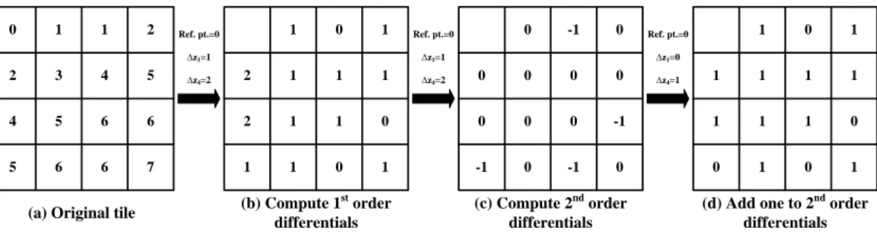
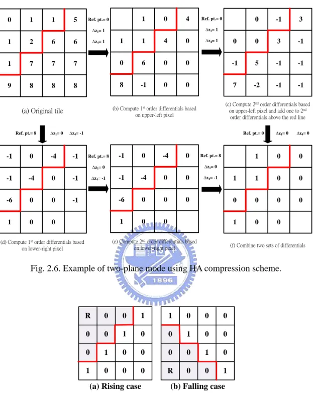
(21) Chapter 2. 3D Graphics Rendering pipeline and Depth Buffer Compression Schemes. p. p. p. p. p. z0. ∆x. p. p. ∆y. p. p. p. p. p. p. Fig. 2.3. Illustration of anchor encoding.. 2.2.4 HA Compression Scheme Hasselgren and Akenine-Möller proposed a state-of-the-art depth buffer compression scheme, which can achieve high CR by exploiting the continuity of interpolated depth values in the screen space [21] . The plane mode means how many reference points will be used to compute differentials. In HA compression scheme, one-plane and two-plane modes are included. In one-plane mode, only one reference point is used to achieve compression; in two-plane mode, two reference points are used. The operations of the one-plane mode are illustrated in the Fig. 2.4. The two 1st order differentials are △z1 and △z4. Except z0, △z1 ,and △z4, the remaining values are called 2nd order differentials. The example of the one-plane mode is illustrated in Fig. 2.5. From the one-plane mode example, the 2nd order differentials are saved in only 1 bit that is the reason why this algorithm can achieve better CR than other compression schemes. In two-plane mode, two one-plane-mode operations will be applied according to two different reference points. Fig. 2.6 depicts an example of two-plane mode. Furthermore, there are two kinds of combination cases, as shown in Fig. 2.7, including rising and falling cases in the two-plane mode, where R means the reference point. In the rising case, the slope of 9.

(22) Chapter 2. 3D Graphics Rendering pipeline and Depth Buffer Compression Schemes. break points is rising. That is why this condition called rising case. Similarly, the slope of falling case is falling. These two kinds of combination cases can increase the compression flexibility to achieve higher compression ratio. The two-plane mode has break-point information which is composed of 0’s and 1’s. Because we have to combine two sets of differentials with two different reference points, break points indicate which differential set should be chosen for combination. The positions of break points indicate that the value of the 2nd order differentials is larger than that of HA compression scheme. Additionally, this scheme as shown in the Fig. 2.6 can handle two-plane mode cases rather than a fixed-position-reference-point scheme of the extended DDPCM scheme. z0. z1. z2. z3. z0. ∆z1. ∆2z2. ∆2z3. z4. z5. z6. z7. ∆z4. ∆2z5. ∆2z6. ∆2z7. z8. z9. z10. z11. ∆2z8. ∆2z9. ∆2z10. ∆2z11. z12. z13. z14. z15. ∆2z12. ∆2z13. ∆2z14. ∆2z15. Δz i  zi  z0 , i  1, 4 zi  z(i  4)  Δz 4 , i  8,12  Δ 2 zi    zi  z(i  1)  Δz1, i  2, 3, 5, 6, 7, 9, 10, 11, 13, 14, 15. Fig. 2.4. Illustration of one-plane mode compression.. 0. 1. 1. 2. 1. 0. 1. 2. 3. 4. 5. 2. 1. 1. 1. 4. 5. 6. 6. 2. 1. 1. 5. 6. 6. 7. 1. 1. 0. Ref. pt.=0. 0. -1. 0. 0. 0. 0. 0. 0. 0. 0. 0. 1. -1. 0. -1. ∆z1=1 ∆z4=2. Ref. pt.=0. 0. 1. 1. 1. 1. 1. -1. 1. 1. 1. 0. 0. 0. 1. 0. ∆z1=1 ∆z4=2. st. (a) Original tile. 1. ∆z1=0. nd. (b) Compute 1 order differentials. Ref. pt.=0. (c) Compute 2 order differentials. ∆z4=1. (d) Add one to 2 order differentials. Fig. 2.5. Example of one-plane mode using HA compression scheme.. 10. 1 nd.

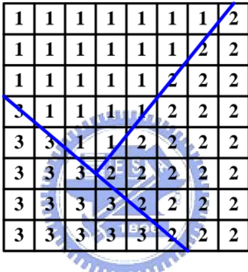
(23) Chapter 2. 0. 1. 1. 5. 1. Ref. pt.= 0. 0. 3D Graphics Rendering pipeline and Depth Buffer Compression Schemes. 4. 0. 3. -1. 0. 7. 0. 6. 0. 0. -1. 5. -1. -1. 8. 8. -1. 0. 0. 7. -2. -1. -1. 6. 1. 7. 7. 9. 8. 8. ∆z4= 1. (c) Compute 2nd order differentials based on upper-left pixel and add one to 2nd order differentials above the red line. (b) Compute 1st order differentials based on upper-left pixel. (a) Original tile. -4. 0. 4. 6. 0. ∆z4= 1. 1. 2. -1. 3. 1. 1. ∆z1= 0. -1. ∆z1= 1. ∆z1= 1. Ref. pt.= 8. 0. Ref. pt.= 0. ∆z4= -1. -1. Ref. pt.= 0. Ref. pt.= 8. -1. 0. -4. 0. -4. 0. -1. -6. 0. 0. -1. 1. 0. 0. ∆z4= -1. 1. 0. 0. 1. 1. 0. 0. 0. 0. 0. 0. 1. 0. 0. Ref. pt.= 8. -1. -4. 0. 0. -6. 0. 0. 0. 1. 0. 0. ∆z4= -1. (e) Compute 2nd order differentials based on lower-right pixel. (d) Compute 1st order differentials based on lower-right pixel. ∆z4= 0. ∆z1= 0. ∆z1= 0. -1. ∆z1= 0. (f) Combine two sets of differentials. Fig. 2.6. Example of two-plane mode using HA compression scheme.. R. 0. 0. 1. 1. 0. 0. 0. 0. 0. 1. 0. 0. 1. 0. 0. 0. 1. 0. 0. 0. 0. 1. 0. 1. 0. 0. 0. R. 0. 0. 1. (a) Rising case. (b) Falling case. Fig. 2.7. Two kinds of cases supported by HA compression scheme and corresponding break-point maps.. 2.2.5 Plane Encoding Different from the compression algorithms with the use of the continuity of interpolated depth values in the screen space, plane encoding labels triangles in a range 11.

(24) Chapter 2. 3D Graphics Rendering pipeline and Depth Buffer Compression Schemes. of tiles and saves these index numbers eventually. When a pixel is rendered, the depth value corresponding to the coordinate has to be computed. Van Hook [18] and Liang et al. [19] both presented compression schemes similar to the plane encoding. Fig. 2.8 shows the abstract concept of the plane encoding. The plane encoding can handle several overlapping triangles in a single tile, which is suitable for large tile size. The drawback is that it must store indices and the corresponding counter value in depth tile cache [21] .. 1. 1. 1. 1. 1. 1. 1. 2. 1. 1. 1. 1. 1. 1. 2. 2. 1. 1. 1. 1. 1. 2. 2. 2. 3. 1. 1. 1. 1. 2. 2. 2. 3. 3. 1. 1. 2. 2. 2. 2. 3. 3. 3. 2. 2. 2. 2. 2. 3. 3. 3. 3. 2. 2. 2. 2. 3. 3. 3. 3. 3. 2. 2. 2. Fig. 2.8. Example of plane encoding.. 2.2.6 Depth Offset Compression Morein and Natale [20] presented depth offset compression as illustrated in Fig. 2.9. For tile-based rendering, assume that we save the Z-max (maximum depth value) value and Z-min value (minimum depth value) of a tile. The depth values of a tile will be categorized into to the representable and unrepresentable ranges. The representable ranges consist of two regions based on Z-max value and Z-min value. Hasselgren and Akenine-Möller [21] also have presented a modified scheme consisting of two kinds of representable ranges in depth offset compression, one with 12. 12.

(25) Chapter 2. 3D Graphics Rendering pipeline and Depth Buffer Compression Schemes. bits per pixel used to store the offsets, and one with 16 bits per pixel. If the minimum and maximum values are already stored in the tile table, this scheme uses 12 or 16 bits per pixel, and results in a higher CR [25] . If we stored the Z-max and Z-min values of the compressed tile, this scheme can be applied without extra cost. It cannot work well for high CR value, but obtains excellent compression probabilities for low CR value [21] . Z-max value. Z-min value. Representable Range. Unrepresentable Range. Representable Range. Fig. 2.9. Illustration of depth offset compression.. 13.

(26) Chapter 3. Proposed Reconfigurable Compression Algorithm and Architecture. Chapter. 3. Proposed Reconfigurable Compression Algorithm and Architecture In this chapter, we propose a reconfigurable algorithm and architecture for depth buffer compression. According to the different scene changes, the proposed algorithm is capable of adaptively employing three compression schemes including the 2-bit DDPCM [16] , 1-bit HA [21] , and 7-bit DDPCM schemes to generate 11 compression modes. The presented 7-bit DDPCM scheme similar to the 2-bit DDPCM scheme makes use of 7 bits to save each 2nd order differential. The data flow graph of the proposed algorithm demonstrates the difference among different mode compressions. The corresponding reconfigurable architecture consisting of three stages will be issued at the end of this chapter.. 3.1 Proposed Reconfigurable Algorithm In this session, the proposed algorithm will be discussed in detail by data flow graph.. 3.1.1 Plane Type and Combination Case In the proposed algorithm, the plane type also referred as to the plane mode in the 1-bit HA compression scheme is also concerned. Different from the HA scheme [21] , 14.

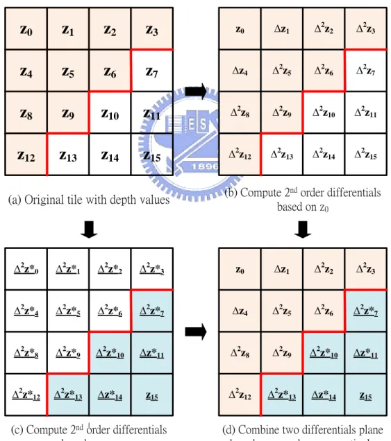
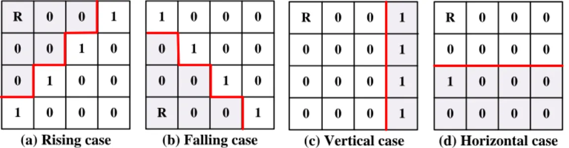
(27) Chapter 3. Proposed Reconfigurable Compression Algorithm and Architecture. in the proposed algorithm, the compression scheme selection (CSS), which will be discussed later, in the proposed algorithm is performed after two-plane differential combination for hardware-oriented design. Fig. 3.1 illustrates how to compute two sets of differentials according to two different reference points and how to combine the two planes. Furthermore, we extend original two combination cases into four combination cases, as shown in Fig. 3.2, including rising, falling, vertical and horizontal cases in the two-plane type. These four kinds of combination cases can increase the compression flexibility to achieve higher compression ratio.. z0. z1. z2. z3. z0. ∆z1. ∆2z2. ∆2z3. z4. z5. z6. z7. ∆z4. ∆2z5. ∆2z6. ∆2z7. z8. z9. z10. z11. ∆2z8. ∆2z9. ∆2z10. ∆2z11. z12. z13. z14. z15. ∆2z12. ∆2z13. ∆2z14. ∆2z15. (b) Compute 2nd order differentials based on z0. (a) Original tile with depth values. ∆2z*0. ∆2z*1. ∆2z*2. ∆2z*3. z0. ∆z1. ∆2z2. ∆2z3. ∆2z*4. ∆2z*5. ∆2z*6. ∆2z*7. ∆z4. ∆2z5. ∆2z6. ∆2z*7. ∆2z*8. ∆2z*9. ∆2z*10. ∆z*11. ∆2z8. ∆2z9. ∆2z*10. ∆z*11. ∆2z*12. ∆2z*13. ∆z*14. z15. ∆2z12. ∆2z*13. ∆z*14. z15. (c) Compute 2nd order differentials based on z15. (d) Combine two differentials plane based on z0 and z15, respectively. Fig. 3.1. Two-plane type of the proposed reconfigurable algorithm.. 15.

(28) Chapter 3. Proposed Reconfigurable Compression Algorithm and Architecture. R. 0. 0. 1. 1. 0. 0. 0. R. 0. 0. 1. R. 0. 0. 0. 0. 0. 1. 0. 0. 1. 0. 0. 0. 0. 0. 1. 0. 0. 0. 0. 0. 1. 0. 0. 0. 0. 1. 0. 0. 0. 0. 1. 1. 0. 0. 0. 1. 0. 0. 0. R. 0. 0. 1. 0. 0. 0. 1. 0. 0. 0. 0. (a) Rising case. (b) Falling case. (c) Vertical case. (d) Horizontal case. Fig. 3.2. Four kinds of combination cases supported by the proposed algorithm and corresponding break-point maps.. 3.1.2 Compression Schemes So as to increase the higher CR of the depth buffer compression, we employ three kinds of compression schemes in the proposed algorithm. These schemes including 1-bit HA [21] , 2-bit DDPCM [16] , and 7-bit DDPCM schemes can be adaptively chosen with the aim of the highest compression ratio. The difference among these three algorithms is the bit length for storing each value of differential. Through the 1-bit HA and 2-bit DDPCM schemes, we can use only one bit and two bits to store each differential, respectively. Although the 1-bit HA and 2-bit DDPCM schemes are useful to save differentials, these two compression schemes still limit CR for more complex 3D scenes. Concerning more stable CR, we decide to use 7-bit DDPCM in this thesis. The following attributes summarize the conditions for each compression scheme. The ranges of each compression scheme can be addressed as follows. The 1-bit HA scheme covers the differential set of {0,1} and 2-bit DDPCM scheme covers the differential set of {1,0,1} , and the differential set of the 7-bit DDPCM scheme covers the differential set of {-64,-63, ,61,62,63} . Additionally, the HA scheme can be divided into two types. The type 1 HA scheme means all the 2nd order differentials are the elements of the set {-1,0}. These 2nd order differentials will be added by one and the 1st order differentials will be subtracted by one such that all the differentials are the 16.

(29) Chapter 3. Proposed Reconfigurable Compression Algorithm and Architecture. elements of the set of {1,0}. Therefore, each differential can be saved in only one bit. On the other hand, the type 2 HA scheme means all the differentials are already the elements of the set of {1,0} without addition and subtraction. All compression schemes can be applied to one-plane and two-plane types. In addition, we divide a tile into two parts including vertical and horizontal parts. The horizontal part stands for the positions, z2, z3, z5, z6, z7, z9, z10, z11, z13, z14, and z15, in Fig. 2.4. The vertical part stands for the positions, z8 and z12, in Fig. 2.4. In these two parts, different compression schemes can be applied. For example, the vertical part applies the 1-bit HA scheme and the horizontal part applies the 2-bit DDPCM scheme. According to the combination of plane type and schemes used, the 11 compression modes can be obtained in Table 3.1. Consequently, owing to two-plane types by five schemes (i.e., ten modes are generated) and one uncompression mode, the number of modes is 11.. 17.

(30) Chapter 3. Proposed Reconfigurable Compression Algorithm and Architecture. Table 3.1. Proposed compression modes. Compression Mode. Mode Description. Name OP-HA-HA. 1-bit HA scheme applied in both of the vertical and horizontal parts under one-plane type. OP-2bDDPCM-HA. 2-bit DDPCM and 1-bit HA schemes are applied in vertical and horizontal parts, respectively, under one-plane type. OP-7bDDPCM-HA. 7-bit DDPCM and 1-bit HA schemes are applied in the vertical and horizontal parts, respectively, under one-plane type. OP-7bDDPCM-2bDDP. 7-bit DDPCM and 2-bit DDPCM schemes are applied in the. CM. vertical and horizontal parts, respectively, under one-plane type. OP-7bDDPCM. 7-bit DDPCM scheme is applied in both of the vertical and. -7bDDPCM. horizontal parts under one-plane type. TP-HA-HA. 1-bit HA scheme is applied in both of the vertical and horizontal parts under two-plane type. TP-2bDDPCM-HA. 2-bit DDPCM and 1-bit HA schemes are applied in the vertical and horizontal parts, respectively, under two-plane type. TP-7bDDPCM-HA. 7-bit DDPCM and 1-bit HA schemes are applied in the vertical and horizontal parts, respectively, under two-plane type. TP-7bDDPCM-2bDDP. 7-bit DDPCM and 2-bit DDPCM schemes are applied in the. CM. vertical and horizontal parts, respectively, under two-plane type. TP-7bDDPCM. 7-bit DDPCM scheme is applied in both of the vertical and. -7bDDPCM. horizontal parts under two-plane type. Uncompression. Unsupported combination cases in two-plane type. 18.

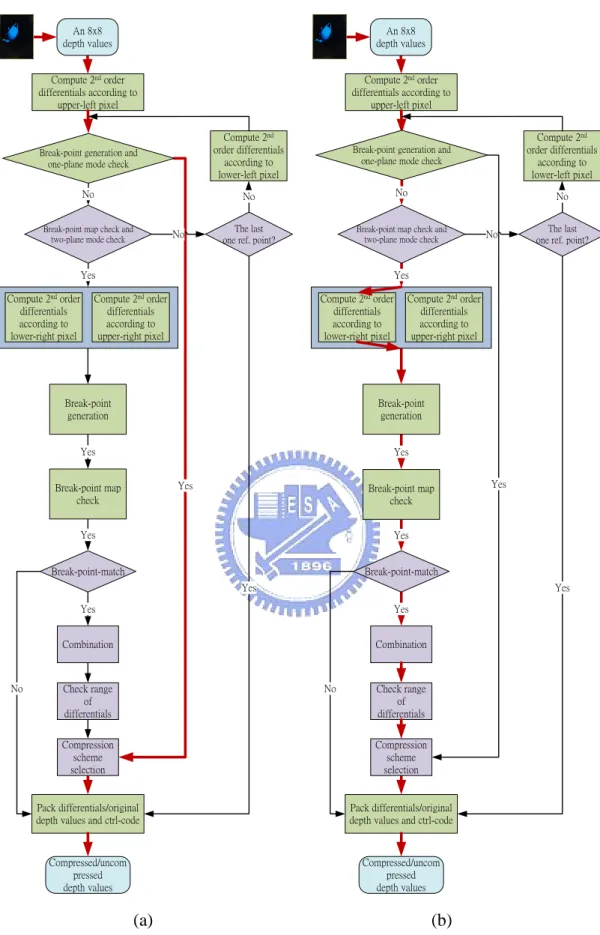
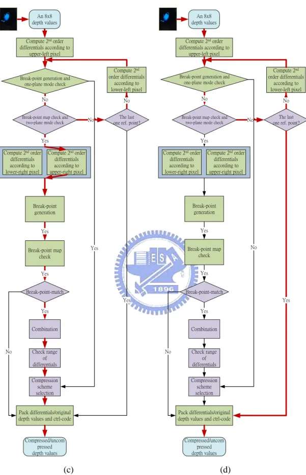
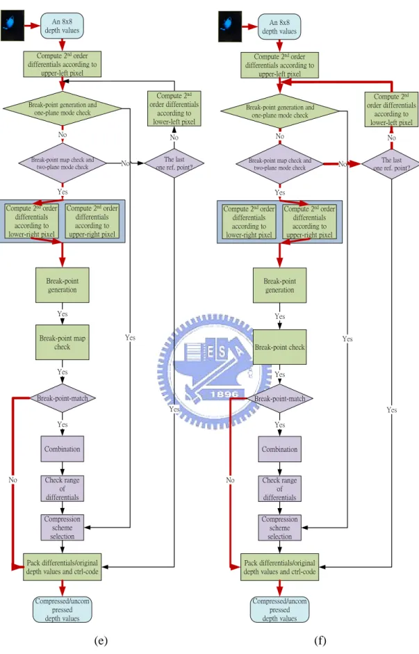
(31) Chapter 3. Proposed Reconfigurable Compression Algorithm and Architecture. 3.1.3 Data Flow The data flows of the proposed algorithm as depicted in Fig. 3.3 (a)-(f) are described in the following, where the coarse-solid lines in Fig. 3.3 (a)-(f) indicate the flows according to different cases. Fig. 3.3 (a) shows one-plane type; Fig. 3.3 (b) shows two-plane type including rising, vertical, and horizontal cases; Fig. 3.3 (c) shows two-plane type, including falling cases; Fig. 3.3 (d)-(f) show the data flow in uncompression mode. In details, Fig. 3.3 (d) illustrates the two sets of break points according to the upper-left and lower-left pixels are unsupported. Fig. 3.3 (e) and (f) show the set of differentials according to the 2nd reference point in two-plane type including rising, vertical, horizontal, and falling cases does not pass break-point-match. Fig. 3.4 shows an example of uncomoression mode for case 2. Furthermore, assume that only 2-bit DDPCM scheme is applied in Fig. 3.4. In Fig. 3.4, the break points of differentials according to the upper-left pixel are determined as a rising case. However, the break points of differentials according to the lower-right pixel are determined as an uncompressed case. Because the two sets of break points are determined as different cases, this kind of tile finally is classified into the uncompression mode.. 19.

(32) Chapter 3. Proposed Reconfigurable Compression Algorithm and Architecture. An 8x8 depth values. An 8x8 depth values. Compute 2nd order differentials according to upper-left pixel. Compute 2nd order differentials according to upper-left pixel. Break-point generation and one-plane mode check. Compute 2nd order differentials according to lower-left pixel. Break-point generation and one-plane mode check. Compute 2nd order differentials according to lower-left pixel. No. No. No. No. The last one ref. point?. Break-point map check and two-plane mode check. Break-point map check and two-plane mode check. No. Yes Compute 2nd order differentials according to lower-right pixel. No. The last one ref. point?. Yes. Compute 2nd order differentials according to upper-right pixel. Compute 2nd order differentials according to lower-right pixel. Compute 2nd order differentials according to upper-right pixel. Break-point generation. Break-point generation. Yes. Yes Yes. Break-point map check. Break-point map check. Yes. Yes. Yes. Break-point-match. Break-point-match Yes. No. Yes. Yes. Yes. Combination. Combination. No. Check range of differentials. Check range of differentials. Compression scheme selection. Compression scheme selection. Pack differentials/original depth values and ctrl-code. Pack differentials/original depth values and ctrl-code. Compressed/uncom pressed depth values. Compressed/uncom pressed depth values. (a). (b). Fig. 3.3. (a) Data flow illustration of the proposed reconfigurable depth buffer compression in one-plane type. (b) Data flow illustration of the proposed reconfigurable depth buffer compression in two-plane type for rising/vertical/horizontal cases. 20.

(33) Chapter 3. Proposed Reconfigurable Compression Algorithm and Architecture. An 8x8 depth values. An 8x8 depth values. Compute 2nd order differentials according to upper-left pixel. Compute 2nd order differentials according to upper-left pixel. Break-point generation and one-plane mode check. Compute 2nd order differentials according to lower-left pixel. Break-point generation and one-plane mode check. Compute 2nd order differentials according to lower-left pixel. No. No. No. No. The last one ref. point?. Break-point map check and two-plane mode check. Break-point map check and two-plane mode check. No. Compute 2nd order differentials according to upper-right pixel. Compute 2nd order differentials according to lower-right pixel. Compute 2nd order differentials according to upper-right pixel. Break-point generation. Break-point generation. Yes. Yes Yes. Break-point map check. Break-point map check. No. Yes. Yes Break-point-match. Break-point-match Yes. No. The last one ref. point?. Yes. Yes Compute 2nd order differentials according to lower-right pixel. No. Yes. Yes. Yes. Combination. Combination. No. Check range of differentials. Check range of differentials. Compression scheme selection. Compression scheme selection. Pack differentials/original depth values and ctrl-code. Pack differentials/original depth values and ctrl-code. Compressed/uncom pressed depth values. Compressed/uncom pressed depth values. (c). (d). Fig. 3.3. (c) Data flow illustration of the proposed reconfigurable depth buffer compression in two-plane type for falling cases. (d) Data flow illustration of the proposed reconfigurable depth buffer compression in uncompression mode for case 1. 21.

(34) Chapter 3. Proposed Reconfigurable Compression Algorithm and Architecture. An 8x8 depth values. An 8x8 depth values. Compute 2nd order differentials according to upper-left pixel. Compute 2nd order differentials according to upper-left pixel. Break-point generation and one-plane mode check. Compute 2nd order differentials according to lower-left pixel. Break-point generation and one-plane mode check. Compute 2nd order differentials according to lower-left pixel. No. No. No. No. The last one ref. point?. Break-point map check and two-plane mode check. Break-point map check and two-plane mode check. No. Yes Compute 2nd order differentials according to lower-right pixel. No. Yes. Compute 2nd order differentials according to upper-right pixel. Compute 2nd order differentials according to lower-right pixel. Compute 2nd order differentials according to upper-right pixel. Break-point generation. Break-point generation. Yes. Yes. Yes. Break-point map check. Yes Break-point check. Yes. Yes. Break-point-match. Break-point-match. Yes. No. The last one ref. point?. Yes. Yes. Yes. Combination. Combination. Check range of differentials. No. Check range of differentials. Compression scheme selection. Compression scheme selection. Pack differentials/original depth values and ctrl-code. Pack differentials/original depth values and ctrl-code. Compressed/uncom pressed depth values. Compressed/uncom pressed depth values. (e). (f). Fig. 3.3. (e) Data flow illustration of the proposed reconfigurable depth buffer compression in uncompression mode for case 2. (f) Data flow illustration of the proposed reconfigurable depth buffer compression in uncompression mode for case 3. 22.

(35) Chapter 3. 0. 1. Proposed Reconfigurable Compression Algorithm and Architecture. 2. 3. Ref. pt.= 0. 0. 0. 0. 0. 0. -1. 0. 0. ∆z1= 1 ∆z4= 5. 5. 5. 6. 7. 9. 11. 13. 16. -1. 1. 1. 2. 13. 13. 16. 16. -1. -1. 2. -1. (b) Compute 2nd order differentials based on upper-left pixel. (a) Original tile Ref. pt.= 16. ∆z1= 0. ∆z4= 0. -1. -1. -1. -4. 0. -1. -1. -9. -2. -2. -3. 0. 0. -3. 0. 16. (c) Compute 2nd order differentials based on lower-right pixel. 0 0 0 0. 0 0 0 0. 0 0 0 1. 0 0 1 0. 0 0 1 0. 0 0 1 1. 0 0 1 0. 1 1 0 0. (d) Break-point match fails. Fig. 3.4. Example of uncompression mode for case 2.. In the first step, we compute the 1st and 2nd order differentials according to the 1st reference point. In the proposed algorithm, the 1st reference point is the upper-left pixel. In the second step, we check the range of these 2nd order differentials. If all differentials are inside the restricted range that the 7-bit DDPCM scheme can serve, this tile will be determined as one-plane type. If any differential is larger than the maximum number or less than the minimum number that the 7-bit DDPCM scheme can serve, we will check the break points to determine which combination case is satisfied. If the tile does not pass the break-point-match step, this tile will be categorized into uncompression-mode case. 23.

(36) Chapter 3. Proposed Reconfigurable Compression Algorithm and Architecture. However, if the tile passes the break-point-check, we have to compute another set of differentials according to the 2nd reference point. In this proposed algorithm, the 2nd reference point in rising, vertical and horizontal case is the lower-right pixel, and in falling case the 2nd reference point is the upper-right pixel. Additionally, if a tile is categorized into the falling case, the differentials according to the 1st reference point at upper-left pixel have to be updated, and the updated differentials will depend on the lower-left pixel referred as the 1st reference point in the falling case. When we combine two sets of differentials in the two-plane type, we do the following operations for each row of the tile. In each row, we scan from the first column to the eighth column. If the break point is 0 and the combination case is not a falling case, the differentials according to the upper-left pixel will be chosen. If the combination case is a falling case, the differentials according to the lower-left pixel will be chosen. On the other hand, if the break point is 1 and the combination case is not a falling case, the differentials according to the lower-right pixel will chosen. If the combination mode is a falling case, the differentials according to the upper-right pixel will be selected. There is an exception that in each row scanning when we have scanned a break point with 1 and then all the break points of the remainder columns will be viewed as 1, no matter what the original values of these break points are. Compression scheme selection determines which compression scheme will be adopted according the range of differentials. Notice that a tile is divided into two parts and these two parts can apply different compression schemes, independently. Finally, we will pack reference points, differentials and control-code, including compression flag, compression schemes, break points, and etc., together.. 24.

(37) Chapter 3. Proposed Reconfigurable Compression Algorithm and Architecture. 3.1.4 Control-Code The format of the control-code and the saving format of break points are depicted in Fig. 3.5. The first bit of the control-code represents whether the tile is compressed. The second bit of the control-code indicates whether the tile is one-plane or two-plane type. The third and the fourth bits represent what kind of compression schemes is applied in the horizontal part. The fifth and the sixth bits represent what kind of compression schemes is applied in vertical part.. Uncompression. Plane type. Compression scheme (H). Compression scheme (H). Compression scheme (V). Compression scheme (V). Col# [2]. Col# [1]. (a) Control-code Combination case [1]. Combination case [0]. Row# [2]. Row# [1]. Row# [0]. Col# [0]. (b) Break point. Fig. 3.5. Control-code and break point.. In the format of break point, the first and the second bits indicate what kind of combination cases, such as rising case, is applied to the break points. Third, the fourth and the fifth bits mean the row number of the top break point. The sixth, the seventh and the eighth bits mean the column number of the top break point. Notice that the break points will be saved only when the tile is two-plane type. Additionally, if the tile is uncompressed, only the first bit of the control-code will be packed with the tile.. 3.1.5 Decompression The data flow of decoding is illustrated in Fig. 3.6. First, according to the control-code, a tile can be adaptively processed by OP-HA-HA, OP-2bDDPCM-HA, OP-7bDDPCM-HA,. OP-7bDDPCM-2bDDPCM,. 25. OP-7bDDPCM-7bDDPCM,.

(38) Chapter 3. Proposed Reconfigurable Compression Algorithm and Architecture. TP-HA-HA, TP-7bDDPCM-HA, OP-2bDDPCM-HA, TP-7bDDPCM-2bDDPCM, TP-7bDDPCM-7bDDPCM, and uncompressed schemes. In addition, in the two-plane type, a tile can be determined as rising, vertical, horizontal or falling cases. If a tile belongs to the one-plane type, the operation in the decoding is just to retrieve original depth values according to the reference point, the 1st order differentials and the 2nd order differentials. If a two-plane type is available and recognized as rising, vertical, horizontal, or falling case, the next step is to retrieve depth values according to the two reference points, the 1st order differentials and the 2nd order differentials. After retrieving depth values, the next step is to combine these two set of differentials. Note that the falling case takes the different reference points from the rising, vertical, and horizontal cases. Finally, the original depth values are retrieved. Compressed/uncompressed depth values. Uncompressed?. No. Two-plane mode? No Yes. Falling cases? No. Yes. Yes. Retrieve depth values according to upper-left pixel. Retrieve depth values according to lower-right pixel. Retrieve depth values according to lower-left pixel. Retrieve depth values according to upper-right pixel. Differentials Combination. An 8x8 depth values. Fig. 3.6. Data flow illustration of decompression.. 26.

(39) Chapter 3. Proposed Reconfigurable Compression Algorithm and Architecture. 3.2 Proposed Reconfigurable Architecture In this section, the corresponding VLSI architecture of the proposed reconfigurable algorithm is described. The presented reconfigurable architecture as shown in Fig. 3.7 owns the features of high compression ratio and power-efficiency. The proposed architecture consists of three stages, where the first stage covers differential computation and corresponding break-point map generation, the second stage represents the break-point map checking for determining what kind of supported cases, the upper part of the third stage represents combination of two sets of differential, and the lower part of the third stage denotes the compression scheme selection and packing.. 3.2.1 First Stage In order to reduce the redundant computation cycles and power consumption, the analysis of number of differential computations (DC) will be necessary. Table 3.2 shows the analysis of redundant computation cycles under the assumptions related to different reference points. We can find out that it will take less computation cycles if we use one DC block. The four DC blocks will result in lower latency, but it will take more redundant computation cycles. For less hardware cost and redundant computation cycles we adopt one DC block as shown in Fig. 3.7 for all the essential differentials. In Fig. 3.7, in order to achieve power efficiency, a folded architecture as sketched in Fig. 3.8 is applied to the DC. Compared with the conventional structure, about 50% number of subtractors can be reduced. Therefore, the low power consumption can be obtained. Fig. 3.8 illustrates the implementation of DC related to rising, vertical, and horizontal cases. The MUXs are used to select the correct inputs to compute differentials according to the reference points. Fig. 3.9 shows the data reorder procedure through data shift registers. 27.

(40) Chapter 3. Proposed Reconfigurable Compression Algorithm and Architecture. instead of MUXs. The DC block generates a half set of differentials every clock period. In order to compute other set of differentials without using MUXs for the input source selection, data shift registers is used. The gated clock technique is used for prevention from high signal transitions in registers such that the power and area saving can be attained. The break-point map generation is used to generate the corresponding break-point map for checking the range of differentials at the second stage. Fig. 3.10 shows the block diagram of the break-point map generation. Threshold value as shown in Fig. 3.10 denotes the max/min values that the 7-bit DDPCM scheme can serve. Every 2nd order differential has to be checked whether any other differential is out of the range supported by the 7-bit DDPCM scheme. If all the differentials are in the supported range, this tile is classified into one-plane type. Otherwise, if any differential is out of the supported range, this coming tile is possibly classified to the two-plane or uncompression mode. Furthermore, the positions corresponding to the depth values 7-bit DDPCM scheme cannot server indicate the positions of break points. Due to different reference points, different range of differentials is checked to generate break points. In order to reduce hardware area and power consumption of the break-point generation, the hardware-reused technique is considered.. 28.

(41) 29. Enable. Depth Buffer. Differential Computation. 2 ref. point. nd. falling. Break-point map generation. Stage 1. Ref. 2. f. Ref. 1. Ref. 2. r/h/v. Ref. 1. Break-point map check. ready?. Combination case Coordinate of the top of break point Plane mode uncompression A set of diff. A set of diff. Break point map. Breakpointmatch. 2nd ref. point. falling. Stage 2 Ready. 0 1. 1'b0. Ext.. Vertical. Horizontal. Compression Scheme selection. Row #N. Row #N-1. Row #5. Row #4. Row #3. Row #2. Row #1. Two-plane differential combination. Stage 3. Uncompression. Vertical. Horizontal. Pack. 0 1. Result. Out valid. Chapter 3 Proposed Reconfigurable Compression Algorithm and Architecture. Fig. 3.7. Block diagram of the reconfigurable compression architecture..

(42) Chapter 3. Proposed Reconfigurable Compression Algorithm and Architecture. Table 3.2. Analysis of redundant computation cycles with different number of differential computation blocks. One-plane. Two-plane type. Uncompression. type. Rising/vertical/horizontal. Falling. mode. One DC. 0. 0. 1. 2. Two DCs. 1*1/1*2. 2*1/0*2. 2*1/2*2. 2*1/4*2. Three DCs. 2*3/2*4. 1*3/2*4. 2*3/1*4. 3*3/3*4. Four DCs. 3. 2. 2. 4. *1. Assume that one block compute differentials based on the upper-left pixel and the other based on the lower-left pixel. *2. Assume that one block compute differentials based on the upper-left pixel and the other based on the lower-right pixel. *3. Assume that one block compute differentials based on the upper-left pixel. Another block compute differentials based on the lower-right pixel and the other based on the lower-left pixel. *4. Assume that one block compute differentials based on the upper-left pixel. Another block compute differentials based on the upper-right pixel and the other based on the lower-left pixel.. Z0 Z3. Z1 Z 2. Z2 Z1. Z3 Z0. Z0 Z3. ∆z1. Z4 Z7. Z8 Z11. Z12 Z15. ∆z4. ∆2z1. ∆2z2. ∆2z3. ∆2z4. ∆2z8. Fig. 3.8. Block diagram of folded differential computation.. 30. ∆2z12.

(43) Chapter 3. Proposed Reconfigurable Compression Algorithm and Architecture. Differential Computation. Fig. 3.9. Block diagram of data reorder architecture.. Threshold. ∆2z2 ∆2z12 ∆2z13 ∆2z14 ∆2z15. >. 1. 1. 0. 0. Two-plane type. > > > >. Fig. 3.10. Block diagram of break-point map generation.. 3.2.2 Second Stage Break-point map check at the second stage will determine whether this tile buffer belongs to one-plane type, two-plane type, or uncompression mode. With the break-point map check, the combination case and the position of break points are determined of a two-plane-type tile. Fig. 3.11 shows how to determine a tile buffer is uncompression mode when the reference point is the upper-left pixel. Once the two-plane-mode and coordinate signals are pulled up and down, respectively, the uncompression signal will be pulled up, i.e. this tile is determined into the 31.

(44) Chapter 3. Proposed Reconfigurable Compression Algorithm and Architecture. uncompression mode. Besides, if the reference point is the lower-left pixel, the uncompression will not be compared with 0, but 56. Fig. 3.12 depicts the lookup table for finding the corresponding combination case and the coordinate of the top of break points. At this stage, we can determine information, such as compression, plane type, combination case, and coordinate of the top break point, for a tile. Furthermore, the ready signal in the Fig. 3.7 is pulled up, when the information of a tile is determined and then the next tile can be input at the next cycle. Moreover, the clock gating technique is also applied at this stage to reduce transitions in registers.. 1. Two-plane type. =. Coordinate. =. 1. 1. 0. 0. Uncompression. 0. Fig. 3.11. Block diagram of break-point check for determining uncompression mode. Rising cases. Combination cases. 15'b010_0100_1000_0000. Coordinates 4'b00_10. 15'b100_1000_0000_0000. 4'b00_01. 2'b00. Break-point map. 15'b001_0010_0100_1000. 4'b00_11. 15'b000_0001_0010_0100. 4'b01_11. Falling cases. 2'b01. Coordinates. Vertical cases. 2'b10. Coordinates. Horizontal cases. 2'b11. Coordinates. Combination Coordinate cases. Fig. 3.12. Block diagram of break-point check.. 32.

(45) Chapter 3. Proposed Reconfigurable Compression Algorithm and Architecture. 3.2.3 Third Stage At the third stage, there are two-plane differential combination, compression scheme selection, and packing blocks. Fig. 3.13 illustrate the implementation of two-plane differential combination which will choose the desired differentials from two sets of differentials for compression in the two-plane type. Because once a tile is determined into the two-plane type, at most seven lower bits of every differential will be saved at the packing block. Therefore, in the two-plane differential combination, just seven lower bits of each differential are used to the combination operation. It results in less hardware resources and power consumption. Fig. 3.14 illustrates the implementation of compression scheme selection. According to the range of differentials, this block will choose the adequate bit length for storing these differentials. If a tile applies the type-1 HA scheme, the constant one is added to each 2nd order differential and, at the same time, the constant one is subtracted from the 1st order differential. Without adding circuit, we use some inverters at the end of packing block. Because a tile applies the type-1 HA scheme, the least significant bit of each differential will be selected for packing, i.e. only one bit will be used for compression. Since these differentials are the elements of the set {-1,0} and after adding constant one to these differentials are the elements of the set {0,1}, the least significant bit of each differential changes from 1 to 0 or from 0 to 1. Eventually, packing block packs necessary information, for example control-code, for a compressed or uncompressed tile. At the next cycle, the signal, out_valid, will be pull up to notice that an output is available.. 33.

(46) Chapter 3. Proposed Reconfigurable Compression Algorithm and Architecture. 0. Diff1 (0). 1. Diff0 (0). 0. 0. 1. 0. Diff0 (0). Diff1 (1). 1. Diff0 (1). 0. Diff1 (1). Diff1 (2). 1. Diff0 (2). 0. Diff1 (2). Diff1 (3). 1. Diff0 (3). 0. Diff1 (3). Fig. 3.13. Block diagram of two-plane differential combination.. -1 ∆2z. = 0 Decode. = 1. Compression scheme. =. Fig. 3.14. Block diagram of the compression scheme selection.. In accordance with the compression/uncompression mode and one/two-plane types, different packing formats can be obtained. The most significant bit, flag, in each mode indicates whether a tile is compressed. In uncompression mode, the remaining bits are composed of the original depth values. In one-plane type, except for the flag, control-code indication bits, and the reference point, the first part of remainder bits, △z (V) and △2z (V), belongs to the vertical part; △z (H) and △2z (H) belong to the 34.

(47) Chapter 3. Proposed Reconfigurable Compression Algorithm and Architecture. horizontal part in a tile. In the two-plane type, the first part of remaining bits, excluding flag, control-code, 1st reference, and 2nd reference bits, belongs to the vertical part. The second part belongs to the horizontal part in a tile. Besides, the break-point is included in the control-code in the two-plane type. Additionally, the clock gating technique is applied at this stage as well. Table 3.3 shows the summary of the number of clock cycles needed for each compression/uncompression mode.. Flag. Original depth values (a) Uncompression mode. Flag. Controlcode. 1st Ref.. ∆z (V). ∆2z (V). ∆z (H). ∆2z (H). ∆z (H). ∆2z (H). (b) One-plane type. Flag. Controlcode. 1st Ref.. ∆z (V). ∆2z (V). 2nd Ref.. (c) Two-plane type. Fig. 3.15. Packing format.. When a tile is input, the first step is to compute differentials. Because there is no information for a tile, i.e. we do not know what kind of plane type a tile belongs to, we set the upper-left pixel as the default reference point. Additionally, in each cycle, there is a half set of differentials computed so that for a whole set of differentials it will take two cycles. After computing differentials, the corresponding break-point map is checked for whether this tile is classified into uncompression mode, one-plane type, or two-plane type. In uncompression mode, a tile will be checked twice with two sets of differentials according to two reference points, the upper-left and lower-left pixels. Then this tile 35.

(48) Chapter 3. Proposed Reconfigurable Compression Algorithm and Architecture. classified into uncompression mode exactly will bypass the two-plane differential combination block and just pass the packing block. In one-plane type, after computing the 1st set of differentials according to the upper-left pixel, the break-point map will be checked. Then this tile will bypass the two-plane differential combination and pass through the choosing compression scheme and packing blocks. In two-plane type, excluding falling cases, after computing the 1st set of differentials according to the upper-left pixel, the 2nd set of differentials according to the lower-right pixel will be computed. Besides checking these two sets of break points for determining what kind of combination cases these two tiles belong to, the two sets of break points will also be checked for making sure these two sets of differentials are recognized as the same combination case, such as rising cases. After stage 3, the tile will be passed through the two-plane differential combination block to combine these two sets of differentials. The break points according to the 1st reference point indicate which differential will be chosen in the two-plane differential combination. Eventually, this combined tile passes through the choosing compression scheme and packing blocks. In two-plane type, including falling cases, the 1st set of differentials according to the upper-left pixel is classified into the uncompression mode. The 2nd and 3rd sets of differentials according to the lower-left and upper-right pixels, respectively, are classified into the two-plane type and the combination case is falling. Then this tile passes through the two-plane differential combination, choosing compression scheme, and packing blocks.. 36.

(49) Chapter 3. Proposed Reconfigurable Compression Algorithm and Architecture. Table 3.3. Summary of number of clock cycles needed for each compression/uncompression mode. One-plane. # clock cycles. Two-plane type. Uncompression. type. Rising/vertical/horizontal. Falling. mode. 5. 9. 12. 8. For power-efficiency, power-reduced techniques are concerned. Gated clock is applied in the proposed architecture. The folded differential computation is used to reduce redundant computation and power consumption. Because huge transition among registers and MXUs result in high power consumption, the data reorder architecture designed for trading off the number of transitions among registers and MUXs reschedules the source and destination data of the differential computation. In the two-plane differential combination, only seven lower bits of every differential are used, because a tile passed to this block has been classified into the two-plane type and each differential is saved in 7 bits at most. This kind of architecture uses less number of MUXs. Without additions for the type1 of 1-bit HA compression scheme, a 1-bit inverters consume less power and area than 16-bit adders. Furthermore, the proposed architecture also applies hardware-reused skills in blocks, such as the break-point map generation and the compression scheme selection.. 37.

(50) Chapter 4. Simulation Results and Chip Implementation. Chapter. 4. Simulation Results and Chip Implementation 4.1 Simulation Results In this section, the 11 compression modes are illustrated and the total compressed bits of a tile are listed in Table 4.1. In OP-HA-HA as listed in Table 4.1, the vertical and horizontal parts both are compressed by the HA scheme, and the total compressed tile size is 16+7+7+61+6=97 bits, including one reference point, two 7-bit 1st order differentials, 61-bit 2nd order differentials, and 6-bit control-code. In TP-HA-HA, in the same conditions, the total compressed tile size is 16+16+7+7+7+7+58+6+8 =132 bits, including two reference points, four 7-bit 1st order differentials, 61-bit 2nd order differentials, 6-bit control-code, and break point. Other title sizes using different mode schemes can be calculated similarly. Concerning the 7-bit DDPCM scheme, we expect that the size of the compressed tile can be smaller than that of half size of the original tile. The teapot and stereoscopic polygons benchmarks are used as reference simulations as shown in Fig. 4.1 (a) and (b). The average CR as listed in Table 4.2 shows the average compression ratio and the comprehensive comparison with the 1-bit HA and 2-bit DDPCM schemes related to the two benchmarks. For the teapot, the 38.

(51) Chapter 4. Simulation Results and Chip Implementation. proposed reconfigurable algorithm outperforms others by 27.2% and 13.6% compared with the independent 2-bit DDPCM and 1-bit HA schemes. For the stereoscopic polygons, the proposed algorithm outperforms others by 33.6% and 21.7% compared with the 2-bit DDPCM and 1-bit HA schemes. The sample distribution of the average CR related to the benchmark, Fig. 4.1 (a), as shown in the Fig. 4.2 and Fig. 4.3 illustrate the usefulness of our proposed algorithm compared with the 1-bit HA and 2-bit DDCPM schemes, respectively. Moreover, Fig. 4.4 and Fig. 4.5 illustrate the average CR related to the benchmark, Fig. 4.1 (b). A point in the Fig. 4.2, Fig. 4.3, Fig. 4.4, and Fig. 4.5 indicates an average compression ratio of five tiles. It is obvious that our proposed reconfigurable algorithm can achieve more stable average compression ratio than the 1-bit HA and 2-bit DDPCM schemes.. Table 4.1. Bit width of compressed/uncompressed tile in proposed algorithm. Mode Name. Number of bits. OP-HA-HA. 97. OP-2bDDPCM-HA. 103. OP-7bDDPCM-HA. 113. OP-7bDDPCM-2bDDPCM. 188. OP-7bDDPCM -7bDDPCM. 463. TP-HA-HA. 132. TP-2bDDPCM-HA. 138. TP-7bDDPCM-HA. 168. TP-7bDDPCM-2bDDPCM. 220. TP-7bDDPCM -7bDDPCM. 480. Uncompression. 1025. 39.

(52) Chapter 4. Simulation Results and Chip Implementation. Fig. 4.1 (a) Teapot, and (b) Stereoscopic polygons.. Fig. 4.2. Proposed algorithm vs. the 1-bit HA compression scheme for teapot scenario.. 40.

(53) Chapter 4. Simulation Results and Chip Implementation. Fig. 4.3. Proposed algorithm vs. the 2-bit DDPCM scheme for teapot scenario.. Fig. 4.4. Proposed algorithm vs. the 1-bit HA compression scheme for stereoscopic polygons scenario.. 41.

(54) Chapter 4. Simulation Results and Chip Implementation. Fig. 4.5. Proposed algorithm vs. the 2-bit DDPCM scheme for stereoscopic polygons scenario.. Table 4.2. Average compression ratio with 8x8 tile size. Teapot. Stereoscopic polygons. 1-bit HA scheme [21]. 1.54 (100%). 1.43 (100%). 2-bit DDPCM scheme [16]. 1.33 (86.4%). 1.26 (88.1%). Proposed algorithm. 1.75 (113.6%). 1.74 (121.7%). 4.2 Chip Implementation Concerning the chip implementation, the cell-based design flow with Artisan standard cell library is adopted and the proposed architecture has been implemented in TSMC 0.18-um CMOS process. The Synopsys Design Compiler is used to synthesize the RTL design of the proposed architecture, the Cadence SOC Encounter is adopted for. 42.

(55) Chapter 4. Simulation Results and Chip Implementation. placement and routing (P&R) and the Synopsys PrimePower is used to measure the power consumption for each mode after post-layout simulation. Table 4.3 summarizes the chip characteristics of the proposed architecture.. Table 4.3. Chip characteristics of the proposed architecture. 1.13 x 1.13 mm2. Active Chip Area. 97, 246. Gate Count. 100 MHz. Max Clock Frequency. TSMC 0.18-um CMOS. Process Technology Power Consumption. One-Plane Type. 22.75. (mW) @ 100MHz. Two-Plane Type. 51.76/56.25/71.9. (rising/vertical/horizontal) Two-Plane Type (falling). 57.63. Uncompression Mode. 38.63. Power Consumption. One-Plane Type. 15.18. (mW) @ 66.7MHz. Two-Plane Type. 34.52/37.51/57.26. (rising/vertical/horizontal) Two-Plane Type (falling). 38.43. Uncompression Mode. 25.76. 43.

(56) Chapter 4. Simulation Results and Chip Implementation. Fig. 4.6. Chip layout of the proposed architecture.. 44.

(57) Chapter 6. Conclusion and Future Work. Chapter. 5. Conclusion and Future Work In this work, the reconfigurable algorithm for depth buffer compression is presented. This proposed algorithm not only supports the 1-bit HA, 2-bit DDPCM schemes as well as 7-bit DDPCM scheme, but also handles one-plane and one-plane type compressions. In addition, different compression schemes can be applied in the vertical and horizontal parts in a tile. There are totally 11 compression modes adaptively applied according to different 3D scenes in this proposed compression algorithm. In two-plane type, there are four kinds of combination cases, including rising, vertical, horizontal, and falling cases, concerned in the presented algorithm. For 8x8 tile size with 16-bit depth values under the teapot benchmark, the proposed reconfigurable algorithm can achieve CR of 1.75 on average and improve 13.6% and 31.6% compared with the HA and DDPCM compression methods, respectively. For 8x8 tile size with 16-bit depth values under the Stereoscopic polygons benchmark, the proposed reconfigurable algorithm can achieve CR of 1.74 on average and improve 21.7% and 38.1% compared with the HA and DDPCM compression methods, respectively. Furthermore, the proposed reconfigurable and power efficient depth buffer compression architecture has been verified and implemented in TSMC 0.18-um CMOS process. The core consists of 97,246 transistors, and its area is 1.13 um2. It operates at 100 MHz with maximum power consumption of 38.63 mW in uncompression mode, 45.

(58) Chapter 6. Conclusion and Future Work. 22.75 mW in one-plane type, 51.76/56.25/71.9 mW in two-plane type, including rising, vertical, and horizontal cases, and 57.63 mW in two-plane type, including falling cases, at supply voltage of 1.8V. For the future work, the ranges of horizontal and vertical parts will be discussed for better compression performance.. 46.

(59) Biliography. Bibliography [1] DVB Multimedia Home Platform (MHP) Specification 1.1, TS 102 812, Nov. 2001. [2] T.. Heinonen,. A.. Lahtinen. and. V.. Hakkinen,. “Implementation. of. three-dimensional EEG brain mapping,” Computers and Biomedical Research, vol.32, pp. 123–131, 1999. [3] R.-W. Woo, S. Choi, J.-H. Sohn, S.-J. Song Y.-D. Bae, and H.-J. Yoo, “A Low-Power 3-D Rendering Engine With Two Texture Units and 29-Mb Embedded DRAM for 3G Multimedia Terminals,” in IEEE Journal of Solid-State Circuits, vol. 39, no. 7, pp. 1101-1109, July 2004. [4] R. Woo, S. Choi, J.-H. Sohn, and H.-J. Yoo, “A 210-mW Graphics LSI Implementation Full 3-D Pipeline With 264 Mtexels/s Texturing for Mobile Multimedia Applications,” in IEEE Journal of Solid-State Circuits, vol. 39, no. 2, pp. 358-367, February 2004. [5] J.-H. Sohn, J.-H. Woo, M.-W. Lee, H.-J. Kim, R. Woo, and H.-J. Yoo, “A 155-mW 50-Mvertices/s Graphics Processor With Fixed-Point Programmable Vertex Shader for Mobile Applications,” in IEEE Journal of Solid-State Circuits, vol. 41, no. 5, pp. 1081-1091, May 2006. [6] C.-W. Yoon, R. Woo, J. Kook, S.-J. Lee and H.-J. Yoo, “An 80/20-MHz 160-mW Multimedia Processor Integrated With Embedded DRAM, MPEG-4 Accelerator, and 3-D Rendering Engine for Mobile Applications,” in IEEE Journal of Solid-State Circuits, vol. 36, no. 11, pp. 1758-1767, November 47.