全球衛星導航系統信號之數位載波及亂碼追蹤

國

立

交

通

大

學

電機學院 電信學程

碩

士

論

文

全球衛星導航系統信號

之數位載波及亂碼追蹤

Digital Carrier and Code Tracking for

Global Navigation Satellite System

研 究 生：楊儒木

指導教授：蘇育德 教授

中 華 民 國 九 十 八 年 一 月

全球衛星導航系統信號之數位載波及亂碼追蹤

Digital Carrier and Code Tracking for

Global Navigation Satellite System

研 究 生：楊儒木 Student：Ru-Muh Yang

指導教授：蘇育德 博士 Advisor：Dr. Yu T. Su

國 立 交 通 大 學

電機學院 電信學程

碩 士 論 文

A Thesis

Submitted to College of Electrical and Computer Engineering National Chiao Tung University

in partial Fulfillment of the Requirements for the Degree of

Master of Science in

Communication Engineering

January 2009

Hsinchu, Taiwan, Republic of China

全球衛星導航系統信號

之數位載波及亂碼追蹤

學生：楊儒木 指導教授：蘇育德 博士

國立交通大學 電機學院 電信學程碩士班

摘

要

以軟體方式實現的

GPS 接收機，為了降低計算負擔與儲存空間，

並 達 成 即 時 性 的 需 求 ， 往 往 會 採 用 很 少 位 元 的 類 比 數 位 轉 換 器

(ADC)，甚至僅採用單一位元的類比數位轉換器(ADC)。然而伴隨此

少位元

ADC 而來的是接收性能的損失，本文探討少位元 ADC 因素所

導致的性能損失，並提出一因應的載波相位補償結構做法，稱為後相

關器相位補償(PCPC)結構，以改善此性能損失。

另外，在載波相位鑑別器方面，一般最常使用的是正切的反函數

(arctangent)，主要是基於 arctangent 對於類比訊號可獲致最大訊雜比

(SNR)。然而在採用低位元 ADC 的情況下，其量化誤差(quantization

error)也是不可忽略的因素。 針對此，本文提出一新型的載波相位鑑

別器，稱為

NB-DPD，此鑑別器經模擬分析與實驗驗證：在高訊雜比

的環境下，其性能優於

arctangent；而在低訊雜比的環境下，則其性能

與

arctangent 是不相上下的，但在計算負擔上則優於 arctangent。本文

並推導與分析此鑑別器的統計特性。

由於

NB-DPD 具備高效率與高精度的特性，且在數位技術不斷發

展的趨勢中，是

GPS 接收機非常適用的載波相位鑑別器。

Digital Carrier and Code Tracking for

Global Navigation Satellite System

Student: Ru-Muh Yang Advisor: Dr. Yu T. Su

Degree Program of Electrical and Computer Engineering

National Chiao Tung University

ABSTRACT

When implementing a software-GPS-receiver (SGR), few bits analog-to-digital

converter (ADC) are usually selected to reduce the required computation and storage. In this thesis, the performance degradation induced by few bits ADC is discussed and an improved structure called post-correlator phase compensation (PCPC) is proposed. The significant feature of the PCPC structure is the improvement of correlator output magnitude because it prevents the quantization effect on carrier phase ambiguity. The improvement becomes more critical when one-bit ADC is used.

On the other hand, in a SGR, the carrier synchronization typically adopts arctangent or its approximations as the phase discriminator because it maximizes SNR for analog signal cases. However, for few-bits ADC, this method greatly reduces the accuracy of phase estimate because of the significant quantization error. In this thesis, a novel phase discriminator, called NB-DPD, is proposed for one-bit ADC SGR. The statistical properties of the NB-DPD estimator are provided. The analytical results are verified by computer simulation. In addition, the NB-DPD is equivalent to DPD[1] in noiseless case and thus inherits high accuracy properties of DPD in high SNR cases. The NB-DPD performs generally better than the DPD in noisy cases. The lower the SNR is, the greater the improvement. Moreover, the NB-DPD works almost as well as arctangent-phase discriminator (APD) in low SNR environments and thus can be

applied to GNSS receivers.

Finally, the NB-DPD is implemented in a one-bit software-defined GPS receiver using PCPC structure. The experimental results demonstrate the feasibility of the proposed scheme.

誌

謝

本論文得以完成，承蒙恩師蘇育德教授所給予的悉心指導，使我

克服研究中所遭遇的困難，並得到深度的學習，謹表示誠摯的感謝。

同時也感謝口試委員呂忠津教授、高銘盛教授與張介福博士提供寶貴

的意見與指導，使論文更加完整，實衷心感激。

另外，特別感謝同事張介福博士，幫助我解決許多研究上的困難，

使我能順利完成本論文。

最後，我要對我的家人表示最大的謝意。由於是在工作中的再進

修，不免忽略了一些對家人應有的關懷與對家庭應盡的責任，對於家

人的諒解與支持，我衷心的感激。

Contents

Chinese Abstract .………. i

English Abstract ……….. ii

Acknowledgements ……….. iv

Contents ……….. v

List of Figures ……….. vii

1. Introduction ………. 1

2. Global navigation satellite systems (GNSS) ……… 2

2.1 Current in-operation GNSS systems ……….. 2

2.2 Global Positioning System (GPS) signals ……… 4

2.2.1 Legacy GPS signals ………... 4

2.2.2 Modernized GPS signals ……….. 5

2.3 GPS receiver ……… 7

3. Tracking loop in one-bit software-GPS-receiver (SGR) ……… 9

3.1 Conventional tracking loop ………. 9

3.2 Post-correlator phase compensation (PCPC) tracking structure for one-bit SGR ……… 10

3.2.1 Problem description ………. 10

3.2.2 The proposed PCPC structure ………. 13

3.2.3 Analysis ……… 16

3.2.4 Implementation issues ………. 19

4. Carrier phase discriminator ………. 21

4.1 Conventional phase discriminators ……… 21

4.3 Analysis of NB-DPD estimator ………. 29

4.3.1 Statistical properties of In and Qn ……… 30

4.3.2 Statistical properties of and groups ……… 33

i p I i p Q 4.3.3 Statistical properties of I and Q ……….. 35

4.3.4 Statistical properties of I and Q ……… 36

4.3.5 Statistical properties of I/(I + Q) ……… 38

5. Simulation and experiment ………. 50

5.1 Discriminator simulation ……….. 50

5.2 Tracking loop experiment ………. 58

5.2.1 Static environment ………. 58

5.2.2 High dynamic environment ……… 59

6. Conclusion ……….. 62

Bibliography ……….. 64

List of Figures

2.1-1 Main parameters of the existing GNSS systems ………. 3

2.1-2 GNSS spectrum arrangement including GPS, GLONASS, and Galileo …… 4

2.3-1 A fundamental GPS receiver ……….. 7

3.1-1 Combined code and carrier tracking loop ………. 9

3.1-2 Code correlation phases ………. 10

3.2-1 Schematic plot for pre-correlator phase compensation tracking loop ……… 11

3.2-2 Simplified pre-correlator phase compensation tracking loop ……… 12

3.2-3 post-correlator phase compensation tracking loop ………. 13

3.2-4 Schematic plot for post-correlator phase compensation tracking loop …….. 14

3.2-5 An example of the beginning phase offset problem for a pre-established carrier table with integration interval 1ms ……… 20

4.1-1 Comparison of ATAN2, ATAN, Qp, Qp/Ip, sign(Ip)Qp, IpQp and NB-DPD without noise ……….. 21

4.2-1 Schematic plot of the system ……… 23

4.2-2 The block diagram expressing noiseless channel and noisy channel ……….. 24

4.2-3 Binary probability model ………. 24

4.2-4 The NB-DPD signal modelm ……….. 25

4.2-5 Schematic plot of time delay and corresponding phase difference between the received signal and local reference signals ……….. 26

4.3-1 X1 pdf shows a singularity point at x=-1 ……….. 48

4.3-2 X1 pdf shows a singularity point at x=1 ………. 48

4.3-3 X2 pdf shows a singularity point at x=0 ………. 49

5.1-1(b) Histogram and pdf when SNR=-30dB, θ=73 degree ……… 51

5.1-1(c) Histogram and pdf when SNR=-30dB, θ=90 degree ……… 52

5.1-2(a) Histogram and pdf when SNR=-20dB, θ=17 degree ……… 52

5.1-2(b) Histogram and pdf when SNR=-20dB, θ=73 degree ……… 53

5.1-2(c) Histogram and pdf when SNR=-20dB, θ=90 degree ……… 53

5.1-3(a) Histogram and pdf when SNR=-10dB, θ=17 degree ……… 54

5.1-3(b) Histogram and pdf when SNR=-10dB, θ=73 degree ……… 54

5.1-3(c) Histogram and pdf when SNR=-10dB, θ=90 degree ……… 55

5.1-4(a) Mean, variance, θ estimate, estimation error when SNR=-20dB, N=4332x4 ……… 56

5.1-4(b) Mean, variance, θ estimate, estimation error when SNR=-20dB, N=4332x16 ……… 56

5.1-5 Mean, variance, θ estimate, estimation error when SNR=-30dB, N=4332x16 ……… 57

5.1-6 Mean, variance, θ estimate, estimation error when SNR=-10dB, N=4332x16 ……… 57

5.2-1 Inphase and quadrature correlator output for PRN 27 in static mode ………. 58

5.2-2 Inphase correlator outputs for NB-DPD and APD in static mode ………….. 59

5.2-3 Estimated Doppler frequency in FLL and estimated frequency error ……… 60

5.2-4 Inphase correlator outputs for NB-DPD and APD in dynamic mode ……… 60

5.2-5 Estimated frequencies for NB-DPD and APD in dynamic mode ………….. 61

1. Introduction

This thesis consists of six chapters. Chapter 2 introduces the modern Global Navigation Satellite Systems (GNSS) including GPS, GLONASS, Galileo and Beidou-2 systems. Our work focuses on Global Position System (GPS) and the associated receiver and signals are introduced. In Chapter 3, the first problem we are going to address: the carrier phase ambiguity induced by few-bits quantization is discussed. An improved carrier tracking structure called post-correlator phase

compensation (PCPC) structure is proposed for real-time software GPS receiver with one-bit analog-to-digital converter (ADC). We also discuss a number of

implementation issues of the PCPC structure. Next, in Chapter 4, we propose a novel phase discriminator called NB-DPD, which is modified from digital phase

discriminator (DPD)[1] and provides a better performance in noisy environments. The probability-density-function (pdf), mean and variance of the NB-DPD estimator are also derived. Next, Chapter 5 provides the simulation results of the NB-DPD estimator and the experimental results of the tracking loop for GPS signal receiving. Finally, Chapter 6 concludes the work.

2. Global Navigation Satellite Systems (GNSS)

We summarize the modern GNSS systems as follow[2] [3] [4] [6]

2.1 Current in-operation GNSS systems

Global Navigation Satellite System (GNSS) is a satellite system that is used to pinpoint the geographic location of a user's receiver anywhere in the world. All the GNSS systems employ a constellation of orbiting satellites working in conjunction with a network of ground stations.

Two GNSS systems currently in operation are: the United States' Global Positioning System (GPS) and the Russian Federation's GLONASS. A third, Europe's Galileo, is slated to reach full operational capacity in 2013. Besides, the China BeiDou-1 is a regional navigation satellite system currently in operation, China plan to upgrade BeiDou-1 to a global coverage GNSS system via COMPASS/BeiDou-2.

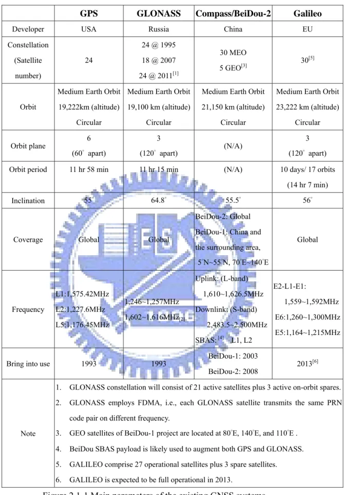
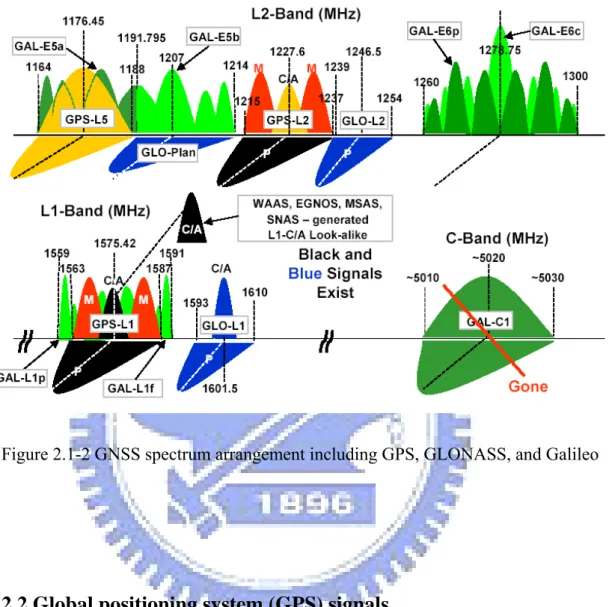
The main parameters of the GNSS system are shown in Figure 2.1-1, and the spectrum arrangement for the GPS, Galileo and GLONASS is shown in Figure 2.1-2.

GPS GLONASS Compass/BeiDou-2 Galileo

Developer USA Russia China EU

Constellation (Satellite number) 24 24 @ 1995 18 @ 2007 24 @ 2011[1] 30 MEO 5 GEO[3] 30 [5] Orbit

Medium Earth Orbit 19,222km (altitude)

Circular

Medium Earth Orbit 19,100 km (altitude)

Circular

Medium Earth Orbit 21,150 km (altitude)

Circular

Medium Earth Orbit 23,222 km (altitude) Circular Orbit plane 6 (60° apart) 3 (120° apart) (N/A) 3 (120° apart) Orbit period 11 hr 58 min 11 hr 15 min (N/A) 10 days/ 17 orbits

(14 hr 7 min)

Inclination 55° 64.8° 55.5° 56°

Coverage Global Global

BeiDou-2: Global BeiDou-1: China and the surrounding area,

5°N~55°N, 70°E~140°E Global Frequency L1:1,575.42MHz L2:1,227.6MHz L5:1,176.45MHz 1,246~1,257MHz 1,602~1,616MHz[2] Uplink: (L-band) 1,610~1,626.5MHz Downlink: (S-band) 2,483.5~2,500MHz SBAS:[4] L1, L2 E2-L1-E1: 1,559~1,592MHz E6:1,260~1,300MHz E5:1,164~1,215MHz

Bring into use 1993 1993 BeiDou-1: 2003

BeiDou-2: 2008 2013 [6]

Note

1. GLONASS constellation will consist of 21 active satellites plus 3 active on-orbit spares. 2. GLONASS employs FDMA, i.e., each GLONASS satellite transmits the same PRN

code pair on different frequency.

3. GEO satellites of BeiDou-1 project are located at 80°E, 140°E, and 110°E . 4. BeiDou SBAS payload is likely used to augment both GPS and GLONASS. 5. GALILEO comprise 27 operational satellites plus 3 spare satellites.

6. GALILEO is expected to be full operational in 2013.

Figure 2.1-2 GNSS spectrum arrangement including GPS, GLONASS, and Galileo

2.2 Global positioning system (GPS) signals

2.2.1 Legacy GPS signals

GPS reached full operational capability in early 1995, the 24 satellites originally broadcast ranging codes and navigation data on two frequencies using CDMA technique; that is, there are only two frequencies in use by the system, called L1 (1.575.42 MHz) and L2 (1,227.6 MHz). Each satellite transmits on these frequencies, but with different ranging codes than those employed by other satellites. The Gold code is selected because of its low cross-correlation properties. Each satellite generates a short code referred to as the coarse/acquisition (C/A) code and a long code denoted as the precision or P(Y) code. The navigation data provides the means for the receiver

to determine the location of the satellite at the time of signal transmission, whereas the ranging code enables the user’s receiver to determine the satellite (i.e., propagation) time of the signal and thereby determine the satellite-to-user range.

The L1 frequency is modulated by two PRN codes (plus the navigation message data), the C/A code, and the P code. The L2 frequency is modulated by only one PRN code at a time. The C/A code has a chipping rate of 1.023 Mchips/s and the P code has a chipping rate of 10.23 Mchips/s. The P code is modulated in phase quadrature with the C/A code on L1. The P code signal is 3-dB low relative to the C/A code on L1. The legacy L1 signals can be represented as follow.

L₁(t)=A[P(t)⊕D(t)]cos(ωt)+ 2A[C(t)⊕D(t)]sin(ωt) (2.2.1-1)

where, A denotes amplitude, denotes P code, denotes navigation data, and C denotes C/A code.

) (t

P D(t)

2.2.2 Modernized GPS signals[3]

In January 1999, the U.S. government announced a new GPS modernization initiative that called for the addition of two civil signals to be added to new GPS satellites. These signals are denoted as L2C and L5. The L2C signal is at the L2 frequency; the L5 signal resides in ARNS band at 1,176.45 MHz. These additional signals will provide civil, commercial and scientific users the ability to correct for ionospheric delays by making dual frequency measurement, thereby significantly increasing civil user

1). L2 civil signal

The L2 civil (L2C) signal has a similar power spectrum (i.e., 2.046 MHz null-to-null bandwidth) to the C/A code. However, the L2C uses two different PRN codes per satellite. The first PRN code is referred to as the civil moderate (CM) code which employs a sequence that repeats every 10,230 chips. The second code, the civil long (CL) code, is extremely long with a length of 767,250 chips. These two codes are generated each at a 511.5 kchip/s rate. The CM code is modulated by a 25-bps navigation data stream. The baseband L2C signal is formed by the chip-by-chip multiplexing of the CM (with data) and the CL codes. Hence the L2C signal has an overall chip rate of 2 × 511.5 kchip/s rate = 1.023 Mchip/s, which account for its similar power spectrum to the C/A code.

2). L5 signal

L5 signal uses QPSK modulation to combine an in-phase signal component (I5) and a quadraphase signal component (Q5). Different PRN codes with same length-10,230 are used for I5 and Q5. The I channel is the data channel and the Q channel is the pilot (no data) channel. I5 is modulated by 50-bps navigation data. A 10.23 MHz chipping rate is employed for both the I5 and Q5 PRN codes resulting a 1-ms code repetition period.

3). M code

During the mid to late 1990s, a new military signal called M code was developed for the military users. This signal will be transmitted on both L1 and L2 and is spectrally separated from the GPS civil signals in those bands. The spectral separation permits the use of non-interfering higher power M code modes that increase resistance to interference. The M code is intended to eventually replace the P(Y) code.

The new M code employs binary-offset-carrier (BOC) modulation. Specifically, M code is a BOC (10, 5) signal. The first parameter denotes the frequency of a

square-wave subcarrier, which is 10 × 1.023 MHz, and the second parameter denotes the M code generator code chipping rate, which is 5 × 1.023 Mchip/s.

2.3 GPS receiver

1) Receiver structure[4]

The structure of a typical GPS receiver is shown in Figure 2.3-1. The signal transmitted from the GPS satellites are received from the antenna. Through the RF chain the input signal is amplified to proper amplitude and the frequency is converted to a desired IF frequency. An analog-to-digital converter (ADC) is used to digitize the output signal. The antenna, RF chain, and ADC are the necessary hardware used in the receiver.

After the signal is digitized, a software approach can be taken to perform the

subsequent processes. The Acquisition is to find the signal of a certain satellite. The Tracking program is used to find the phase transition of the navigation data. In a conventional receiver, the Acquisition and Tracking are performed by hardware. From the navigation data phase transition, the subframes and navigation data can thus be obtained. Ephemeris data and pseudoranges can be obtained from the navigation data. The ephemeris data are used to obtain the satellite position. Finally, the user position can be calculated from the satellite positions and the pseudoranges.

2) Signal-to-Noise Ratio (SNR) [10]

The L1 C/A code signal is transmitted at a minimal level of 478.63W (26.8 dBW) effective isotropic radiated power (EIRP). The free-space loss factor (FSLF) is given

by )2 4 ( R FSLF π λ =

where, R is the distance between GPS satellite and the receiver, λ is the wavelength. Using R=2×107 and λ=0.19m at L1 frequency, the FSLF is about -182.4 dB.An

r d to be isotropic, then the rec

has about 3 dB of gain, the

z, and is the r a GPS receiver is 513 K, resulting in a nois

ried in noise. In this thesis, we will cus the analysis on low SNR environments as of around -20 dB.

oftware receivers have drawn more and more attention because of their flexibility to transmissions and the removal of several analog

bits additional atmospheric loss factor (ALF) is about 2 dB, and if the eceiving antenna is

assume eived signal power is

EIRP-FSLF-ALF=26.8-182.4-2=-157.6 dBW. Since a typical GPS antenna with right-hand circular polarization and a hemispherical pattern

result of minimum received signal power is -157.6+3= -154.6 dBW.

The noise power in the first RF amplifier stage of the receiver front end is given by

B kT

N = _e , where, k =1.3806×10−23J/K , B is the bandwidth in H T_e

effective noise temperature in degree Kelvin. A typical effective noise temperature fo e power of about -138.5 dBW in a 2MHz bandwidth. As about 90% of the C/A-code power lies in a 2-MHz bandwidth, so there is only about 0.5 dB loss in signal power. Consequently, the SNR in a 2MHz

bandwidth is (-154.6-0.5)-(-138.5)= -16.6 dB.

Since the SNR is far below 0 dB, the signal is bu fo

3) Software-GPS Receiver (SGR) S

demodulate a number of distinct RF

components at RF band. When implementing a real-time SGR (Software-GPS

Receiver), owing to the correspondingly high sampling rate, 1 or 2-bits quantization is usually selected in order to reduce computation and storage load. However, few quantization may induce significant degradation[2] [5]. An improved tracking structure called post-correlator phase compensation (PCPC) structure and a novel carrier phase discriminator called noise-balanced digital phase discriminator (NB-DPD) are proposed in the thesis.

3. Tracking Loop in One-bit Software-GPS Receiver (SGR)

3.1 Conventional tracking loop

The tracking of a GPS receiver consists of the code tracking and carrier tracking loops, which locks onto and tracks the PRN code and carrier of the GPS satellite signal respectively. A typical tracking structure is shown in Fig 3.1-1.

Fig 3.1-1 combined code and carrier tracking loop

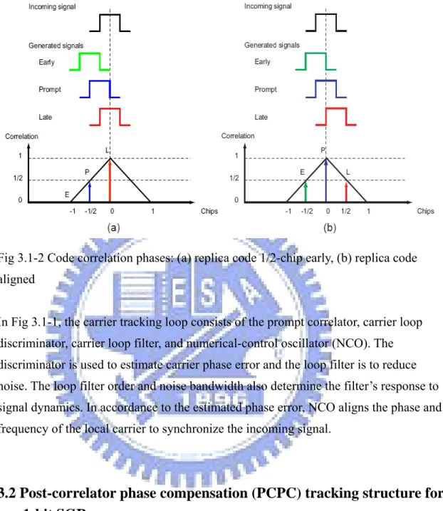
For the code tracking, the delay-lock-loop (DLL) is used to make the

receiver-generated code line up with incoming code precisely. In Fig 3.1-1, three different replica code phases, early, prompt, and late, for both I- and Q-channels are correlated simultaneously with the same incoming signal. The early and late codes respectively lead and lag the prompt code by less than 0.5 code chips and always maintain these relative positions.[10] In normal operation the prompt code is aligned with the code of the incoming signal so that the squared magnitude of the prompt correlator output is at the peak of the cross-correlation function, and the output magnitude of the early and late correlators have smaller but equal values on each side of the peak. Fig 3.1-2 shows the early, prompt, and late envelopes as the phases of the replica code signals are advanced/ aligned with respect to the incoming signals.

2 2

P P Q

Fig 3.1-2 Code correlation phases: (a) replica code 1/2-chip early, (b) replica code ligned

Fig 3.1-1, the carrier tracking loop consists of the prompt correlator, carrier loop iscriminator, carrier loop filter, and numerical-control oscillator (NCO). The iscriminator is used to estimate carrier phase error and the loop filter is to reduce oise. The loop filter order and noise bandwidth also determine the filter’s response to

signal dyna CO aligns the phase and

equency of the local carrier to synchronize the incoming signal.

r

a In d d n

mics. In accordance to the estimated phase error, N fr

3.2 Post-correlator phase compensation (PCPC) tracking structure fo

1-bit SGR

3.2.1 Problem description

Firstly, let’s consider the quantization effect on the conventional carrier tracking loop. For SGR, we have pre-established sine table and cosine tables given by

) 2 cos( ) ( s I n fnT LO = π ) 2 sin( ) ( s Q n fnT LO = π

where is the local carrier frequency and is the sampling period. The tables suall e very few bits per sample in order to save computation and storage. For -bit ADC SGR, the received data and the local carrier are quantized as two alues given by f y us s T u ) (n S 1 v

(

cos(2 )

)

sgn ) ( s I n fnT LO = π

(

sin(2 )

)

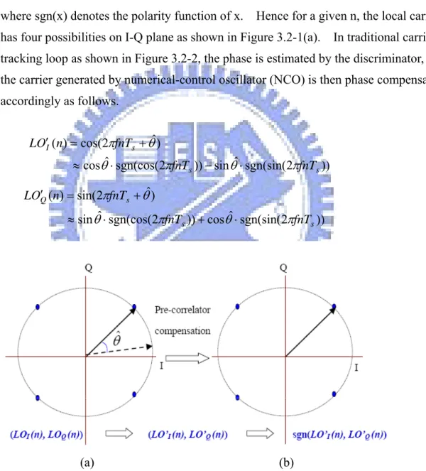
sgn ) ( s Q n fnT LO = π ,

here sgn(x) denotes the polarity function of x. Hence for a given n, the local carrier as four possibilities on I-Q plane as shown in Figure 3.2-1(a). In traditional carrier

acking loop as shown in Figure 3.2-2, the phase is estimated by the discriminator, and e carrier generated by numerical-control oscillator (NCO) is then phase compensated ccordingly as follows. w h tr th a ( I O L ′ )) 2 sgn(sin( ˆ sin )) 2 sgn(cos( ˆ cos ) ˆ 2 cos( ) s s s fnT fnT fnT n π θ π θ θ π ⋅ − ⋅ ≈ + = )) 2 sgn(sin( ˆ cos )) 2 sgn(cos( ˆ sin ) ˆ 2 sin( ) ( s s s Q fnT fnT fnT n O L π θ π θ θ π ⋅ + ⋅ ≈ + = ′ (a) (b)

Figure 3.2-1 Schematic plot for pre-correlator phase compensation tracking loop

In order to compute efficiently, the multiplication between and local carrier is achieved by bitwise processing such as XOR operation. Hence the compensated

CO signals and

) (n

S

,LO_I′(n) LO_Q′ (n), are quantized as follows.

))) 2 sgn(sin( ˆ sin )) 2 sgn(cos( ˆ sgn(cos )) ( sgn( ) ( _{I s s} I n LO n fnT fnT O L ′′ = ′ = θ π − θ π ))) 2 sgn(sin( ˆ cos )) 2 cos( sgn(sin )) ( sgn( ) ( _{Q s s} Q n LO n fnT fnT O L ′′ = ′ = θˆsgn( π + θ π

The signal constellation on I-Q plane after phase compensation is shown in Figure 3.2-1(b). From Figure 3.2-1, the phase ambiguity of local carrier is π/2 (±π/4) because we only have 4 possibilities on I-Q plane. Similarly, as we have m-bit ADC carrier

ble for pre-correlator phase compensation structure in SGR, the resultant phase ta ambiguity is given by ⎟ ⎠ ⎞ ⎜ ⎝ ⎛± = ₊₁ 2 2m m amb π π θ

Hence the degradation on the magnitude of in-phase correlator output is given by

) ( 2 cos log 10 ₁₀ dB n Degradatio amb ⎟ ⎠ ⎞ ⎜ ⎝ ⎛ = θ

The fewer bits we use, the more degradation we suffer because of the quantization effect.

Figure 3.2-2 Simplified pre-correlator phase compensation tracking loop Input data

Σ

NCO Carrier Phase Discriminator

Σ

θ

ˆ

P

I

P

Q

) (n S ) (n Q ) (n I′′ O L _{L ′O′} ) (n LOQ ) (n LOI Code Gen.

3.2.2 The Proposed PCPC structure

order to resolve the phase ambiguity problem induced by few-bits quantization, we

oid uity induced by few bits quantization.

ence the proposed structure is called post-correlator phase compensation (PCPC) structure and the phase can be compensated accurately as shown in Figure 3.2-4. In order to investigate the features of PCPC structure, we categorize components after

hase discriminator into three groups as follows. In

propose a structure as shown in Figure 3.2-3, where Figure 3.2-3(a) is a simplified version and the Figure 3.2-3(b) is a complete system structure. Compared with the traditional one as in Figure 3.2-2, the proposed structure compensates the correlator output of I-channel with the estimated carrier phase after correlators in order to av significant phase ambig

H

p

Input

Figure 3.2-3(a) Simplified post-correlator phase compensation (PCPC) tracking loop

data

Σ

NCO Code Gen. Carrier Phase Discriminator

Σ

θ

ˆ

P

I ′

P

I

P Q

)

n

S

) (n LO_Q ) n LO

(

( I

Figure 3.2-3(b) Implemented post-correlator phase compensation (PCPC) tracking loop

Group G1 (phase-rotation part): The phase rotation in every observation interval is due to frequency offset and the beginning phase offset of pre-established carrier table. G1 includes a high-pass-filter H1 and a low-pass-filter H2. The phase-rotation

component of input signal is extracted through H1. The implemented frequency response of H1 is given by

(3.2-1)

Then H2 suppresses disturbances such as noise. The frequency response of H2 is given by . 1 ) ( 1 1 − − = z z H 1 2 1 ) ( ₋ − = az b z H (3.2-2)

The output of H2 can be used further to estimate frequency variation such as Doppler shift or carrier frequency bias, and hence the frequency-lock-loop (FLL) is achieved. Note t

compensated as well so that an accurate frequency estimate is obtained.

Group G2 (loop filter part): G2 acts as the loop filter and handles the phase-error component of the output of phase discriminator. The implemented frequency response of a 2nd order loop filter is given by

hat phase offset induced by carrier table as shown in Figure 3.2-5 must be

. 1 ) ( 2 ₁ 1 3 = + ₋ − z k k z H (3.2-3)

Group G3 (phase estimate): G3 combines the phase-rotation part and the phase-error component. The estimated phase is then obtained. The implemented frequency response of the filter H4 is given by

1 1 4 1 ) ( ₋ − − = z z z H (3.2-4)

Finally, the in-phase output is compensated as follows:

(3.2-5) P I ⎥ ⎦ ⎤ ⎢ ⎣ ⎡ = ′ P P O O P Q I I [cos(θˆ ) sin(θˆ )]

3.2.3 Analysis

The analysis of analog PLL has been well established for decades [7][8]. In the f we analyze the proposed carrier tracking structure based on digital approach, whi more appropriate for SGR.

ollowing, ch is

Suppose the received data is given by

], [' ' ]) [ 2 cos( ] [ ] [ ] [ 0 n D nC n f nT n u n S = π c s +φ +

where, D[n] is navigation data, C[n] is PRN code and u” [n] is additive white Gaussian noise. Suppose that local PRN code Cˆ n[ ] perfectly matches C[n]. Then

], [' ]) [ 2 cos( ] [ ] [ 1 n D n f nT n u n S = π _{c s} +φ + where ]), [ 2 sin( ] [ ' ]) [ 2 cos( ] [ ' ] [ ˆ ] [' ' ] [' n fnT n u n fnT n u n C n u n u s Q s I π +φ + π +φ = =

and u' n_I [ ] and u' n_Q[ ] are real part and imaginary part of u['n], respectively.

Suppose the local carrier are given by

) 2 cos( ] [ _s I n fnT LO = π , ) 2 sin( ] [ s Q n fnT LO = π .

As we use pre-established carrier table which contains the data for n=0,1,2…N-1, i. e. the beginning phase of data is always zero. However, the initial phase of each re data may be not zero and change from

, ceived interval to interval. Hence the true local carrier should incorporate a correct offset given by

) 2 cos( ] [n fnT k LO_I = π _s − Φ_{LO ,} ) 2 sin( ] [ _{s LO} Q n fnT k LO = π − Φ ,

where Φ_LO =2 fTπ mod2π, T is the observation period, and

⎥⎦ ⎥ ⎢ n

⎣ ⎦

x ⎢⎣ = N k , where is

a function rounding x to the greatest smaller integer, and N is the total samples within . After demodulation, we have

T

[

]

, ] [ sin ] [' ] [ cos ] [' ] [ cos ] [ 1 ]) [ 2 sin( ] [' ]) [ 2 cos( ] [' ]) [ 2 cos( ] [ ) 2 cos( 2 ] [ ] [ 2 ] [ ₁ 1 ) 1 ( n S n LO N k I k N Nk n I ⋅ =

∑

+ − = 1 ) 1 ( 1 ) 1 ( terms frequency high n n u n n u n n D N n nT f n u n nT f n u n nT f n D k fnT Q I k N Nk n s c Q s c I s c k N + Φ + Φ + Φ = + + + + + ⋅ Φ − =

∑

∑

− + = − + φ π φ π φ π π N _n=Nk s LO where ] [ 2 ] [n = πΔfnTs +kΦLO +φ n Φ ( .2-6) 3 and Δf = fc − f constan

. As we neglect high frequency part after integration and assume that t over

] [n

D are [kT,(k+1)T)=[kNTs,(k+1)NTs), i. e.,

where n = Nk, Nk+1, Nk+2…N(k+1)-1, and then

] [' ] [n D k D = , ] [' ' sin ] [ ] [' cos ] [ ] [' cos ] [' ] [k D k k u k k u k k I = Φ + I Φ + Q Φ (3.2-7) e wher ,] [ cos 1 N(k+1)−1 ] [' cos

∑

= Φ = Φ Nk n n N k (3.2-8) .] [ sin 1 ] [' ' sin 1 ) 1 (

∑

+ − = Φ = Φ N k Nk n n N k (3.2-9) ,] [ cos ] [' ] [' cos ] [

∑

= Φ = Φ Nk n I I u n n N k k u 1 1 ) 1 (k+ − N ]. [ sin ] [' 1 ] [ sin ] [ 1 ) 1 ( n n u N k k u k N Nk n Q Q Φ ′′ =

∑

Φ − + =

Similarly, we have the quadrature term

]. [' cos ] [ ] [' ' sin ] [ ] [' ' sin ] [' ] [k D k k u k k u k k Q = Φ + I Φ − Q Φ (3.2-10)

] [' ' sin ] [ ] [' cos ] [ ] [' cos ] [' ] [' cos ] [ ] [' ' sin ] [ ] [' ' sin ] [' tan ˆ 1 k u k k D k k u k k u k k D I Q I + Φ Φ − Φ + Φ = Φ − ] [ ] [ tan ] [ 1 k k u k k I k Q k Q Φ + Φ = − (3.2-11)

. As we neglect noise effect, from Eq. (3.2-6), Eq (3.2-8) and Eq (3.2-9), we have Suppose ]Φ['k]=Φ' ['k ], [ 2 ] [' ] [ ˆ k k fkT k k LO φ πΔ + Φ + = Φ = Φ (3.2-12)

From Eq. (3.2-12), the phase discriminator Φˆ k[ ] consists of three components: (i) 2πΔfkT: frequency offset component,

(ii) : the beginning phase offse ii)

LO

kΦ t error of pre-established carrier table,

] [k

φ

(i : phase error component.

The f ponent changes very slowly comp

re as shown in Figure 3.2-3(b), the utput of H1 is given by

requency offset com ared with the phase error component. As we implement FLL in PCPC structu

o ]. 1 [ ] [ 2 ] 1 [ ˆ ] [ ˆ ] [ 1 − − + Φ + Δ = − Φ − Φ = k k fT k k k O_H LO φ π (3.2-13) Since φ ] 1 [ ] [k − kφ −

φ can be regarded as a high freque after LPF H2, the output of H2 is given by

ncy term and would be removed

LO

H k fT

O ₂[ ]=2πΔ +Φ (3.2-14)

From Eq. (3.2-14), the estimated frequency adjustment is given by

T k O fˆ = H2[ ]−ΦLO Δ . ( π 2 3.2-15)

e utilize Eq. (3.2-15) to adapt local carrier frequency as shown in Figure 3.2-3(b). W

The frequency response of the proposed structure after phase discriminator is characterized by

(

)

[

( ) ( ) ( ) ( ) ( ) ( )

]

( ) ) ( _{3 1 2} 4 z z z H z z H z H z z H θi −θo +θi =θo (3.2-16)

rom Eq. (3.2-16), the overall system response is given by F

[

]

) ( ) ( 1 ) ( ) ( ) ( ) ( ) ( ) ( ) (z 4 3 2 1 3 4 0 z H z H z H z H z H z H z H z i + = = θ θ +

[

]

] ) 1 ( ) 2 ( 1 )[ 1 ( ) ( ) 2 ( 2 1 1 2 1 1 2 1 1 2 1 1 2 1 1 − − − − − − − + − + + − + + + + + − + + = z k z k k az z b ak z ak ak k b k k b z (3.2-17) e choose satisfying a |a|<1

W , and select and carefully so that all the poles (z) fall guarantees the stability of the system.

.2.4 Implementation issues

output of H2 can be used to estimate frequency variation irectly. The sources of frequency variation include motion of satellite or user, clock drift and local carrier frequency bias etc. It is

effect of local carrier table must be considered in order to attain correct frequency ariation. The effect is induced because the beginning phase of a pre-established

n interval may be not the multiple of arrier wavelength. A schematic plot of this effect is shown in Figure 3.2-5.

1

k k₂

of H in the unit circle. This condition

3

1) FLL scheme:

As mentioned above, the d

worth to mention that the phase offset

v

carrier table is always zero while the local carrier of the following interval may have a nonzero beginning phase, i.e., the integratio

) Range of phase for each stage:

is implemented after ATAN phase detector, the phase nge of each stage must be taken care carefully in order to avoid navigation bit

d 2π transition influence on phase estimate.

Figure 3.2-5 An example of the beginning phase offset problem for a pre-established carrier table with integration interval 1 ms

2

Since the phase compensation ra

4. Carrier Phase Discriminator

As the feasible PCPC structure for 1-bit SGR is provided in the previous section, we are ready to propose a computationally efficient phase discriminator as follows.

4.1 Conventional phase discriminators

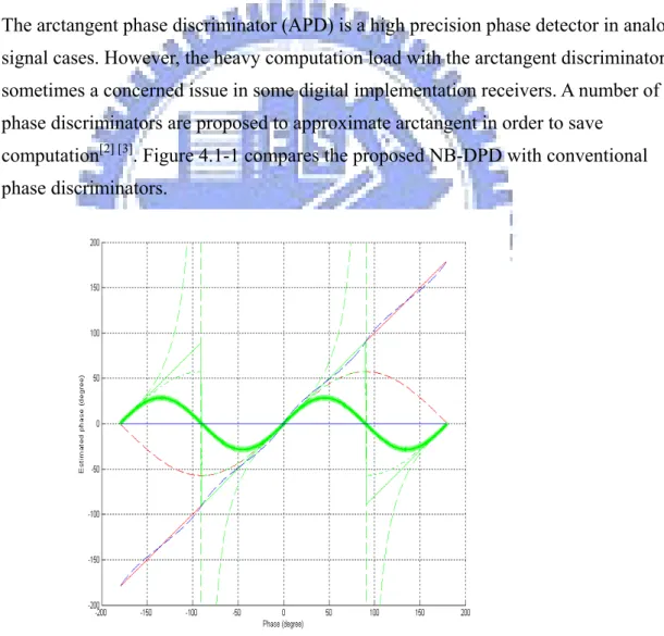
The arctangent phase discriminator (APD) is one of the most widely used in PLL tracking loops since it’s an optimal detector in analog signal cases with

additive-white-Gaussian-noise (AWGN).[9].

The arctangent phase discriminator (APD) is a high precision phase detector in analog signal cases. However, the heavy computation load with the arctangent discriminator is sometimes a concerned issue in some digital implementation receivers. A number of phase discriminators are proposed to approximate arctangent in order to save

computation[2] [3]. Figure 4.1-1 compares the proposed NB-DPD with conventional phase discriminators.

Figure 4.1-1 Comparison of ATAN2 (red solid) with ATAN (green solid), Qp (red dashed), Qp/Ip (green dashed), sign(Ip)Qp (green dash-dotted), IpQp, (green starred) and NB-DPD (blue dashed) without noise.

Another issue with arctangent is the quantization loss. When applying arctangent in igital cases with few bits ADC, the accuracy will degrade greatly due to high

iscriminator has been shown to achieve much higher accuracy than the arctangent p to several orders in high SNR cases. owever, the DPD does not perform well in low SNR environments such as global

ise. DPD), which s is proposed in the following sections. d

quantization loss. A novel phase discriminator, called digital phase discriminator (DPD), is proposed to mitigate quantization loss by Chang and Kao[1]. The DPD d

discriminator in 1-bit software-defined receiver u H

navigation satellite system (GNSS) applications because of its sensitivity to the no A modified DPD, called noise-balanced digital phase discriminator

4.2 Proposed noise-balanced digital phase discriminator (NB-DPD)

Figure. 4.2-1. Schematic plot of the system

A schematic plot of the system is shown in Figure 4.2-1. First, consider the transmitted signal given by ) 2 sin( ) (t = A πft+θ s c (4.2-1)

where f c is the carrier frequency, and the received signal is given by

) ( ) 2 sin( ) (t A f t u t r = πc +θ + (4.2-2) where u(t) is the environmental noise. In noiseless environments, the output signal of 1-bit ADC is given by

]] [ sgn[ )] ( sgn[ ] 2 sgn[sin( ] [n fnT s nT s n x = πc s+θ) = s = (4.2-3) where is the sampling period and sgn(·) denotes the polarity function, i. e., sgn[x] = 1 if x 0 and sgn[x] = −1 if x

s

T

≥ ≤ 0. We can treat sgn[ ] as a square wave and x[n] as samples on this square wave. Similarly, in noisy environments, the output signal of 1-bit ADC is given by

(4.2-4) ) (t s ]] [ ] [ sgn[ ] [n sn u n y = +

Figure 4.2- 2. The block diagram expressing noiseless channel and noisy channel

Figure 4.2-3. Binary probability model

be explained in Figure 4.2-2. In order to analyze the DPD in noisy environments, we need to establish the connection between x[n] and y[n]. This can be achieved through probability approach. First, we ha al probabilities:

The overall system can

ve the following condition

1 ] [ ( 00 P y n =− P = | 1x[n]=− ) (4.2-5) 1 ] [ ( 01=P y n = P | )[ ] 1 , − = n x , (4.2-6) 1 ] [ ( 10=P y n =− P | 1x[n]= ) , (4.2-7) 1 ] [ ( 11=P y n = P | )x[n]=1 , (4.2-8)

sing Eqs.(4.2-5)-(4.2-8), the binary probability model is established as shown in Figure 4.2-3. Next, we consider u(t) as a zero-mean additive white Gaussian noise (AWGN), it is reasonable to assume that

, P01=P10 < 2 1 11 00 P P = _(4.2-9)

With Eq. (4.2-9), the probability model in Figure 4.2-3 becomes a binary symmetrical structure. Hence the proposed modified DPD is called noise-balanced digital phase discriminator (NB-DPD), which assumes the noise effect is “balanced” regarding in-phase channel and quadrature channel at every sample of the incoming signal.

Furthermore, similar to the digital perspective in Eq. (4.2-3), we also regard local reference signals as samples on square wave given by

)] 2 sgn[sin( ] [ s I n f nT LO = π _ω , (4.2-10) )] 2 sgn[cos( ] [ s Q n f nT LO = π_ω , (4.2-11)

where is the local carrier frequency. From the Eq. (4.2-3) ~ Eq. (4.2-11), the NB-DPD model is provided in Figure 4.2-4.

Figure 4

hase

u[n]

ω

f

.2-4: The NB-DPD signal model

The DPD approach is based on digital perspective, which derives received carrier p by comparing the time delay between received signal and local reference signal as shown in Figure 4.2-5. s[n] NCO In x[n] y[n] LO n] + I [ + Σ I s(t) θˆ + + Q LOQ[n] Σ x’[n] y’[n] Qn

Figure 4.2-5: The schematic plot of time delay and corresponding phase difference θ etween the received signal an al refe nce signals in (a) in-phase channel and (b) uadrature channel, respectively.

et T be the tion time and N = T/Ts be the number of samples within T. Assume and b d loc re q L observa ω f fc = φn =2πfcnTs, where n = 0, 1, 2..., N−1. we have ]] [ ] [ sgn[ ] [n x n u n y n + I , (4.2-12) (4.2-13) (4.2-14) ) = = sgn[ ] [n x y Qn= ′ = ′[n]+u[n]],

∑

∑

− = − = N 1I N 1y[n] I = =0 n 0 n n

∑

∑

− = − = ′ = = 1 0 1 0 ] [ N n N n n y n Q Q (4.2-15

Let N+ denote the number of samples with = 1, N− denote the number of samples

with = −1, denote the number of sam les with = 1 and denote the num sam les with = −1. Then we have

n I p n I ber of + ′ N p n Q N₋′ n Q , Q=N₊′ −N₋′ − + − = N N I (4.2-16)

Suppose the observed samples satisfy the uniformity condition, i. e., , φ₁, · · · , φN₋₁

ase e 0

φ

are uniformly distributed over [0, 2π].[1] Firstly let’s consider the c at the ph differenceθ is in the range of [0,π/2], i.e., 0≦θ<π/2. W

delay between the received signal and local reference signal

and the binary probability model as in Figure 4.2-3, we have and for I-channel as follows

ase th

ith respect to the tim as shown in Figure 4.2-5 − N N₊ 10 01) ( ) 1 ( P NP N N π θ π π θ − + − = − ⎥⎦ ⎤ ⎢⎣ ⎡ − + =N Pe π θ π π θ 2 , (4.2-17) 01 10) 1 ( P NP N N π θ π θ π + − − = + ⎥⎦ ⎤ ⎢⎣ ⎡ − + − =N Pe π π θ π θ π 2 , (4.2- 8) 1

where, Pe = P10 = P01. Similarly, for Q-channel, we have

10 01 ) 2 2 π 1 ( ) 1 ( ) 1 ( ' N P NP N θ π θ + + − − = , − ⎥⎦ ⎤ =N_⎢⎣⎡ − + 2θ Pe , ( π π θ ) 2 1 ( 4.2-19) ) 1 ( ) 2 1 ( ) 2 1 ( ' NP01 N N+= − + + π θ θ 10 P − , π ⎥ ⎤ e P π θ 2 . (4.2-20) ⎦ ⎢⎣ ⎡ _{+ −} = N π θ ) 2 1 (

From Eqs.(4.2-16)-(4.2-20), we have ) 2 1 )( 2 ( Pe N N − = − − = + π θ π , (4.2-21) N I − ) 2 1 ( 2N − = ′ − ′ = N N Pe Q + − π θ , (4.2-22)

Combining Eq. (4.2-21) and Eq. (4.2-22), we obtain

π θ 2 1− = + Q I I ( .2-23)

As for other phase ranges of

4 θ, we have when π/2≤θ <π, π θ 2 1− = + Q I I (4.2-24) when −π ≤θ <0, π θ 2 1+ = + Q I I (4.2-25)

From Eq. (4.2-23), (4.2-24) and (4.2-25), we have

) 1 ( 2 I Q I + − =π θ (4.2-26)

s for the polarity ambiguity of

A θ, it can be resolved by

[ ]

sgn

[ ]

Q

sgnθ = (4.2-27) which is obtained from Eq. (4.2-22). Hence we have

[ ]

(1 ) 2 sgn ˆ Q I I Q + − = π θ (4.2-28)

Note that the phase estimate in Eq

he above approach is developed in a more intuitive way and can be verified by the probabilistic approach in [11].

. (4.2-28) does not depend on noise.

4.3 Analysis of NB-DPD estimator

Recall the signals and parameters as follows.

1) Received signal and local carriers: ) ( ) 2 sin( ) (t A f t u t r = πc +θ + ) 2 sin( ) (t f t LO_I = π _ω ) 2 _ω cos( ) (t f t LO_Q = π m

2) After 1-bit ADC:

e fc= f_ω and φn=2πfcnTs, ]n∈[0,N−1 ,N

Assu is the number of total samples

in observation period, then we have:

)] ( ) sin( sgn[ )] ( sgn[r nT_s = A φ_n+θ +u nT_s )] sgn[sin( )] ( sgn[LO_I nT_s = φ_n )] sgn[cos( )] sgn[LO (nT_{Q s} = φ_n 3) Correlator output: )] ( sgn[ )] ( sgn[ _{s I s} n r nT LO nT I = ⋅ sgn[sin( )] ( ) sin( sgn[A φ_n +θ +u nT_s ⋅ _n)] = φ )] ( sgn[ )] _{Q s} s ( sgn[ n r nT LO nT Q = ⋅ )] sgn[cos( )] ( ) sin( sgn[A φ_n +θ +u′ nT_s ⋅ φ_n = 4) SNR and σ :

denotes the standard deviation of u(nT_s) σ 2 2 2σ A SNR= SNR A = ⇒σ 2

4.3.1 Statistical properties of I andn Qn

[11]

and variance of the random variables and are derived below.

4.3.1.1

1). when

The prabability-density-function (pdf), mean,

I_n Q _n n I , we have sin(φn)≥0 ) , 0 [ π φn∈ (a) Conditional pdf: ) 1 (In = P θ =P(sin(φ_n+θ)+u(nT_s)≥0θ) )) sin( 2 ( 1 ) ) sin( ( 1 φ θ σ θ φ + ⋅ − = + ⋅ − = A n Q Q SNR _n (4.3.1-1) ) 1 (In =− θ P =Q( 2SNR⋅sin(φ_n +θ)) _(4.3.1-2) ) Mean: (b ) 1 ( 1 θ μIn = ×P In = −P(In =−1θ) =1−2Q( 2SNR⋅sin(φn +θ)) (4.3.1-3) (c) Variance: 2 2 2 _{[ ]} n n n I I E I μ σ = − _{=4Q( 2SNR⋅sin(φn +θ))−4[ ( 2 ⋅sin(φ +θ))]}2 n SNR Q ⋅ + ⋅ =4Q( 2SNR sin(φ_n θ)) [1−Q( 2SNR⋅sin(φ_n+θ))] (4.3.1-4)

2). when φn∈[−π,0), we have sin(φn)≤0 (a) Conditional pdf: ) 1 (In = θ P =P(sin(φ_n+θ)+u(nT_s)≤0θ) )) sin( 2 ( ⋅ φ +θ =Q SNR _n (4.3.1-5) ) 1 (In =− θ P =1−Q( 2SNR⋅sin(φ_n +θ)) _(4.3.1-6) (b) Mean: ) 1 ( 1 θ μ_I = ×P I_n = n −P(In =−1θ) =−1+2Q( 2SNR⋅sin(φn +θ)) (4.3.1-7)

(c) Variance: 2 2 2 _{[I ]} E μ σ = − _{=4 ( 2 ⋅sin(φ +θ))−4[ ( 2 ⋅sin(φ +θ))]}2 n SNR Q Q SNR _n n n n I I ⋅ + [1−Q( 2SNR⋅sin(φ_n +θ))] ⋅ =4Q( 2SNR sin(φ_n θ)) (4.3.1-8) -function is given by where Q dx z Q = 2 ) ( e z x

∫

∞ −2 2 1 π 4.3.1.2 1). when n Q ) 2 , 2 [ π π φn∈ − , we have cos(φn)≥0 (a) Conditional pdf: ) 1 (Qn = θ P =P(sin(φ_n +θ)+u′(nT_s)≥0θ) )) sin( 2 ( 1 ) ) sin( ( 1 φ θ σ θ φ + _{= − ⋅ +} ⋅ − = n _n SNR Q A Q (4.3.1-9) ) 1 (Qn =− θ P =Q( 2SNR⋅sin(φ_n +θ)) ( 3.1-10) (b) Mean: 4. ) 1 ( =− θ −P Q_n =1−2Q( 2SNR⋅sin(φ_n +θ)) ) 1 ( 1 θ μ_Q = ×P Q_n = n (4.3.1-11) ) Variance: (c 2 2 2 _{[ ]} n n n Q Q E Q μ σ = − _{=4Q( 2SNR⋅sin(φn +θ))−4[ ( 2 ⋅sin(φ +θ))]}2 n SNR Q ⋅ + ⋅ =4Q( 2SNR sin(φ_n θ)) [1−Q( 2SNR⋅sin(φ_n+θ))] (4.3.1-12) 2). when or ) 2 , [ π π φn∈ − − ) , 2 [π π φn∈ , we have cos(φn)≤0 (a) Conditional pdf: ) 1 (Qn = θ P =P(sin(φ_n +θ)+u(nT_s)≤0θ)

)) sin( 2 ( ⋅ φ +θ =Q SNR _n (4.3.1-13) ) 1 (Qn =− θ P =1−Q( 2SNR⋅sin(φ_n +θ)) _.3.1-14) ) Mean: (4 (b ) 1 ( 1 θ μQn = ×P Qn = − QP( _n =−1θ) =−1+2Q( 2SNR⋅sin(φn +θ)) (4.3.1-15) (c) Variance: 2 2 2 _{[ ]} n n n Q Q E Q μ σ = − _{=4Q( 2SNR⋅sin(φn +θ))−4[ ( 2 ⋅sin(φ +θ))]}2 n SNR Q ⋅ + ⋅ =4Q( 2SNR sin(φ_n θ)) [1−Q( 2SNR⋅sin(φ_n+θ))] (4.3.1-16) From Eq.(4.3.1-8) and Eq.(4.3.1-16), note that the variance of Inis same as Qn.

4.3.2 Statistical properties of and 1). and : Suppose i p Q groups i p I i p I i p Q P L K f f s

c = + _{, where is sampling rate,} s

f P> , P and L are relative L

prime integers. It can be shown that (φ₀,φ₁,...φ_p−1) are uniformly distributed over ] 2 , 0 [ π .[1] Define n p I I

i ={ n MOD P = pi} , Qpi ={Qn n MOD P = pi} , where,

1 0≤n≤ N− , 1i=0,1,2...P− , and p_i = .i i p Q Then (4.3 -1) 2). and Suppose we have the

group, and we have

components of

i

p

I group are i.i.d., and so are the components of

2 2 . .2 i p i p Q I σ σ = i Gp I i Gp Q M P N = ⋅ samples, Define

∑

− = = + ⋅ = 1 0 1 M m p mP n Gpi I i M I , (4.3.2-2)

∑

− = = + ⋅ = 1 0 1 M m p mP n Gpi Q i M Q , (4.3.2-3) (a) pdf: Let (4.3.2-4) (4.3.2-5) where k M I k I I i p i p i p _k p p M p M k b _⎟⎟ − − ⎠ ⎞ ⎜⎜ ⎝ ⎛ ≡ (1 ) ) , , ( k M Q k Q Q i p i p i p _k p p M p M k b _⎟⎟ − − ⎠ ⎞ ⎜⎜ ⎝ ⎛ ≡ (1 ) ) , , ( ) 1 ( = θ = i p p I P I p i , pQpi =P(Qpi =1θ) i (4.3.2-6) i , (4.3.2-7) ) (I_Gp x_k P i = ⇒ ( , , ) p I p M k b = ) (Q_Gp x_k P i = =b(k,M,pQp )

where M k 2 x_k =−1+ , k=0,1,2,....M (b) Mean: i p i i Gp I M m mP n Gp I I M E I E μ μ = = ⋅

∑

− = = + [ ] [ 0 (4.3.2-8) i i p p ]=E[I ]= 1 1 i p i i i i Gp p Q M m p mP n Gp Q Q E Q M E Q E μ μ = = ⋅

∑

− = = = = + ] [ ] 1 [ ] [ 1 0 (4.3.2-9) (c) Variance: s I i p ' are independent, ⇒ = 2 i Gp I σ M i p i p mP n I M m I 2 1 0 2 σ σ = ⋅

∑

− = = + ( M2 1 4.3.2-10) are inde s ' Q i p pendent, ⇒ = 2 Q σ i Gp M M i p p mP n Q M Q 1 2 2 1 _⋅

_∑

−_{σ =}σ + = i (4.3.2-11) m 2 0 = Since , (4.3.2-12)

(d) According to Central Limit Theorem (CLT), and approximate to Gaussian distribution when

N and 2 2 i p i p Q I σ σ = 2 2 i Gp i GP Q I σ σ = ⇒ i Gp I i Gp Q N is sufficiently large.i.e., ~ i Gp I ( , 2 ) i Gp i p I I σ μ ~N( , 2 ) i Gp i p Q Q σ μ when N →∞. i Gp Q

4.3.3 Statistical properties of I and Define Q

∑

− = ⋅ = 1 0 1 P p Gp i i I P I ,

∑

− = ⋅ = 1 0 1 P p Gp i i Q P Q (4.3.3-1) The range of , N k x=−1+2 , I and Q is x∈[−1,1] whe (a) pdf of re k∈[ N0, ], k is integer. I and

e and are independent, where

Q i Gp I j Gp I i≠ , we have j Assum ) ( ).... ( ) ( 1 ) 0 ω ω = Φ ⋅Φ Gp Gp I I P (4.3.3-2) ( 1 1 ω Φ − ω Φ p Gp I I ) ( ... ) ( ) ( 1 ) ( ₀ 0 ∗ = Gp Gp I I f i P i (4.3.3-3) 1 1 1 1 ∗ ∗ ₋ − ⇒ p p Gp Gp Gp I Gp I i f i f f

Similarly, assume d are in

ian dependent, we have Gp Q j Gp Q ) ( ).... ( ) ( ) ( 1 1 0 ω ω ω ω − Φ Φ ⋅ Φ = Φ p Gp Gp Gp Q Q Q Q P (4.3.3-4) 1 ) ( ... ) ( ) ( 1 ) ( = ∗ ∗ ⇒ f q f q q f q 1 1 1 1 0 0 ∗ Gp Gpp₋ p− Gp Gp Q Gp Q Gp Q Q f P (4.3.3-5)

(b) Assume and are independent, as well as and , where

i Gp I j Gp I i Gp Q j Gp Q i≠ . j

Since approximate to Gaussian distribution when is suff large, we have i Gp and I i Gp Q N iciently N(1 , 1 ) 1 0 2 2 1 0

∑

∑

− = − = p p I p p I i i Gp i i Gp P P μ σ N(μ_I,σ_I2), i.e., I ~ ~ I (4.3.3-6) N , i.e., N ~ Q (μ_Q,σ_Q2) Q~ (1 , 1 ) 1 0 2 2 1 0

∑

∑

− = − = p p Q p p Q i i Gp i i Gp P P μ σ (4.3.3-7)

From Eq.(4.3.3-6) and Eq.(4.3.37), note that σ_I2 and σ_Q2 are independent of θ. And from Eq.(4.3.2-12), since

(4.3.3-8) 2 2 i Gp i GP Q I σ σ = , we have 2 2 Q I σ σ =

4.3.4 Statistical properties of I and Q

Let Y = I , V = Q , then Yand are Ri (a) pdf:

(4.3.4-1)

(4.3.4-2)

Since ,

V cian distribution random variables.

⎩ ⎨ ⎧ < ≥ − + = 0 ; 0 0 ; ) ( ) ( ) ( y y y f y f y fY I I ⎩ v ⎨ ⎧ < ≥ − + = 0 ; 0 0 ; ) ( v v V ) ( ) (v f v f f Q Q N(μ_I,σ_I2), ~Q N(μ_Q,σ_Q2) , where, σ_I2 =σ_Q2, i.e., ∞ → N I ~ ) 2 ) ( exp( 2 1 ) ( ₂ 2 2 I I I I i i f σ μ πσ − − ⋅ = (4.3.4-3) ) 2 ) ( exp( 1 ) (q q f = ⋅ − ( 2 2 2 2 Q Q Q Q σ μ πσ − 4.3.4-4) ⎪ ⎪ ⎩ ⎪ ⎪ ⎨ ⎧ < ≥ ⋅ + − ⋅ = ⇒ 0 ; 0 0 ; ) cosh( ) 2 exp( 2 ) ( 2 2 2 2 2 y y y y y f I I I I I Y σ μ σ μ πσ _(4.3.4-5) ⎪ ⎪ ⎨ ≥ ⋅ − ) cosh( ) ; 0 2 ( _{2 2} 2 v Q Q V σ σ πσ _(4.3.4-6) ⎩ ⎪ ⎪ ⎧ < + ⋅ = 0 ; 0 exp 2 ) ( 2 2 v v v v f Q Q Q μ μ

(b) Mean:

oment of a Rician random [13] The m variable is given by

) 2 ; 2 1 ; 2 1 ( ) 2 1 ( ) 2 exp( ) 2 ( ] ₂ 2 1 1 2 2 2 2 σ μ π σ μ σ ⋅ + + [ Γ ⋅ − ⋅ = F k k k (4.3.4-7)

where, ) is the gamma function, and R E k (z Γ 1F1(α;β;γ) is the confluent hypergeometric function. , Γ(1/2)= π , Γ(3/2)= π /2 Since 1Γ(1)= , ) 2 2 2σ_I2 ; σ_I2 1 ; 1 ( ) exp( ) 2 ( 1 ] [ 2 _{1 1} 1 2 I I I I EY F μ μ σ π μ = = ⋅ ⋅ − ⋅ ⇒ (4.3.4-8) 2 2 ) 2 2 2σ_Q ; σ_Q 1 ; 1 ( ) exp( ) 2 ( 1 ] [ ₂ 2 1 1 2 2 2 1 2 Q Q Q Q EV F μ μ σ π μ = = ⋅ ⋅ − ⋅ (4.3.4-9) (b) V riance: a 2 2 2 _{[ ]} I I EY μ σ = − ) 2 ; 2 1 ; 2 3 ( ) 2 exp( ₂ 2 1 1 2 2 2 I I I I I F _σ μ σ μ σ ⋅ − ⋅ = 2 2 2 1 1 2 2 2 )] 2 ; 2 1 ; 1 ( [ ) exp( 2 I I I I I _F σ μ σ μ π σ ⋅ − ⋅ − (4.3.4-10) 2 2 2 _{[ ]} Q Q EV μ σ = − ) 2 ; 2 1 ; 2 3 ( ) 2 exp( ₂ 2 1 1 2 2 2 Q Q Q Q Q F _σ μ σ μ σ ⋅ − ⋅ = 2 2 2 1 1 2 2 2 )] 2 ; 2 1 ; 1 ( [ ) exp( 2 Q Q Q Q Q F σ μ σ μ π σ ⋅ − ⋅ − (4.3.4-11)

Q I I + 4.3.5 Statistical properties of Let , where N k x_k =−1+2 , Q I I X + = , the range of X is x_k ∈[−1,1]

and k=0,1,2,....,N . We have the cumulative-distribution-function (CDF) as follows:

(x ) P[X x ] P[I x (I Q)] P[I x I xQ]

F_{X k} = ≤ _k = ≤ _k + = − _k ≤ (4.3.5-1)

Fr erive the pdf of

om Eq.(4.3.5-1), we may d X as follow:

1) Derivation conditioned on Q

(a) when −1≤x_k ≤0, it implies I ≤0

] 1 [ ] ) 1 ( [ ] [ ) ( Q x x I P Q x x I P x X P x F k k k k k k X = ≤ = + ≤ ⋅ = ≤ ₊ ] [ ) 1 ( _j k j k I qj q Q P x q x F ⋅ = + ⋅

∑

(4.3.5-2) when , = ∞ → N

∫

∞ ⋅ + = 0 (₁ ) ( ) ) ( f q dq x xq F x F_{X I V}

∫

∞ ⋅ − + − = 0 )] ( ) 1 ( 1 [ x f q dq xq Q _V I I σ μ

∫

∞ + − ⋅ − = 0 ) ( ) 1 ( 1 x f q dq xq Q _V I I σ μ (4.3.5-3) where, ) cosh( ) 2 exp( 2 ) ( _{2 2} 2 2 2 Q Q Q Q Q V q q q f σ μ σ μ πσ ⋅ + − = ,

∫

∞ − = x dy y x Q ) 2 exp( 2 1 ) ( 2 π , and V = Q

) ( ) ( F x dx d x f_X = _X

∫

∞ ⋅ − + − ∂ ∂ = 0 )] ( ) 1 ( 1 [ x f q dq xq Q x _I V I σ μ (4.3.5-4) Let I I μ − x xq u σ + = 1 , du q ₂ ) 1 ( x dx =σ_I + ⇒ (4.3.5-5) Q dx du u u Q x ⋅ − = − ∂ ∂ ) 2 exp( 2 1 )] ( 1 [ 2 π )⋅ ) I − − + = 2 1 ( exp( 2 1 2 2 I x xq σ μ π _{(1 )}2 x q I + σ ) (x f_X ⇒

∫

∞ ⋅ + ⋅ − − + = 0 ₂ 2π 2 ) (1 )2 ( ) ) 1 ( exp( 1 dq q f x q x V I I I σ σ (4.3.5-6) (b) when , it implies 2 xq _μ 1 0< x_k ≤ 0<I ] ) 1 ( 0 [ ) 0 ( ) ( ] 0 [ X x F x F P I x x Q P < − _k ≤ _k ⋅ X k X k = − = ≤ < ] 1 0 [ Q x x I P k k − ≤ < = ) 0 ( ] [ ) 1 ( _{j I} k j k I q F q Q P x q x F j − = ⋅ − ⋅ =

∑

(4.3.5-7) when N→∞, ) 0 ( ) ( ) 1 ( ) 0 ( ) ( 0 I V I X X f q dq F x xq F F x F ⋅ − − = −

∫

∞

∫

∞ − − − ⋅ = 0 )] ( ) 1 ( 1 [ x f q dq xq Q _V I I σ μ )] ( 1 [ I I Q σ μ − − − ) ( I I Q σ μ − =

∫

∞ ⋅ − − − 0 ) ( ) 1 ( x f q dq xq Q _V I I σ μ (4.3.5-8) ) ( ) ( F x dx d x f_X = _X

∫

∞ ⋅ − − − ∂ ∂ = 0 )] ( ) 1 ( 1 [ x f q dq xq Q x _I V I σ μ (4.3.5-9)