基於邊緣偵測之短波紅外線影像壞點偵測與校正

國 立 交 通 大 學

電 控 工 程 研 究 所

碩 士 論 文

基於邊緣偵測之短波紅外線影像壞點偵測與

校正

Edge Detection Based SWIR Image Bad Pixel Detection and

Correction

研 究 生 ： 吳 泳 發

指 導 教 授： 張 志 永

基於邊緣偵測之短波紅外線影像壞點偵測與

校正

Edge Detection Based SWIR Image Bad Pixel Detection and

Correction

學 生 : 吳泳發 Student : Yung-Fa Wu

指導教授 : 張志永 Advisor : Jyh-Yeong Chang

國立交通大學

電機工程學系

碩士論文

A Thesis

Submitted to Department of Electrical Engineering

College of Electrical and Computer Engineering

National Chiao-Tung University

in Partial Fulfillment of the Requirements

for the Degree of Master in

Electrical and Control Engineering

July 2011

Hsinchu, Taiwan, Republic of China

中 華 民 國 一百 年 七 月

基於邊緣偵測之短波紅外線影像壞點偵測與

校正

學生:吳泳發 指導教授: 張志永博士

國立交通大學電機與控制工程研究所

摘要

本論文使用邊緣偵測和模糊規則偵測短波紅外線影像壞點像素並藉由兩次 中值濾波器校正壞點像素。此外，對於短波紅外線影像像素非均勻現象，我們使 用兩點式校正方法。 為了提高壞點校正效能，我們也提出改進基於向量次序統計之彩色邊緣偵測 技術的方法，我們的邊緣偵測方法包含兩個部份，第一部份，我們利用模糊梯度 的概念來估測每個處理像素的梯度方向，並且根據此方向來調整相對應的視窗方 位；第二部部分依向量次序統計計算向量平均距離(VMD)，如此一來，整合了向 量次序統計與模糊梯度的偵測方法，因此能夠產生更為穩健的邊緣偵測響應。更 進一步，我們將此技術整合到一個新的門檻偵測方法，此方法依據影像內容自動 作最佳化調整門檻，而不需要手動選取。由測試彩色合成影像與實際影像的數據 顯示，我們的自動彩色邊緣偵測是非常方便與可靠的，期許能夠更進一步提高紅 外線影像壞點偵測效能。

Edge Detection Based SWIR Image Bad Pixel Detection

and Correction

STUDENT: Yung-Fa Wu ADVISOR: Dr. Jyh-Yeong Chang Institute of Electrical and Control Engineering

National Chiao-Tung University

ABSTRACT

In this thesis, we first use edge detection and fuzzy rules to find bad pixel map of a SWIR sensor. Then we employ two median filters sequentially to correct them. Moreover, we apply two-point correction method to correct non-uniformity among pixels of SWIR sensor.

To enhance the tools for bad pixel correction, we have also proposed a new color edge detector based on vector order statistics. The proposed detector consists of two stages. In the first stage, we use fuzzy gradient to estimate the direction of the gradient for every processing pixel in the image and adjust the corresponding processing window according to this detected direction for reliable edge detection setup. The second stage computes the vector mean distance (VMD) based on vector order statistics. Hence, the proposed detector, which integrates vector order statistics and fuzzy gradient, can provide more robust response for edge detection. Furthermore, we also combine the edge detector to our proposed thresholding method, which can automatically determine an optimal threshold and be adaptive to different image contents without manual intervention. Thus, the excellent results by our proposed edge detection scheme demonstrate that it is very user friendly and confident. This edge detection scheme could also be promising for better detecting bad pixels of a SWIR image sensor.

ACKNOWLEDGEMENTS

I would like to express my sincere gratitude to my advisor, Dr. Jyh-Yeong Chang for valuable suggestions, guidance, support and inspiration he provided. Without his advice, it is impossible to complete this research. Thanks are also given to all of my lab members for their suggestion and discussion.

Finally, I would like to express my deepest gratitude to my family for their concern, supports and encouragements.

Contents

摘要 ...………... i

ABSTRACT ……….…... ii

ACKNOWLEDGEMENTS ………. iii

Contents ………...……iv

List of Figures ……….. vii

List of Tables ………. xii

Chapter 1 Introduction ………1

1.1 Motivation ………1

1.2 NUC and Bad Pixel correction ……….………3

1.3 Color edge detection ………..………4

1.4 Automatic Thresholding Technique ……….………5

1.5 Thesis Outline ………..………6

Chapter 2 The Improvement of NUC and Bad Pixel Correction .………...……7

2.1 NUC …...……….……….………7

Chapter 3 Results of NUC and Bad Pixel Correction ...………..……15

3.1 Results of NUC ...…….………..……15

3.2 Results of Bad Pixel Correction ...………..……18

Chapter 4 Edge Detection Techniques for Bad Pixel Detection ...…………..…27

4.1 Vector Order Statistics ………28

4.1.1 Vector Order Statistics Review ………28

4.1.2 Characteristics of Vector Order Statistics ……..………..…29

4.2 VMD Detector ...………...………..………31

4.3 Automatic Threshold Selection ...……….…..………39

4.3.1 Determine Parameter Set …………..……..…..………39

4.3.2 The Best Threshold Selection ....……..……..…..………42

4.4 Experimental Result of Comparison with Other Color Edge Detect ….…44 4.4.1 Quantitative Evaluation ...………..…..…..………44

4.4.2 Quantitative Evaluation in Synthetic Color Images ...………...46

(A) Quantitative Performance Comparison ...56

4.4.3 Comparison of Nature Color Images ...………58

(A) Example 1, “papers” image ...………....59

(C) Example 3, “Road” image ...……….……….63

(D) Example 4, “Chair” image ...……….……….65

Chapter 5 Conclusion ……….……68

List of Figures

Fig. 1.1 The flowchart of our SWIR sensor. ………..4 Fig. 2.1 (a) The completely off image. (b) The 75% exposure image. ..…………...7 Fig. 2.2 The Sobel operators. ..……….…………...9 Fig. 2.3 (a) The “Monitor” image. (b) The “Words” image. (c) The “Two-persons” image. ………..……….10 Fig. 2.4 By Sobel edge detection, (a) “Monitor” image, (b) “Words” image, and (c) “Two-persons” image. ……….11 Fig. 2.5 Four-directional neighborhood operator. ...……….12 Fig. 2.6 The result of four-directional neighborhood operator and thresholding. ...12 Fig. 2.7 The resulting image of at least two out of three images which is three Sobel edge map images. ………....13 Fig. 2.8 The bad pixel map by using fuzzy rule 2. ………....14 Fig. 3.1 The resulting image of 75% exposure image after NUC. ………. 15 Fig. 3.2 The resulting images after NUC. (a) “Monitor” image, (b) “Words” image, and (c) “Two-persons” image. ……….…………. 16 Fig. 3.3 Sobel edge map images of (a) “Monitor” raw image, (b) “Monitor” image after NUC, (c) “Words” raw image, (d) “Words” image after NUC, (e) “Two-persons” raw image, and (f) “Two-persons” image after NUC. ………..………….…………. 17

Fig. 3.4 (a) “Monitor” raw image. (b) Four boundaries replaced of “Monitor” image after NUC. (c) “Words” raw image. (d) Four boundaries replaced of “Words” image after NUC. (e) “Two-persons” raw image. (f) Four boundaries replaced of “Two-persons” image after NUC. ………...19 Fig. 3.5 The bad pixel map after correcting four boundaries bad pixels. ………...20 Fig. 3.6 The resulting of 5 5 median filter corrected (a) “Monitor” image. (b) “Words” image. (c) “Two-persons” image. ……….21 Fig. 3.7 The resulting images after four-directional neighborhood operator, on Fig. 3.6. (a) “Monitor” image, (b) “Words” image, and (c) “Two-persons” image. …...…22 Fig. 3.8 The resulting images of 3 3 median filter corrected images of Fig. 3.6. (a) “Monitor” image, (b) “Words” image, and (c) “Two-persons image. ……….23 Fig. 3.9 (a) “Monitor” row image. (b) The resulting image of NUC and bad pixel corrected image of “Monitor.” (c) “Words” row image. (d) The resulting image of NUC and bad pixel corrected image of “Words.” (e) “Two-persons” row image. (f) The resulting image of NUC and bad pixel corrected image of “Two-persons.” .…..25 Fig. 4.1 The membership function corresponds to large. ………...34 Fig. 4.2 (a) The neighborhood around the central pixel I ,



i j



. (b) Pixel indicated in gray are used to compute the fuzzy gradient value of pixel I ,



i j



for NW direction. ………..………35

Fig. 4.3 The membership function corresponds to absolute value. ……...38 Fig. 4.4 The symbolic graphic of the choice of parameter set [20]. …...40 Fig. 4.5 (a) One kind of original image. (b) One kind of original image. ...47 Fig. 4.6 Edge detection results of the 256×256 synthetic image Sample 1 detected by different color edge detectors. (a) Original image. (b) The compass operator with NMS and thresholding by Medina et al. method. (c) MVD with thinning process and thresholding by Medina et al. method. (d) Color Canny result. (e) RCMG with thinning process and thresholding by Medina et al. method. (f) Our automatic color edge detector. ………....4950 Fig. 4.7 Edge detection results of the 256×256 synthetic image Sample 2 detected by different color edge detectors. (a) Original image. (b) The compass operator with NMS and thresholding by Medina et al. method. (c) MVD with thinning process and thresholding by Medina et al. method. (d) Color Canny result. (e) RCMG with thinning process and thresholding by Medina et al. method. (f) Our automatic color edge detector. ………5152 Fig. 4.8 Edge detection results of the 256×256 synthetic image Sample 3 detected by different color edge detectors. (a) Original image. (b) The compass operator with NMS and thresholding by Medina et al. method. (c) MVD with thinning process and thresholding by Medina et al. method. (d) Color Canny result. (e) RCMG with

thinning process and thresholding by Medina et al. method. (f) Our automatic color edge detector. ………...5354 Fig. 4.9 Edge detection results of the 256×256 synthetic image Sample 4 detected by different color edge detectors. (a) Original image. (b) The compass operator with NMS and thresholding by Medina et al. method. (c) MVD with thinning process and thresholding by Medina et al. method. (d) Color Canny result. (e) RCMG with thinning process and thresholding by Medina et al. method. (f) Our automatic color edge detector. ………...5556 Fig. 4.10 Edge detection results of the “Peppers” image detected by different color edge detectors. (a) Original image. (b) The compass operator with NMS and thresholding by Medina et al. method. (c) MVD with thinning process and thresholding by Medina et al. method. (d) Color Canny result. (e) RCMG with thinning process and thresholding by Medina et al. method. (f) Our automatic color edge detector. ………6061 Fig. 4.11 Edge detection results of the “Lena” image detected by different color edge detectors. (a) Original image. (b) The compass operator with NMS and thresholding by Medina et al. method. (c) MVD with thinning process and thresholding by Medina

et al. method. (d) Color Canny result. (e) RCMG with thinning process and

Fig. 4.12 Fig. 4.12 Edge detection results of the “Road” image detected by different color edge detectors. (a) Original image. (a’) gray-level histogram equalized of image (a), used for visual aide and comparison only. (b) The compass operator with NMS and thresholding by Medina et al. method. (c) MVD with thinning process and thresholding by Medina et al. method. (d) Color Canny result. (e) RCMG with thinning process and thresholding by Medina et al. method. (f) Our automatic color edge detector. ………..6465 Fig. 4.13 Edge detection results of the “Chair” image detected by different color edge detectors. (a) Original image. (a’) gray-level histogram equalized of image (a), used for visual aide and comparison only. (b) The compass operator with NMS and thresholding by Medina et al. method. (c) MVD with thinning process and thresholding by Medina et al. method. (d) Color Canny result. (e) RCMG with thinning process and thresholding by Medina et al. method. (f) Our automatic color edge detector. ………...6667

List of Tables

TABLE 4.1 The fuzzy gradient in each direction.………...36 TABLE 4.2 The average evaluation results of the thirteen 256×256 synthetic color images detected by the following detectors.…...57 TABLE 4.3 The average evaluation results of the eleven 256×256 synthetic color images detected by the following detectors. ……….……….57 TABLE 4.4 The average evaluation results of the total synthetic color images detected by the following detectors.………58

Chapter 1 Introduction

1.1 Motivation

With the rapid technological development, the wavelength of visible light has become familiar, and infrared sensing has also been widely applied in various fields of low/no light environments. One of infrared wavelength is short-wave infrared (SWIR), choose bandwidth is close to visible red light band, with a higher level of imaging performance. In addition, SWIR band also used in the following application providing high resolution images: military area, it can be used as the enemy recognition systems and surveillance systems, in low/no light or poor visibility (fog or smoke in the environment) cases the infrared image sensor can also be used to identify the surrounding environment. Health care, the 2003 global outbreak of Severe Acute Respiratory Syndrome (SARS) and the 2009 outbreak of new influenza (H1N1) caused global panic. By use of the infrared image sensor to detect body temperature, we not only can reduce the chance of infection but also can substantially increase the efficiency of body temperature measurement. When infrared sensor falls into the infrared spectral band images, it is known as thermal imaging. When the body of a person reflects the infrared band, we need some special infrared sensors to detect it, and then coupled with the infrared lens to compose. It is well known that infrared focal plane array (IRFPA) has non-uniformity and bad pixels in the produced sensor cell. Hence, the infrared image must do non-uniformity correction (NUC) and bad pixel correction. Bad pixel is the pixel that does not respond (non responsive) i.e., dark situation (commonly) or always responsive i.e. In the SWIR sensor bad pixel saturation is usually happened.

In the low light military operations situations, infrared image processing must be fast and high efficiency. Because military SWIR sensor has to be lightweight and easy to used. Therefore in NUC, the most popular reference-based correction method is the so-called “two-point” correction method where two uniform sources of known intensity are sequentially imaged [1], [2]. Edge detection plays an important role in bad pixel detection. In image processing, edge detection is also very useful on tasks such as segmentation, pattern recognition, object tracking, and image coding. The performance of these problems is greatly affected by good edge detection. In gray image edge detection, the Canny edge detector has become a standard [3]. Its non-maximal suppression and thresholding with hysteresis stages produce thin and well-connected edge maps. Edges will not be easily detected in grayscale images when different objects have different hues but have equal intensities. In this case, the color cue is lost during grayscale conversion. They are treated like one big object in the scene when they cannot be distinguished in grayscale. Moreover, edge detection is sometimes difficult in low contrast images but rather sufficient results can be obtained in color images.

In order to produce more reliable edges, color edge detection has become popular. Humans can differentiate thousands of colors compared to about 256 shades of gray; hence, grayscale images do not carry all the edge information that human visual system (HVS) can detect. In [4], they indicate that luminance component makes up 90% of all edge points in a color image but the remaining 10% can be crucial for subsequent techniques that rely on edges in an image; in some cases the additional information provided by color is of utmost importance. Multi-dimensional nature of color makes it more challenging to detect edges in color images, and often increases the computational complexity threefold compared to gray scale edge detection. Hence, color edge detection algorithms accept from the beginning that all of the efforts are to

find the remaining 10% of the edges.

In this thesis, we use NUC to correct infrared image that has non-uniformity and correct bad pixel.

In the companion edge detection scheme developed for better bad pixel detection, we propose an improvement of color edge detector based on vector order statistics (VOS) [5], [6]. We use the concept of fuzzy gradient [7], [8] to calculate the direction of the gradient for every pixel in the image. For using an adjustable window according to the direction of the gradient, it is more accurate to calculate the local maximum edge response for every pixel, and an automatic threshold technique is adaptive to threshold the local maximum edge response for the image content.

1.2 NUC and Bad Pixel Correction

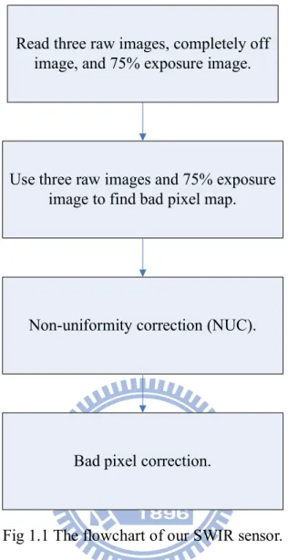
Our SWIR sensor has to be fast, easy to use, and lightweight. Consequently, the two-point correction method is simple and thus will be useful. In bad pixel correction, we will find some bad pixel maps. The Sobel edge is easy to use and fast. Because of bad pixels include non-responsive, dark pixels or always responsive pixels. The completely off image and 75% exposure image should be used. We will use images which are completely off image and 75% exposure image to find bad pixel map. Then, we can correct the bad pixels from bad pixel map. Our SWIR sensor flowchart is illustrated in Fig. 1.1 below.

Read three raw images, completely off image, and 75% exposure image.

Use three raw images and 75% exposure image to find bad pixel map.

Non-uniformity correction (NUC).

Bad pixel correction.

Fig 1.1 The flowchart of our SWIR sensor.

1.3 Color Edge Detection

In the review paper on color image segmentation, Ruzon and Tomasi [9] go further and group color edge detection methods into three classifications: output fusion methods, multidimensional gradient methods and vector methods. Output fusion methods apply single-channel edge detection techniques to each color plane and then combine the results.

In multidimensional gradient methods, the gradients from the individual channels are recombined before the edge decision, giving increase to a single edge calculation.

In [10], Scharcanski and Venetsanopoulos have proposed VOS-based approach. Trahanias and Venetsanopoulos used the reduced ordering (R-Ordering) by the VOS edge detectors of [5], [6]. The robust color morphological gradient (RCMG) edge detector [11] recognizes the maximum and minimum pixels in one process, however it does not discriminate between them. It is in contrast to the VOS edge detectors that sort the pixels in ascending order from the vector median to the vector extremum. The matrices are summed over all channels and the edge magnitude and direction given by the principal eigenvalue and the related eigenvector, respectively. Variations of this approach have been used by Cumani [12].

The difficult problem is how to combine the channels to give a final result that is with both output fusion and multidimensional gradient methods. For example, the simplest VOS operator is the vector range edge detector that measures the distance between the lowest and highest ranked vectors, i.e., the vector median and the vector extremum, respectively. The minimum vector dispersion (MVD) was proposed are shown to be the most effective in increasing the robustness to noise. However, the MVD is unable to provide an estimate of edge direction.

1.4 Automatic Thresholding Technique

Thresholding is a fundamental technique applied in many image processing applications. In robust machine vision systems, it would be important to automate the edge thresholding process which is adaptive to different image contents without manual interposition.

There are many thresholding algorithms published in the literature. The Otsu [13] algorithm is based on discriminant analysis and uses the zeroth-order and the

first-order cumulative moments of the histogram for calculating the value of the thresholding level. The Rosin algorithm [14] fits a straight line from the peak of the intensity histogram to the last non-empty bin. The point of maximum deviation between the line and the histogram curve will usually be located at a corner which is selected as the threshold value. The new feature image proposed by Rakesh [15] makes it easier to determine hysteresis thresholds.

It is a difficult assignment to selecting an appropriate thresholding. The problem is that different algorithms typically produce different results since they make different assumptions about the image content. Therefore, we will introduce an automatic thresholding method that can find the best hysteresis thresholds from all possible parameters.

1.5 Thesis Outline

The thesis is organized as follows. The basic concepts and technique concerning the NUC and bad pixel correction introduced in Chapter 2. In Chapter 3, the results of our SWIR sensor which is introduced in Chapter 2 are shown and compared. In Chapter 4, we describe our edge detection and automatic thresholding method and compared the experiment results of our automatic color edge detection techniques. At last, we conclude this thesis with a discussion in Chapter 5.

Chapter 2 The Improvement of NUC and Bad

Pixel Correction

2.1 NUC

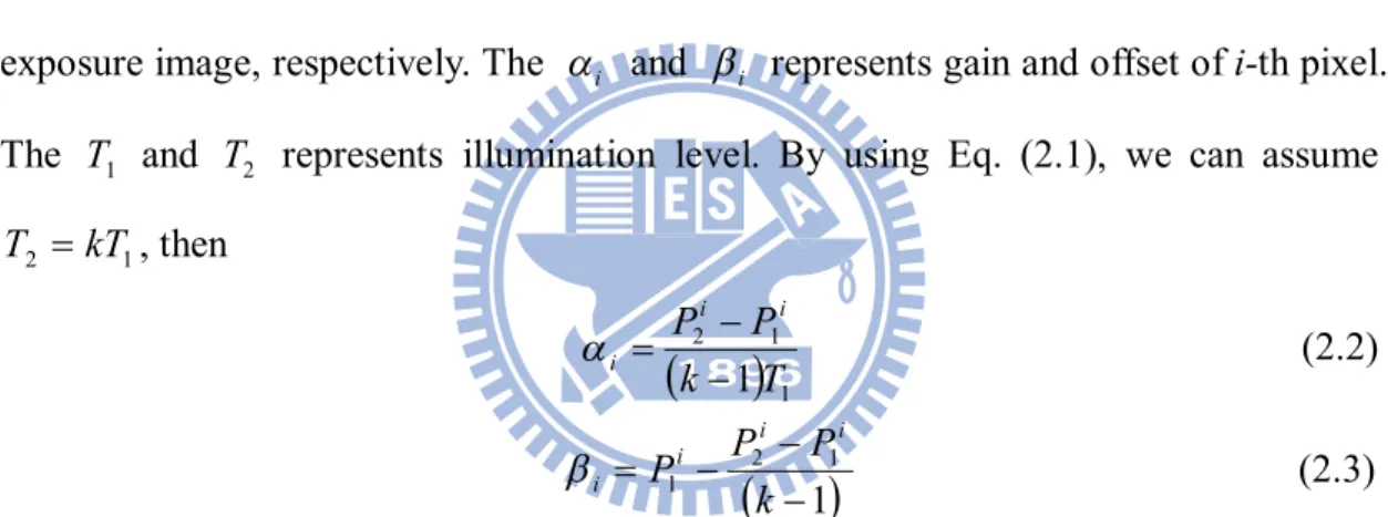
To implement two-point correction method for image sensor, we can assume          i i i i i i T P T P     1 1 2 2 , (2.1) where P₁i and P₂i represents the i-th pixel value in completely off image and 75% exposure image, respectively. The  and _i  represents gain and offset of i-th pixel. _i

The T and ₁ T represents illumination level. By using Eq. (2.1), we can assume ₂

1 2 kT T  , then





1 1 2 1 T k P Pi i i     (2.2)



1



1 2 1     k P P P i i i i  (2.3) Calculate averages that completely off image and 75% exposure image which are shown in Figs. 2.1(a)(b) as P and ₁ P , respectively. ₂

(a) (b)

Assuming under T and ₁ T , all pixels output should be the same level. In other ₂

word, P and ₁ P after correction ₂

         i i i i i i i i B T A P B T A P     1 1 2 2 (2.4) By using Eq. (2.2), and Eq. (2.3), then













i i i i P P P P T T P P A 1 2 1 2 1 2 1 2        (2.5)



1 1



1 T A P B _{i i} i i     (2.6) We want to correct infrared image which is under unknown illumination level T , _x

then i i x i i x T P   (2.7) Consequently, corrected pixel output signal should be



_i





_i



i i x i i i x i i i c P P P P P P P B T A P 1 2 1 2 1 1         (2.8) Therefore, it can correct directly without any other illumination level that have to using laboratory for reference.

2.2 Bad Pixel Correction

In bad pixel correction, Sobel edge detection is very important which is fast and easy. The masks show in Fig. 2.2, called the Sobel operators.

(a) x-direction. (b) y-direction. Fig. 2.2 The Sobel operators.

The difference between the third and first columns of the 3 3 image region approximates the derivative in the x-direction as shown in Fig. 2.2(a); and the difference between the third and first rows approximates the derivative in the

y-direction as shown in Fig. 2.2(b). The idea behind using a weight value of 2 is to

achieve some smoothing by giving more importance to the center point. Note that the coefficients in all the masks shown in Fig. 2.1 sum to 0, indicating that they would give a response of 0 in an area of constant gray level, as expected of a derivative operator.

First, we want to detect bad pixel map by using Sobel edge detection. Consider a grayscale image I with size m  be represented by vector n I ,

 

i j . By using SWIR sensor, we capture three different images. Therefore, three grayscale imagesI₁

 

i,j ,

 

i j

I₂ , , andI₃

 

i, j with size m  is shown in Figs. 2.3(a)n (c) which is called raw images, which is non-uniform correction is not activated.

(a)

(b)

(c)

Fig. 2.3 (a) The “Monitor” image. (b) The “Words” image. (c) The “Two-persons” image.

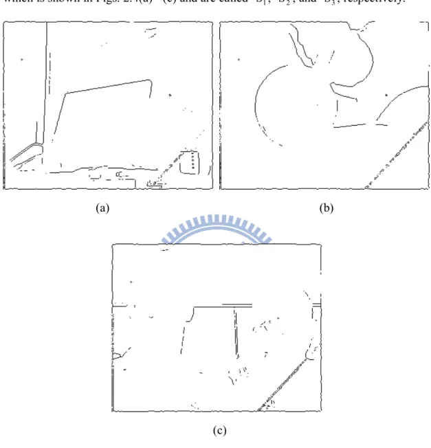
To obtain bad pixels of the image sensor, we first apply Sobel edge operation on these three images. After the operation, we have obtained three edge map images, which is shown in Figs. 2.4(a)(c) and are called S , ₁ S , and ₂ S , respectively. ₃

(a) (b)

(c)

Fig. 2.4 By Sobel edge detection, (a) “Monitor” image, (b) “Words” image, and (c) “Two-persons” image.

Then, we calculate four-directional difference d ,



i j



in the 3 3 window as shown in Fig. 2.5. The value d ,



i j



can be calculated by





i, j  I

 

i, j I



i1, j



 I

 

i, j I



i, j1



 I

 

i, j I



i1, j



 I

 

i, j I



i, j1



d ,

(2.9)

where  represents an absolute value operator and



i,j



represents the i-th row and

j-th column in the grayscale image I.

-1

-1

-1

-1

4

0

0

0

0

Fig. 2.5 Four-directional neighborhood operator.

After calculating d ,



i j



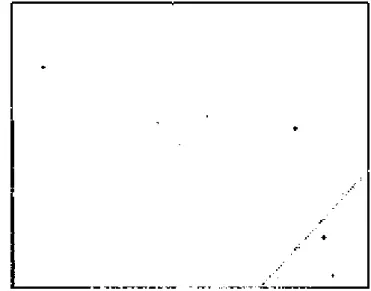
, we will select a threshold to pick up possible bad pixel candidates. For the 75% exposure image which is shown in Fig. 2.1 (a), we will find bad pixels possibility by using Eq. (2.9) and thresholding, with threshold value40, which is shown in Fig. 2.6. And it called d image. ₄

Finally, we calculate the fuzzy derivative donated as S_bp

 

i, j in each pixel

 

i,j . This is realized by the following fuzzy rule 1:

Fuzzy Rules 1.

IF S₁

 

i,j is an edge AND S₂

 

i,j is an edge AND S₃

 

i, j is an edge

OR S₁

 

i,j is an edge AND S₂

 

i,j is not an edge AND S₃

 

i, j is an edge

OR S₁

 

i,j is an edge AND S₂

 

i,j is an edge AND S₃

 

i, j is not an edge

OR S₁

 

i,j is not an edge AND S₂

 

i,j is an edge AND S₃

 

i, j is an edge THEN S_bp

 

i, j is an edge.

The AND operator (OR operator) can bethe minimum (maximum) that are the well-known triangular norms (together with their dual co-norms) in the fuzzy logic. For the not operator, we use the standard negator N

 

x  1x with x[0,1]. The

edge is the fuzzy set that was defined the point which is detected by Sobel edge

detection. According to fuzzy rule 1, we have S_bp edge map is shown in Fig. 2.7.

Fig. 2.7 The resulting image of at least two out of three images which is three Sobel edge map images.

Therefore, we use a rule for each edge point. We have two images which are Fig. 2.6 and Fig. 2.7 can estimate BP_map bad pixel map following rule 2.

Fuzzy Rules 2.

IF d₄

 

i,j is an edge OR S_bp

 

i, j is an edge. THEN BP_map

 

i, j is an edge.

The OR operator is the maximum in the fuzzy logic. The BP_map is shown in Fig. 2.8.

Fig. 2.8 The bad pixel map by using fuzzy rule 2.

Consequently, we can use the bad pixel map which is shown in Fig. 2.8 to do bad pixels correction with median filters shown in Chapter 3.

Chapter 3 Results of NUC and Bad Pixel

Correction

3.1 Results of NUC

First, we calculate standard deviation (STD) which is calculated by





,

1

1

2 1 1 2



















_

 n i i

x

x

n

s

_(3.1) where n is pixels number and x is







n i i

x

n

x

1

1

(3.2) We will use STD to estimate the performance of the NUC results. Therefore, we use Fig. 2.1(b) as a sample and its STD is 0.1349. It is to be noted that detected bad pixels shown in Fig. 2.8 are not included in calculating STD. By using Eq. (2.8), the result is shown in Fig. 3.1.

The STD of Fig. 3.1 becomes 0, in which bad pixels are not included in calculating STD. This great STD reduction after NUC shows its effectiveness in reducing the non-uniformity response among the pixels of image sensors. Applying NUC to “Monitor,” “Words,” and “Two-persons” images of Figs. 2.3(a)(c), the corrected images are shown in Figs. 3.2(a)(c), respectively.

(a) (b)

(c)

Fig. 3.2 The resulting images after NUC. (a) “Monitor” image, (b) “Words” image, and (c) “Two-persons” image.

To further validate the effectiveness of NUC, we exploit Sobel edge detection with a sensitive threshold to test raw images and NUC corrected images above,

leading to Figs. 3.3(a)(f), respectively.

(a) (b)

(c) (d)

(e) (f)

Fig. 3.3 Sobel edge map images of (a) “Monitor” raw image, (b) “Monitor” image after NUC, (c) “Words” raw image, (d) “Words” image after NUC, (e) “Two-persons” raw image, and (f) “Two-persons” image after NUC.

From these figures in Fig. 3.3, it is easy to see the powerfulness of NUC in reducing the excessive or un-necessary edges due to the non-uniformity of the image sensors. Excessive lines in left-up corner of Fig. 3.3(a) is removed in Fig. 3.3(b), NUC corrected counterpart. From Fig. 3.3(d), it is evident that removed of excessive lines and edges, in tables, wafer, and hand right, of Fig. 3.3(c). Unnecessary lines and edges of left person in Fig. 3.3(e) has been removed in NUC corrected image Fig. 3.3(f).

3.2 Results of Bad Pixel Correction

For the detected bad pixel map as shown in Fig. 2.8, we can use median filters to correct bad pixels. First, you can see in Fig. 2.8 that four boundaries are prone to bad pixels. If a boundary line is almost bad pixels, we employ neighborhood good row or column to replace it. After a boundary line with bad pixel rate exceeding 25% has to be replaced line wise. With this criterion (in effect), the three NUC corrected images are boundary replaced and are shown in Fig. 3.4. Comparison results are as follows in Fig. 3.4.

(a) (b)

(c) (d)

(e) (f)

Fig. 3.4 (a) “Monitor” raw image. (b) Four boundaries replaced of “Monitor” image after NUC. (c) “Words” raw image. (d) Four boundaries replaced of “Words” image after NUC. (e) “Two-persons” raw image. (f) Four boundaries replaced of “Two-persons” image after NUC.

Correcting four boundaries bad pixels, the bad pixel map will be updated as shown in Fig. 3.5.

Fig. 3.5 The bad pixel map after correcting four boundaries bad pixels.

Second, we use a 5 5 median filter to correct bad pixels and the results are shown in Figs. 3.6(a)(c).

(a)

(b)

(c)

Fig. 3.6 The resulting of 5 5 median filter corrected (a) “Monitor” image. (b) “Words” image. (c) “Two-persons” image.

In Figs. 3.6(a)(c), it can be easily seen that these still are bad pixels on the lower right corner of images. Consequently, we only use Eq. (2.9), four-directional neighborhood operator with threshold value150, to calculate the bad pixel map again. The bad pixel maps are shown in Figs. 3.7(a)(c).

(a) (b)

(c)

Fig. 3.7 The resulting images after four-directional neighborhood operator, on Fig. 3.6 (a) “Monitor” image, (b) “Words” image, and (c) “Two-persons” image.

In the sequel, we use a 3 3 median filter on Fig. 3.6 to correct bad pixels of Fig. 3.7 again. The resulting images are shown in Figs. 3.8(a)(c).

(a)

(b)

(c)

Fig. 3.8 The resulting images of 3 3 median filter corrected images of Fig. 3.6 (a) “Monitor” image, (b) “Words” image, and (c) “Two-persons” image.

Notice that the median filter is useful on bad pixels correction. Moreover, median filter is computational easy and is appropriate for a real-time ROIC implementation. We have also applied bad pixel correction with 3 3 median filter repeatedly for three times, whose results are similar to those obtained by 5 5

median filter and the 3 3 median filter. But it is need three times correction, and it is waste time. Therefore, we try to use 5 5 median filter once and then 3 3

median filter again. The results are good and efficient. Finally, we choose 5 5

median filter once and the3 3 median filter again. For comparison, the raw images and the corrected images are shown in Figs. 3.9(a)(f).

(a) (b)

(c) (d)

(e) (f)

Fig. 3.9 (a) “Monitor” row image. (b) The resulting image of NUC and bad pixel corrected image of “Monitor.” (c) “Words” row image. (d) The resulting image of NUC and bad pixel corrected image of “Words.” (e) “Two-persons” row

image. (f) The resulting image of NUC and bad pixel corrected image of “Two-persons.”

The difference between the row images and the corrected images are tremendous. We adjust the non-uniformity among image sensor pixels and correct bad pixels by using fast and efficient algorithm. The processed images have been greatly improved by our proposed efficient scheme.

Chapter 4 Edge Detection Techniques for Bad

Pixel Detection

Edge detection plays an important role in bad pixel detection of optical sensor chip. In image processing, edge detection is also very useful on tasks such as segmentation, pattern recognition, object tracking, and image coding. The performance of these problems is greatly affected by good edge detection. We use Sobel edge detection and four-directional neighborhood operator to detect bad pixels and test NUC in Chapters 2 and 3. These techniques are basic edge detection methods. In Sobel edge detection and four-directional neighborhood operator, we calculate each pixel’s edge level and select a threshold manually. However, the best edge detection will use an automatic threshold technique to select the best threshold.

Edges will not be detected in grayscale images when neighboring objects have different hues but equal intensities since the color cue is lost during grayscale conversion. Such objects cannot be distinguished in grayscale images. Similar gray tone objects are treated as one big object in the scene. Additionally, edge detection is sometimes difficult in low contrast images but rather sufficient results can be obtained in color images. To obtain more meaningful edges, there has been an increased interest in color edge detection. Humans can differentiate thousands of colors compared to about 256 shades of gray; hence, grayscale images do not carry all the edge information that human visual system (HVS) can detect. In this chapter, we propose an improvement of color edge detector based on vector order statistics. We use the concept of fuzzy gradient to calculate the direction of the gradient for every pixel in the image. For using an adjustable window according to the direction of the gradient, it is more accurate to calculate the local maximum edge response for every

pixel, and an automatic threshold technique is adaptive to threshold the local maximum edge response for the image content.

4.1 Vector Order Statistics

4.1.1 Vector Order Statistics Review

Scalar order statistics have played an important role in the design of robust signal analysis techniques. This is due to the fact that any outliers will be located in the extreme ranks in the sorted data. Consequently, these outliers can be isolated and filtered out before the signal is further processed. Ordering of univariate data is well defined and has been extensively studied in order statistics [16]. Let the n random

variables X , _i i = 1, 2, …, n , be arranged in ascending order of magnitude as

X₍₁₎  X₍₂₎  ...  X_{( )n} (4.1) Then the i-th random variable X_{( )i} is the so-called ith order statistic. The minimum X₍₁₎, the maximum X_{( )n} , and the median X_(n2) are among the most important order statistics, resulting the min, the max, and the median filters, respectively.

The concepts are, however, not straightforwardly expanded to multivariate data since there is not any universal way of defining an ordering in multivariate data. There has been a number of ways proposed to perform multivariate data ordering that are generally classified into the ordering of multivariate data [17]: marginal ordering (M-ordering), reduced or aggregate ordering (R-ordering), partial ordering (P-ordering), and conditional ordering (C-ordering).

4.1.2 Characteristics of Vector Order Statistics

Let X represent a p-dimensional multivariate X [X X₁, ₂,...,X_p]T where ,

l

X l 1, 2, …, p are random variables and let X i, i 1, 2, …, n be an

observation of X. Each X is a i p-dimensional vector Xi [X X₁i, ₂i,...,Xi_p] .T In M-ordering, the multivariate samples are ordered along each one of the -dimensions

p independently. For color signals, this is equivalent to the separable method where each one of the colors is processed independently. The i-th marginal order statistic is the vector X( )i  [X₁( )i ,X₂( )i ,...,X_p( )i ] ,T where X_r( )i is the ith

largest element in the r-th channel. The marginal order statistic X( )i may not correspond to any of the original samples X X1, 2,...,X as it does in one dimension. n

In R-ordering, each multivariate observation X is reduced to a scalar value i d _i

according to a distance criterion. A metric that is often used is the generalized distance to some point. The samples are often arranged in ascending order of magnitude of the associated metric value d _i.

In P-ordering, the objective is to partition the data into groups or sets of samples, such that the groups can be distinguished with respect to order, rank, or extremeness. This type of ordering can be accomplished by using the notion of convex hulls. However, the determination of the convex hull is difficult to do in more than two dimensions. Other ways to achieve P-ordering are special partitioning procedures and thus are not preferred. Another drawback associated with P-ordering is that there is no ordering within the groups and thus it is not easily expressed in analytical terms. These properties make P-ordering infeasible for implementation in digital image processing.

In C-ordering, the multivariate samples are ordered conditionally on one of the marginal sets of observations. This has the disadvantage in digital image processing that only the information in one component (channel) is used.

From the above, it is evident that R-ordering is more appropriate for color image processing than the other vector ordering methods. If we employ as a distance metric the aggregate distance of X to the set of vectors i 1 2

, ,..., n X X X , then 1 , n i k i k d X X  

_

 i 1, 2, ..., n (4.2) where  represents an appropriate vector norm. The arrangement of the d s in _i

ascending order



d₍₁₎  d_{( 2)} ... d_{( )n}



, associates the same ordering to the multivariate X s. i

X(1)  X(2)  ... X( )n (4.3) In the ordered sequence, X(1) is the vector median of the data samples which is introduced by vector median filters [18]. It is defined as the vector contained in the given set whose distance to all other vectors is a minimum. Moreover, vectors appearing in low ranks in the ordered sequence are vectors centrally located in the population, whereas vectors appearing in high ranks are vectors that diverge mostly from the data population. These samples are generally called “outliers.” It follows that this ordering scheme gives a natural definition of the median of a population and of the outliers of a population.

4.2 VMD Detector

For a color image I of size m  , each pixel location n

 

i, j is represented by a three-tuple color vector I

 

i, j 



I₁

 

i, j, I₂

 

i, j , I₃

 

i, j



, in which I_p

 

i, j

denoting the p-th component of a color space for i1,2,...,m and j1,2,...,n. For each pixel location

 

i, j , by using a 33 window, we compute the local sum of distances to describe the relationship between the current pixel vector I ,

 

i j and its neighboring pixel vectors. Let d_l

 

i, j be the local sum of distances for the current pixel vectorI ,

 

i j , then

 

_{ }



 





       1 1 1 1 , , , i i k j j h l i j I i j I k h d

(4.4)

where  represents a 2-norm. After we have computed the local sum of distances

 

i j

d_l , of the current pixel location

 

i,j , we sort the distance values in the neighboring area in ascending order d_l(1)  d_l(2) ...  d_l(9). The distance values

(1)

l

d and d_l(9) correspond to the minimum and the maximum of the nine distance values, respectively.

By the concept of R-ordering, the ordering of d_l(1)  d_l(2)  ...  d_l(9)

associates the same ordering to the pixel vectors, X(1)  X(2)  ... X(9),which means that X(1) is the pixel vector having the smallest local sum of distances and

(9)

X is the pixel vector having the largest local sum of distances. Therefore, if the current pixel location

 

i,j has an edge, the vector I ,

 

i j must have a larger response of d_l

 

i, j .

Although we now obtain the information on the smallest and the largest local sum of distances, the information contained among vectors X(1), X(2), ..., X(9)

should also be captured and be useful for edge detection. The maximal variation among vectors is an indication of the distribution of the nine vectors. Since that vectors X(1), X(2), ..., X(9) correspond to the ordering of the aggregate distances, the confined maximal variation MV among these vectors can be simply defined as _c

MV_c max



X i Xi1



, i 1, 2, ..., 8 (4.5) When the value MV is determined, we can also determine the exact two _c vectors X( )i and X(i1) which correspond to MV . _c X( )i and X(i1) further suggest that X(1), X(2), ..., X(9) can be classified into two clusters: (1) vectors,

(1) ( 2) ( )

, , ..., i ,

X X X from smaller side of the edge, and (2) vectors,

( 1) ( 2) (9)

, , ..., ,

i i

X  X  X from larger side of the edge. Let M and _s M be the mean _l

vector of the vectors X(1), X( 2), ..., X( )i , and the vectors X(i1), X(i2), ..., X(9)

respectively. Thus, VMD can be defined as

VMD  M_l  M_s (4.6) VMD detect the variation between two sides of edge (larger and smaller side) by a distance measure. Consequently, in a uniform area, where all vector values are close to each other, the output of VMD will be small. On the other hand, the output of VMD will be large since M and _s M are the mean vectors of two sides of the edge. _l

The VMD method suffers from the disadvantage of the weak ability for detecting oblique edges due to the fact that its gradient magnitude is derived from the fixed window with the distance between the mean vector of the large side and the mean vector of the small side. In addition, in the presence of noise and for non-ideal edges, the maximal variation that splits the window into the large side and small side may not represent the distribution among the vectors in the fixed window, and then the

VMD may produce an edge response that is not necessarily representative of the real gradient.

To avoid these problems, we use an adjustable window that can rotate its orientation according to the direction of the gradient. In the 3 3 window, we classify the direction of the gradient to four orientations, i.e., WE direction (0 ), 

SWNE direction (45 ), S N direction (90 ), and SE NW direction (135 ) that can  be determined by the fuzzy gradient value which is introduced by the fuzzy image filter [7] and the fuzzy random impulse noise reduction method (FRINR) [8]. Thus, the new proposed method will combine VMD with the fuzzy image filter and FRINR that have the ability to estimate the direction of the gradient for each pixel and adjust the window for more exactly detecting edge response.

In our approach, there are two steps that are used to define the direction of the gradient for each pixel in the color image. First, consider a color image I with size

n

m  be represented by color vector I

 

i, j 



I₁

 

i, j, I₂

 

i, j , I₃

 

i, j



, in which

 

i j

I_p , denoting the p-th component of a color space, we calculate g ,



i j



and





i j mg , in the 3 3 window as

 





 

8 , , , 1 1 1 1

 

       k h j i I h j k i I j i g (4.7)

 





 

8 , , , 1 1 1 1

 

       k h j i g h j k i g j i mg (4.8) where  represents a 2-norm and



i,j



represents the i-th row and j-th column in the color image I. Because edge pixels and corrupted impulse noise pixels generally cause large g ,



i j



value, we also calculate mg ,



i j



that can help us to distinguish edge pixels and noise pixels. To discriminate edge pixels and noise pixels, we can define a fuzzy set denoted as large, and it corresponds to the membership function

which is shown in Fig. 4.1. We see that we have to determine two important parameters a and b. The parameters a and b can be defined as

a

 

i,j mg



i,j



(4.9) b

 

i,j a



i,j



0.2a

 

i,j (4.10)

Fig. 4.1 The membership function corresponds to large.

Second, we consider a 3 3 neighborhood around the central pixel I ,



i j



. Each of the eight neighbors of I ,



i j



corresponds to one direction {North West (NW), North (N), North East (NE), East (E), South East (SE), South (S), South West (SW), West (W)} that is displayed in Fig. 4.2(a). We use the concept of the fuzzy gradient value which contains the basic gradient value and the related gradient value. The basic gradient value is donated as _DI



i,j



of pixel position



i,j



in direction

For example, _NWI

 

i, j I



i1, j1



I

 

i, j (4.11) _NI

 

i, j I



i, j1



I

 

i, j (4.12)

N

S

E

W

(i,j)

NW

NE

SW

SE

(a) (b)

Fig. 4.2 (a) The neighborhood around the central pixel I ,



i j



. (b) Pixel indicated in gray are used to compute the fuzzy gradient value of pixel I ,



i j



TABLE 4.1

The fuzzy gradient in each direction

D Basic gradient Related gradient Correspond direction

NW N NE W E SW S SE





i j I NW , 





i j I N , 





i j I NE , 





i j I W , 





i j I E , 





i j I SW , 





i j I S , 





i j I SE , 





1, 1 _NWI i j , _NWI



i1, j1







, 1 _NI i j , _NI



i, j 1







1, 1 _NEI i j , _NEI



i1, j1







i j I W 1,  , _WI



i1, j







i j I E 1,  , _EI



i1, j







1, 1 _SWI i j , _SWI



i1, j1







, 1 _SI i j , _SI



i, j 1







1, 1 _SEI i j , _SEI



i1, j1



SWNE (45 )  WE (0 )  SENW (135 )  SN (90 )  SN (90 )  SENW (135 )  WE (0 )  SWNE (45 ) 

Next, we also calculate the related gradient value which corresponds to each of eight directions. For example, Fig. 4.2(b) shows the related gradient of the NW direction and it can be expressed as

NWI

 

i,j NWI



i1, j1



I



i,j2



I



i1,j1



(4.13)



,







1, 1







2,







1, 1



 _NWI i j _NWI i j I i j I i j (4.14) In Table 4.1, we show a detail of the eight directions in the column 1, the basic gradient corresponds to each direction in column 2, the two related gradients correspond to each direction in column 3, and the correspond perpendicular direction in column 4. Actually, in the3 3 window, the direction of the gradient only belong to WE direction (0 ), SW NE direction (45 ), S N direction (90 ), and SE NW

direction (135 ). Thus, we can only compute the fuzzy gradient for the direction set 

ED where ED



NW,N,NE,W



that contains all the orientations in the 3 3

window. For example, computing the fuzzy gradient for the NW direction and SE direction are both equivalent to computing the gradient for the SWNE direction

(45 ). 

For each direction of the direction set ED, we calculate the fuzzy derivative donated as P

 

i, j in each pixel

 

i, j for direction P, whereP ED. This is

realized by the following fuzzy rule 3.

Fuzzy Rules 3.

IF _PI

 

i, j is large AND _PI



i, j



is large AND  _PI



i, j



is large

OR _PI

 

i, j is large AND _PI



i, j



is not large AND  _PI



i, j



is large

OR _PI

 

i, j is large AND _PI



i, j



is large AND  _PI



i, j



is not large THEN P

 

i, j is large in direction P.

The AND operator (OR operator) can bethe minimum (maximum) that are the well-known triangular norms (together with their dual co-norms) in the fuzzy logic. For the not operator, we use the standard negator N

 

x  1x with x[0,1]. The

large is the fuzzy set corresponds the membership function LARGE that was defined

above. The idea of this rule is to consider an edge passing though the pixel I ,



i j



and its neighborhood for the direction, i.e. SW-NE direction (45 ), not only the basic  gradient value _PI

 

i, j will be large, but also the related gradient _PI



i, j



or



i j



I

P ,

  can expect to be large.Therefore, if two out of three gradient values are small, it is safe to assume that no edge exists in the considered direction.

Fig. 4.3 The membership function corresponds to absolute value.

Next, we again use a rule for each direction. The idea behind the rule is that if a pixel is assumed to be large in rule 3, then it probably can be consider as an edge for direction P, and the derivative value will be used to estimate the gradient direction of this pixel. Thus, we use the following rule 4 to computeD_gradientP .

Fuzzy Rules 4.

IF P

 

i, j is large AND PI

 

i,j is absolute value

THEN D_gradientP is absolute value in direction P.

Where the fuzzy set absolute value corresponds to the membership function which is shown in Fig. 4.3 and the parameter L255 is used in the experiment. The AND operator is also the minimum in the fuzzy logic.

The final step in the computation of the fuzzy gradient is the defuzzification. We are interested in obtaining the direction that has maximum value ofD_gradientP . P , *

which is estimated to be the gradient direction in pixel

 

i,j , is determined by P D_gradientP I

 

i j ED P , max arg    (4.15) Finally, we rotate the window with the angle that corresponds to P . For using *

the adjustable window, the VMD method will be more robust for detecting the edge response. The experiment will be discussed in Chapter 4.4.

4.3 Automatic Threshold Selection

To automatically obtain the best threshold that is adaptive to the image contents, we propose a new method for hysteresis thresholding method combining the merits of Yitzhaky and Peli [19] and Medina et al. [20] methods. Yitzhaky and Peli can find the best thresholds within a set of possible values, but the performance will depend on the set of possible values chosen. On the other hand Medina et al. method is similar to Yitzhaky and Peli, but the performance will depend on one’s choice of the subset and the overset. In the following, we will introduce how to apply the thresholding methods to VMD method.

4.3.1 Determine Parameter Set

Fig. 4.4 shows the symbolic graphic of the choice of parameter set. For an image I,

let E_I be the unknown true edge points set of the image I with the condition

I I

I E B

A   where A_I and B_I are the subset and the overset of the image I. For a possible hysteresis thresholdsset C, for example



tlow thigh tlow thigh tlow thigh



C ( , ) , [0, 1], 

we want to find the parameter set T in the region between the subset A_I and the overset B_I. Thus, we will get the best edge map

high

lowt

t

E _, determined by hysteresis thresholds t_low and t_high with (t_low,t_high)T in the next section.

Fig. 4.4 The symbolic graphic of the choice of parameter set [20].

Considering the feature image histogram is usually unimodal, we use the Otsu method [13] and the Rosin method [14] to determine the subset A_I and the overset

I

B . The Otsu method is not very sensitive on unimodal histograms and performs rigorously on detecting edge points for edge detection, but edge pixels detected by the Otsu method have a high probability of being true edge points. Thus, the edge map

Otsu

E can be utilized as the subset of the image. The Rosin method is very sensitive on unimodal histograms and it can be noisy for edge detection, but the Rosin method can usually detect the true edge pixels together with many fakery ones. Thus, the edge map E_Rosin can be employed as the overset of the image. If the conditions

sin ,t Ro

t E

E

high

low  and EOstu Etlow,thighhold, then the following expression can easily

be proved 0 ) , (E_{t ,t} E_Rosin  FP high low FN(E_{t ,t} ,E_Ostu)0 high low (4.16)

where FP and FN are False Positive and False Negative in ROC analysis [21]. Here,

FP indicates that the points were decided as edges in

high

lowt

t