基於等位函數法之運動物體偵測與追蹤

國

立

交

通

大

學

電子工程學系電子研究所碩士班

碩

士

論

文

基於等位函數法之運動物體偵測與追蹤

Detection and Tracking of Moving Objects based on

Level Set Theory

研 究 生： 蔡孟修

指導教授： 王聖智 博士

基於等位函數法之運動物體偵測與追蹤

Detection and Tracking of Moving Objects based on

Level Set Theory

研 究 生：蔡孟修 Student：Meng-Hsiu Tsai

指導教授：王聖智 博士 Advisor：Sheng-Jyh Wang

國 立 交 通 大 學

電子工程學系 電子研究所碩士班

碩 士 論 文

A Thesis

Submitted to Department of Electronics Engineering & Institute of Electronics College of Electrical Engineering and Computer Science

National Chiao Tung University in partial Fulfillment of the Requirements

for the Degree of Master in

Electronics Engineering June 2006

Hsinchu, Taiwan, Republic of China

基於等位函數法之運動物體偵測與追蹤

研究生：蔡孟修 指導教授：王聖智 博士

國 立 交 通 大 學

電子工程學系 電子研究所碩士班

中文摘要

監控系統中的單一攝影裝置通常包含建立背景模型、偵測運動物

體、追蹤運動物體等三個步驟。在本論文中，我們將討論如何在這些

步驟當中，運用等位函數法來記錄運動物體的輪廓。在整個運動偵測

與追蹤的過程中，我們首先建立環境模型以利於使用「背景相減法」

來達成運動物體偵測。當使用動態攝影機來追蹤運動物體時，由於背

景資訊會隨時間改變，此時需要改採「區塊追蹤模型」才能持續追蹤

運動物體。為了減低背景環境的干擾，原始的區塊追蹤模型會被加以

修改，以考慮前後兩張畫面等位函數曲面之間的交互關係。此外，利

用畫面中統計特性加入機率預測的模型，可增強區塊追蹤的強韌性。

論文最後會提出一套整合的監控系統架構，架構中的不同元件會選擇

採用適當的輪廓模型來分別解決運動物體偵測與追蹤的問題。

Detection and Tracking of Moving Objects based on

Level Set Theory

Student：Meng-Hsiu Tsai Advisor：Sheng-Jyh Wang

Department of Electronics Engineering, Institute of Electronics

National Chiao Tung University

Abstract

An intelligent video surveillance system usually performs the tasks of

background modeling, motion detection, and tracking. In this thesis, a

level set function is used to record the moving objects for these three

operations. The background model is first constructed before the

background subtraction is performed for the motion detection. Then, a

mobile camera keeps tracking the moving objects with a region tracking

model. The original region tracking model is modified to alleviate the

interference of cluttered environment. The relation between two level

surfaces of successive two frames is taken into consideration. The

probability model built from the statistic property of an image is also

included. Finally, an integrated surveillance system is proposed. Different

units in the surveillance system may choose appropriate contour models

to solve their problems.

誌 謝

感謝王聖智老師兩年多來的教導，老師豐富的學識與涵養讓我獲

益良多。感謝實驗室的所有同學，陪我度過這段大家共同學習的日

子。感謝與我一起加油打氣的朋友們，你們給我的鼓勵是讓我在挫折

中堅持到最後的原動力。感謝我的家人，我珍惜你們多年來對我的支

持與包容，我愛你們。

Contents

中文摘要……… i

Abstract ……...……….……... iii

誌 謝 ... v

Chapter 1. Introduction...1

Chapter 2. Active Contours ...5

2.1 Snake Model...5

2.2 Geodesic Active Contour...6

2.3 Level Set Theory ...11

2.4 Active Region Model ...15

Chapter 3. Detection and Tracking of Moving Objects...23

3.1 Motion Detection with Background ...23

3.1.1. Active Contours without Edges ...24

3.1.2. Background Subtraction ...30

3.2 Region Tracking ...33

3.2.1. Region Tracking without Motion Computation ...33

3.2.2. A New Region Tracking Model ...37

3.3 Probability Model...42

3.3.1. Kernel Density Estimation...43

3.3.2. ML and MAP Estimation ...45

Chapter 4. Implementation Issues and Experimental Results ...51

4.1 Implementation Issues ...51

4.1.1. Distance Transform...51

4.1.2. Solve PDE Numerically...55

4.1.3. Re-initialization ...58

4.2 Build Background...63

4.2.1. Motion Detection without Background...63

4.2.2. Background Modeling ...66

4.3 Experimental Results...68

Chapter 5. Conclusions...75

List of Figures

Figure 1-1 General framework of a visual surveillance system [20]. ...2

Figure 2-1 Snake Model...5

Figure 2-2 Level Surface and Contours ...12

Figure 2-3 Geodesic Active Contour initialized totally outside the objects...15

Figure 2-4 Geodesic Active Contour with bad initialization. ...15

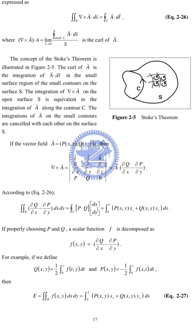
Figure 2-5 Stoke’s Theorem...17

Figure 2-6 Convergence of active contours with region information. ...20

Figure 2-7 Convergence of active contours with some objects are partly outside the image...20

Figure 2-8 Convergence of active contours when the initial curve is too small. ...21

Figure 3-1 Background Subtraction. (a) Background Image. (b) Frame 180. ...24

Figure 3-2 F₁(C) and F₂(C). Four situations of F₁(C)andF₂(C) with different contours. When the image data inside and outside the contours are not uniform, the values of F₁(C)orF₂(C)produce a positive value. Only when the contours matches the boundaries of the objects, bothF₁(C)andF₂(C)are zero and the energy function in (Eq. 3-1) reaches its minimum. ...25

Figure 3-3 Active contours without edges. c1 and c2 are the average values inside and outside the contours, respectively. ...26

Figure 3-4 Apply the “active contours without edges” method to the Gaussian smoothed image. c1 and c2 are the average values inside and outside the contours, respectively...27

Figure 3-5 Apply the “active contours without edges” approach to the image with Gaussian noise. The standard deviation of the noise is 30. ...27

Figure 3-6 Statistical histogram of Figure 3-5. The blue bar is the histogram of the whole image, the red bar is the histogram of the inside region, and the green bar is the histogram of the outside region. ...28

Figure 3-7 Apply the “active contours without edges” approach to the image with Gaussian noise. The standard deviation of the noise is 80...29

Figure 3-8 Apply the “active contours without edges” approach to the image with improper initialization. The standard deviation of the noise is 20. Note that c1 is larger than c2. The region “inside” the contours is actually the background region. ...29

“Hall” test sequence...31

Figure 3-10 Classify the difference image data of Frame 180 and Frame 1 of the

“Hall” test sequence. The initial contour is replaced by a few small contours...31

Figure 3-11 Apply the “active contours without edges” model to the hall sequences.

Frame 1 is taken as the background. Multiple objects are successfully identified based on the level set approach. ...32

Figure 3-12 Comparison of required time of two different initializations. The solid

line denotes the required time based on the large contour, while the dot line denotes the required time based on the set of small contours...32

Figure 3-13 The force F defined by the region tracking model. (a) The pre-defined

region in the reference frame. (b) The pixels where F <0 in the current frame...37

Figure 3-14 Apply the morphing operator to the level surface of the reference frame.

(a) The level surface of the reference frame. (b) Morphing result. (c) Apply a low-pass filtering and the re-initialization to the surface in (b). (c) is used to estimate the new level surface in the current frame. ...38

Figure 3-15 The region force with and without the weight P . The cracked false _ϕ

detected points are reduced by adding P . The influence of the _ϕ

surrounding environment is reduced and makes the region tracking model more robust. ...39

Figure 3-16 The car-phone test sequences. The face region is defined in the first

frame. The level surface is only updated inside the green rectangle. The face is successfully tracked even though the scene changes outside the car...40

Figure 3-17 Football sequences. The camera moves very quickly and the target is

blurred in some frames. The contour does not grow incorrectly due to the use of n (x)

estimate v

ϕ in (Eq. 3-17)...40

Figure 3-18 Football sequences with original region tracking model. The contour

grows incorrectly because of the interference of the environment clutter. ...41

Figure 3-19 Track a small target in the coastguard sequence. The level surface with

higher resolution is only evaluated inside the green rectangle. More computational resources can be allotted to a specific region and produce a higher quality result...41

Figure 3-20 Use a level surface with lower resolution. This reduces large

computational cost. The essential position is successfully tracked but the fine boundary of the object is lost...42

Figure 3-21 The blue line is the histogram of the gray-level Lena image. The red

line is the kernel density estimation result...44

Figure 3-22 Improper kernel bandwidth selection. If the bandwidth is too small, it

causes under-smoothed. If the bandwidth is too large, it causes over-smoothed...44

Figure 3-23 Maximum likelihood. (a) The preset contours which define the objects in

the reference frame. (b) The objects move in the current frame. (c) The probability of inside region in the current frame. (d) The probability of outside region in the current frame. (e) and (f) are the histograms inside and outside the contours in (a). ...45

Figure 3-24 Maximum likelihood estimation. (a) Define the object in the reference

frame. (b) The current frame. (c) The probability of the inside region according to the distribution in the RGB space. The RGB space is divided into 16×16×16 bins. ...46

Figure 3-25 Obtain the prior information. The current frame is divided into many

blocks. Every block finds the most matched region within a search range in the reference frame. Then the proportion of R0 is used to

estimate the priorP(IN) for all pixels of Block( i , j ) in the current frame. ...48

Figure 3-26 The probability characteristic of the current frame in Figure 3-24 (b). (a)

and (b) are the color version of Figure 3-23 (c) and (d). (c) is the prior information obtained by (Eq. 3-22). (d) is the MAP estimation from (Eq. 3-21). ...49

Figure 3-27 Merge the inside information of the new region tracking model and the

probability model. The total inside information can be formed by using different amounts of weight for the two components. ...49

Figure 3-28 The experimental result of real sequences acquired in the laboratory.

The contour of the person is preset in the first frame. ...50

Figure 4-1 Distance Transform. In (b), the values outside the object depend on their

distance away from the object...52

Figure 4-2 Two-pass algorithm in 2D. The binary input image is shown as the right

star image. The first pass accumulates the distance value from top-left to bottom-right, while the second pass accumulates the distance value from bottom-right to top-left...53

Figure 4-4 Error propagation result due to improper approximation of∇ ...55 ϕ Figure 4-5 The propagation of the 1-D level set function. The solid blue line is the

level set function and the green line is the value of the velocity function. ...57

Figure 4-6 Re-initialization demonstration of (Eq. 4-8). The green line is the preset

level function and the blue line shows the variation of the level function according to the re-initialization procedure. The time step is set to be 0.5. ...59

Figure 4-7 The propagation of the level set function with velocity F in Figure 4-5

and adopt the re-initialization at the end of each time step. The glitches in Figure 4-5 are eliminated...60

Figure 4-8 The re-initialization in two dimension space. The level function is

initially set to be -1 inside the objects and 1 outside the objects. ...62

Figure 4-9 Motion Detection by thresholding the inter-frame difference image. The

black pixels represents the motion block with the measurement d...64

Figure 4-10 Make a solid detection result. (a) The blue blocks show the original

SAD detection result. (b) Morphological closing with a 3x3 structuring element. (c) Morphological closing with a 5x5 structuring element. (d) Fill the hole inside the moving object via (Eq. 4-11)...65

Figure 4-11 Contour propagation using (Eq. 4-11). ...66 Figure 4-12 Test sequences for background modeling. ...67 Figure 4-13 Background modeling process with n = 30. The white regions are the

background region. ...67

Figure 4-14 Background modeling using different n’s. (a) n = 30, (b) n = 60. The

discontinuous regions in the pink ellipses are due to the different intensity values from different frames. ...68

Figure 4-15 A simplified version of Figure 1-1. Every camera contains “background

modeling”, “background subtraction” and “region tracking” processes. ...69

Figure 4-16 Flow chart of a single camera’s system. This figure shows the details

about how to control the process of every camera in Figure 4-15...70

Figure 4-17 The simulation result of Figure 4-16. The images with green grid and

blue mask are in the background modeling status. When the background is modeled in all blocks, a background subtraction result is obtained. The frames with a green rectangle represent the tracking results. ...74

Figure 4-18 The consuming time of processing the sequence in Figure 4-17. The

modeling or background subtraction. The frames with a relatively large time consuming are in the status of region tracking. ...74

Chapter 1. Introduction

The applications of visual surveillance systems are getting more and more popular. Image capture devices become more available today. Moreover, powerful computers make complex digital image process more realizable. To make the image acquisition process more valuable, visual surveillance systems become smarter than before. Here, the analysis of moving objects could be the first important step. Some associated topics will be introduced and a brief introduction of this thesis will be given at the end of this chapter.

The visual surveillance system proposed in [20] is shown as Figure 1-1. A complete surveillance system may contain multiple cameras. These cameras cooperate with each other and the acquired information is fused. The tasks after the video acquisition step can be divided into two parts. One is motion detection and the other one is motion tracking.

In Figure 1-1, the detection part contains “environment modeling”, “motion segmentation”, and “object classification”. The environment or the background should be modeled before the moving objects can be recognized. Ahmed Elgammal et

al [18] proposed a way to model the foreground and background by using

nonparametric kernel density functions. In [19], a graph method like a finite state machine records the status of each pixel. The motion region is stored in a layer map. In [21], salient motion is detected without background information. This approach can resolve problems caused by luminance variation and slight movement of the background. (ex. wavering trees in an outdoor scene).

Figure 1-1 General framework of a visual surveillance system [20].

Regarding tracking, there exist many different methods for the tracking of objects in image sequences. Mean-shift [17] is a robust method to track an ellipse or rectangle region. Even though the size of the tracking window may change adaptively, this method doesn’t extract the boundary of moving objects. On the other hand, the snake model [1] proposed by Kass builds an energy function to control contour propagation. The contour finally locates at the boundary of an object to reach a local minimum of the energy function. Micheal Isard and Andrew Blake use B-spline curves to parameterize the contour for their CONDENSATION algorithm [22]. To further improve the performance of the snake model, Nikos Paragios et al [23] use the Geodesic Active Contours model to detect and track moving objects. The contours are described by a level surface. The level-set theory constructs the relation between the contours and the level surface. This level surface is very useful in the recording of multiple objects. In [25], the residuals of several frames after motion compensation

contour tracking for sequences acquired by a mobile camera.

Level set theory is a very powerful tool to handle contours. Once the contour propagation model is defined, it can be implemented by a level surface. The snake model [1] can be transformed into a geodesic active contour model based on [2]. The optimal contour propagation can be found by using the steepest descent method. Then, an associate level surface is obtained. The active region model proposed in [7][24] takes the statistical property into account. The “active contours without edges” model [5] is even more robust in the classification of the image data into two regions in the statistical sense. This model can be used to decompose the background subtraction result into motion region and static region. On the other hand, the region tracking model [8] tracks the most similar regions in two successive frames. This model is very useful for sequences acquired by a mobile camera [9][10]. In Section 3.2, a further improved model will be proposed. The maximum likelihood (ML) and maximum a posteriori (MAP) estimations are then discussed in Section 3.3.

There are many issues about implementing the level set theory. Distance transform is a main topic. The “two-pass algorithm” offers a way to approximate a distance transform. On the other hand, partial differential equations may cause problems since all computations are done in the discrete domain. The essentially non-oscillatory (ENO) polynomial interpolation [11][12][13] has to be used to avoid errors. The re-initialization is also introduced in [12][13] to make the contour propagation more stable. A larger value of time step can be used with re-initialization to speed up the evolution. On the other hand, Roman Goldenberg et al [26] proposed a fast geodesic active contour model. The computation of divergence is decomposed based on the additive operator splitting (AOS) scheme. In [27], the computation of PDE is completely unnecessary. The level surface is replaced by 4 values to represent the inside and outside regions and the contours. The contours are evaluated by the “check in” and “check out” subroutines. In [28], Yonggang Shi et al applied their fast level set method to the tracking problem.

Some basic backgrounds about the contours and level set theory are introduced in Chapter 2. Chapter 3 introduces new contour models to deal with motion detection and region tracking problems. Chapter 4 discusses some implementation issues. A simple method is proposed to build the background. Finally an integrated system with background modeling, motion detection, and region tracking is proposed. The conclusions and the future work are made in Chapter 5.

Chapter 2. Active Contours

The basic concept of active contour can be found in Kass’s paper in [1]. An active contour is named as “snake” at the first time. The shape and the propagation of a contour are controlled by the internal and the external forces. The curvature of the contour determines the internal force, while the image characteristics on the contour define the external force. The contour stops propagating when the sum of the internal force and the external force reaches a local minimal.

However, Kass’s method has some limitations. The main drawback is that a good initialization is required. Another drawback is that multiple contours require multiple initializations. In comparison, based on the level surface, multiple contours can be described at the same time. The level set theory relates the contour propagation model with the update of the level surface. Finally the adoption of the “active region” concept makes the contour model more robust.

2.1 Snake Model

The snake model was first proposed by Kass in 1988 [1]. As shown in Figure 2-1, the red curve is initialized in the left image. The contour propagates toward the object’s boundary to minimize the energy function. When the contour touches the boundary, as shown in the right image, it corresponds to

the minimal energy. In general, the energy function contains internal energy, image energy, and additional constraints.

(Eq. 2-1) Figure 2-1 Snake Model.

Here, ))E_int(C(p denotes the internal energy. This term depends on the smoothness,

or the inverse of curvature, of the contour. If the curvature of the contour is large, the contour contains higher energy. Otherwise, the internal energy is low.

)) ( (C p

Eimg denotes the image energy. This term is affected by the property of the image data on the contour. Intensity values, colors, or edges are usually used to define the image energy term. For example: a pixel with a higher gradient value contains lower energy.

)) ( (C p

Econs denotes the constrained energy. The additional constraint can be used to make the results more desirable.

This snake model needs to be supervised by user and the determination of the parameters α 、β、γ are case by case. Because the solution is a local minimum, the initial curve must be preset near the boundary. Besides, every contour needs its own energy function. Multiple contours need their corresponding individual energy functions. Because the number of objects in the image is usually initially unknown, this contour model is inadequate for the object contour tracking problem.

To overcome these drawbacks, the snake model can be transformed into a “geodesic active contour” model. This model combines the internal energy and the image energy in one product term for every contour. Then, multiple contours can be described in a single energy function.

2.2 Geodesic Active Contour

In the geodesic active contour model, the classical snake model is rewritten as

=

∫

+

∫

1 −

∫

∇ 0 1 0 2 1 0 2 )) ( ( ) ( '' ) ( ' ) (C C q dq C q dq I C q dq E v α v β v λ v (Eq. 2-2) where _{( ):}

[ ]

_0,1 2 R q

Cv → represents a parameterized planar curve, and

[ ] [ ]

_{× →} +

R b a x

I( ): 0, 0, denotes the image data at the position x. The first two terms

are the internal energy terms. The integration of Cv' q( ) is the length of the contour. The integration of Cv '' q( ) represents the bending property of the curve. Minimizing this energy function means that the length and the curvature of the contour must be as small as possible. In other words, the curve tends to become a small circle if there is

no other force.

The negative term is used to make the image energy near the boundary small. When the contour touches the object’s boundary, the integral of ∇I(Cv(q)) is very

large. Then the total value of the energy function reaches its minimum.

The snake propagation can be split into two steps. When the contour does not reach the boundary of the object, the energy is minimized by shortening the contour and making the contour smoother. The energy decreases rapidly when the contour touches the boundary with high gradient values.

Defining a decreasing function _{+∞ →} +

R x

g( ):[0, ] such that g(x)→0 as

∞ →

x , (Eq. 2-1) becomes a general energy function by taking β =0:

∫

∫

+ ∇ = 1 0 2 1 0 2 ) )) ( ( ( ) ( ' ) (C C q dq g I C q dq E α v v (Eq. 2-3)

The above energy minimization problem is equivalent to finding a geodesic curve in the Riemannian space. The details are based on the Riemannian geometry. The derivation in [2] uses the Maupertuis’ Principle [3] to prove that minimizing (Eq. 2-3) is equivalent to minimizing LR g( I(C(q))) C'(q) dq 1 0 v v ∇ =

∫

(Eq. 2-4)

Readers can find another proof in [4]. (Eq. 2-4) is called the geodesic active contour model. It can be viewed as calculating the length of Cv(q) weighted by

) )) ( ( ( I C q

g ∇ v . When the contour passes by the boundary of the object, the value of

) )) ( ( ( I C q

g ∇ v is small and the energy is minimized. The addition of Cv' q( ) and

) )) ( ( ( I C q

g ∇ v in(Eq.2-3) is transformed into the multiplication in (Eq. 2-4). This

model can define multiple contours in one energy function because the property of each contour is described in one product term.

Now the propagation of the contour can be derived from (Eq. 2-4) by the Euler-Lagrange approach. Assume the contour T

q t y q t x q t Cv( , )=[ ( , ) ( , )] is

controlled by the parameter q∈

[ ]

0,1 and the time t. In order to find the variation of

LR with respect to time t, the derivative of LR in (Eq. 2-4) is computed as:

)) ( ( tC L dt d R v dq q t C dt d q t C g dq q t C q t C g dt d q q( , ) ( ( , )) ( , ) )) , ( ( 1 0 1 0 v v v v

∫

∫

+ = (Eq. 2-5)

In the first term of (Eq. 2-5), we have )) )] , ( ) , ( ([ )) , ( ( T q t y q t x g dt d q t C g dt d = v dt dy y q t C g dt dx x q t C g ∂ ∂ + ∂ ∂ = ( ( , )) ( ( , )) v v ) , ( )), , ( (C t q C t q g v v_t ∇ = , (Eq. 2-6)

where av, is the inner product of vectors av and bv . bv

Then, the first term of (Eq. 2-5) becomes

dq q t C q t C q t C g dq q t C q t C g dt d q t q

∫

∫

= 1 ∇ 0 1 0 ( (, )) ( , ) ( ( , )), ( , ) ( , ) v v v v v . (Eq. 2-7)

Now consider the second term of (Eq. 2-5).

Since Cv_q(t,q)2 = Cv_q(t,q),Cv_q(t,q) and u u u u_t dt d _{v v v v} , 2 , = , we have ⎟ ⎟ ⎠ ⎞ ⎜ ⎜ ⎝ ⎛ = ⎟⎟ ⎟ ⎠ ⎞ ⎜⎜ ⎜ ⎝ ⎛ = ) , ( ) , ( ), , ( ) , ( ) , ( ) , ( 2 q t C q t C q t C dt d q t C q t C dt d q t C dt d q q q q q q v v v v v v 2 ) , ( ) , ( ) , ( ), , ( ) , ( ) , ( ), , ( 2 q t C q t C dt d q t C q t C q t C q t C q t C q q q q q tq q v v v v v v v ₋ = . Thus, , ( , ) ( , ), (, ) ) , ( ) , ( ) , ( ) , ( ), , ( ) , ( C t q T t q C t q q t C q t C q t C q t C q t C q t C dt d tq tq q q q tq q q v v v v v v v v v _{= = =} , (Eq. 2-8) where ) , ( ) , ( ) , ( q t C q t C q t T q q v v v ₌

is the unit tangent vector on the contour Cv( qt, ).

Use (Eq. 2-8), the second term in (Eq. 2-5) becomes

C t q dq g C t q T t q C t q dq dt d q t C g( ( , )) _q(, ) 1 ( (, )) (, ), _tq(, ) 0 1 0 v v v v v

∫

∫

= . (Eq. 2-9)

and set ) , ( )) , ( (C t q T t q g uv = v v dq q t T q t C g dq q t T q t C g dq d u dv (v( , ))_⎥ v( , ) + (v(, )) v_q( , ) ⎦ ⎤ ⎢ ⎣ ⎡ = dq q t T q t C g dq q t T q t C q t C g(v( , )), v_q(, ) v( , ) + (v( , )) v_q(, ) ∇ = , where g(C(t,q)) g(C(t,q)),C (t,q) dq d q v v v _{= ∇}

is similar to (Eq. 2-6) and

dq q t C v d tq( , ) v v = , )v Ct( qt, v

v = . With the above deduction, (Eq. 2-9) becomes

[

g C t q C t q T t q g C t q T t q

]

dq q t C q t C q t T q t C g _t −

∫

1 _t ∇ _q + _q 0 1 0 (, ), ( ( , )), (, ) ( , ) ( ( , )) ( , ) ) , ( ), , ( )) , ( (v v v v v v v v v

The first term is eliminated because the contour starts and ends at the same point. Hence, now we have

dq q t T q t C q t C g dq q t T q t C q t C q t C g dq q t T q t C g q t C dq q t T q t C q t C g q t C q t t q q t q t

∫

∫

∫

∫

− ∇ − = − ∇ − 1 0 1 0 1 0 1 0 ) , ( ), , ( )) , ( ( ) , ( ), , ( ) , ( )), , ( ( ) , ( )) , ( ( ), , ( ) , ( ) , ( )), , ( ( ), , ( v v v v v v v v v v v v v v . (Eq. 2-10)

Combining (Eq. 2-7) and (Eq. 2-10), (Eq. 2-5) becomes

dq T C C g T C C C g C C C g t C L dt d q t t q q t R =

∫

∇ − ∇ − 1 0 ( ), ( ), , ( ) , )) ( (v v v v v v v v v v v (Eq. 2-11)

Furthermore, the parameter q is transformed to the arc-length s, which is defined as

( ) ( ') ' 0 C ' q dq q s =

∫

q v_q , or C_q dq ds ₌ v . (Eq. 2-12)

On the other hand, recall that Cv=[ yx ]. From (Eq. 2-12), we have

q s q C C dq ds ds C d dq C d C v v v v v _{= = = ⋅} . (Eq. 2-13) Similarly, q s q T C Tv = v ⋅ v . (Eq. 2-14)

Hence, (Eq. 2-11) can be derived as follows

[

g C C g C C C T g C C T

]

C dq t C L dt d q s t t s t R v v v v v v v v v v v

∫

∇ − ∇ − = 1 0 ( ), ( ), , ( ) , )) ( (

[

g C g C C T g C T

]

C ds C L t s s

∫

∇ − ∇ − ⋅ = ( ) 0 ( ) ( ), ( ) , v _{v v v v v v v} . Since ∇g(Cv)= ∇g(Cv),Tv ⋅Tv+ ∇g(Cv),Nv ⋅Nv and T C C C q q s v v v v _{= =} , we have )) ( ( tC L dt d R v

[

]

ds C T C g N N C g C L t s

∫

∇ − = ( ) 0 ( ), ( ) , v _{v v v v v v} . (Eq. 2-15)

In (Eq. 2-15), the variation of the tangent vector on the contour Ts v

has a relation with the normal vector Nv in terms of the curvatureκ. What follows will prove the relation that Ts N

v v _=κ

.

Any tangent vector on the contour has the x component and y component. If

[

]

T s s s s y x y x T 2 2 1 + =

v _{, then the tangential angle φ is defined as}

) ( tan 1 s s x y − = φ .

Then, the curvature κ is defined as the variation rate of φ with respect to the arc-length s. That is,

2 2 2 2 1 ) / ( 1 1 ) / ( tan s s s ss s ss s s ss s ss s s s s y x y x x y x y x x y x y ds x y d ds d + − = − + = = = φ − κ .

Because the unit normal vector is

[

]

2 2 s s T s s y x x y N + − = v , we have

(

)

(

)

T s s ss s s s ss s s ss s s s ss y x x y x x y y x y y x y x N k ⎥ ⎥ ⎦ ⎤ ⎢ ⎢ ⎣ ⎡ + − + − = _3/2 2 2 2 2 / 3 2 2 2 v . _{(Eq. 2-16)}

Now, consider the variation of the tangential vector with respect to arc-length s. Here, we have

(

)

(

)

2 2 2 / 1 2 2 2 2 2 2 2 2 2 1 s s s ss s ss s s s s s ss s s s y x x y y x x y x y x x y x x ds d + + + − + = + −

(

)

(

)

(

)

(

_{2 2}

)

3/2 2 2 / 3 2 2 2 2 s s ss s s s ss s s ss s ss s s s s ss y x y y x y x y x y y x x x y x x + − = + + − + = and

(

)

(

)

(

)

(

_{2 2}

)

3/2 2 2 / 3 2 2 2 2 2 2 s s ss s s s ss s s ss s ss s s s s ss s s s y x x y x x y y x y y x x y y x y y x y ds d + − = + + − + = + . Hence, we have

(

)

(

)

T s s ss s s s ss s s ss s s s ss s y x x y x x y y x y y x y x T ⎥ ⎥ ⎦ ⎤ ⎢ ⎢ ⎣ ⎡ + − + − = _3/2 2 2 2 2 / 3 2 2 2 v (Eq. 2-17)

From (Eq. 2-16) and (Eq. 2-17), we have Tv_s =κ Nv .

If Tv_s in (Eq. 2-15) is replaced by κ Nv , we have

[

g C N N g C k N

]

C ds t C L dt d LC t R =

∫

∇ − ) ( 0 ( ), ( ) , )) ( ( v _{v v v v v v} v .

According to the steepest-descent method, the best way to propagate the Cv with respect to time t is Ct

(

g C g C N

)

N v v v v v ), ( ) ( − ∇ = κ . (Eq. 2-18)

2.3 Level Set Theory

The Geodesic Active Contour model in the previous section describes how the contour propagates along its normal vector. The propagation speed is proportional to a scalar function, which is dominated by ∇g(Cv),Nv and the curvature κ . This

model can be transformed into an associated level set function. Multiple contours can then be split or merged by updating the level surface.

An example of level surface is shown in Figure 2-2. The right image is the level surface corresponding to the left image. The function of the level surface is called a level set function. The sign of the level set function is negative inside the object, while positive outside the object. The level curve with zero value corresponds to the boundaries in the left image. The magnitude of the level set function depends on the nearest distance from the contour. The positions near the contour have smaller magnitudes, while those far away from the contour have larger magnitudes. The contour propagation problem is then transformed into the updating of the level set function. All properties, like the normal vector and curvature, can be directly computed from the level set function.

Figure 2-2 Level Surface and Contours

Consider a contour T t y t x t

Cv( )=[ ( ) ( )] . A level set function which depends on the

contour )Cv(t and the time t is

R T R t t C( ), ):{ ×[0, )}→ (v 2 ϕ .

The position of the contour is the zero level set of the level set function. Hence,

0 ) ), ( (Cv t t = ϕ and thus =0 ∂ ∂ + ∂ ∂ + ∂ ∂ dt t dy y dx x ϕ ϕ ϕ .

This equation can be rewritten as

0 , = ∂ ∂ + ∂ ∂ ∇ t t C ϕ ϕ v . If F N t Cv v ) (κ = ∂ ∂

, where F(κ) is a speed function of the curvature κ, the above equation becomes

F N t v ) ( , κ ϕ ϕ _{=− ∇} ∂ ∂ (Eq. 2-19) Recall (Eq. 2-18), F(κ)=g(Cv)κ− ∇g(Cv),Nv .

Because the contour is the level curve of ϕ(Cv(t),t) where ϕ(Cv(t),t)=0, the

relative change of ϕ(Cv(t),t) along the contour Cv is zero. If we differentiate )

), ( (Cv t t

ϕ with respect to the arc-length s, we have

0 = s ϕ and s = xxs + yys = ∇ ,Cs =0 v ϕ ϕ ϕ ϕ .

This means that the vector ∇ is orthogonal to the tangential vector ϕ Cv_s. Hence, the

normal vector Nv can be defined as

ϕ ϕ ∇ ∇ − =

Nv . Applying it to the (Eq. 2-19), we

have ϕ κ ϕ ϕ κ ϕ ϕ _{= ∇} ∇ ∇ ∇ = ∂ ∂ ) ( ) ( ,F F t . (Eq. 2-20)

This equation builds the relation between curve propagation and the level set function.

The following derivation will show that the curvature κ can be estimated from the level set function ϕ(Cv(t),t). Considering the second derivative of ϕ(Cv(t),t)

with respect to s, we have

(

)

s y ss y ss x s x s y s x y y s x x s y x s s ϕ ϕ ϕ ϕ ϕ ϕ ϕ ₊ ∂ ∂ + + ∂ ∂ = + ∂ ∂ = ∂ ∂ 2 2

(

ϕxxxs+ϕxyys

) (

xs+ ϕyxxs +ϕyyys

)

ys+ϕxxss +ϕyyss = =ϕxxxs2+2ϕxyxsys +ϕyyys2 +ϕxxss +ϕyyss =0. (Eq. 2-21) On the other hand, we have the fact that

[

]

⎥ ⎥ ⎦ ⎤ ⎢ ⎢ ⎣ ⎡ + − + − = ∇ ∇ − = + − = 2 2 2 2 2 2 y x y y x x s s s s y x x y N ϕ ϕ ϕ ϕ ϕ ϕ ϕ ϕ v . Assume 2 2 2 2 s s y x y x r + + = ϕ ϕ . Then we have

s y

s

x =ry ϕ =−rx

ϕ , .

Recall that the curvature κ is expressed as

2 2 s s s ss s ss y x y x x y + − = κ .

From the above two equations, we have

(

2 2

)

(

)

1( ) ss x ss y s ss s ss s s y x r y x x y y x ϕ ϕ κ + = − =− + . Hence,

(

2 2

)

s s ss y ss xx +ϕ y =−κr x +y ϕ .

Using the above equation, (Eq. 2-21) becomes:

(

)

(

2 2

)

2 2 2 2 2 2 _{2 2} y x x yy y x y x y xx s s s yy s s y x s xx r y x r y y x x ϕ ϕ ϕ ϕ ϕ ϕ ϕ ϕ ϕ ϕ ϕ ϕ κ + + − = + + + = . Because 2 ₊ 2 ₌1 s s y x , we have 2 2 2 2 2 2 y x s s y x y x r ϕ ϕ = ϕ +ϕ + + = and

(

)

⎟⎟_⎠ ⎞ ⎜ ⎜ ⎝ ⎛ ∇ ∇ = + + − = ϕ ϕ ϕ ϕ ϕ ϕ ϕ ϕ ϕ ϕ ϕ κ div y x x yy y x y x y xx 2 / 3 2 2 2 2 ₂ , (Eq. 2-22)

where div(Av) denotes the divergence of the vector Av.

Now, the updating equation of the level set function in (Eq. 2-20) becomes

ϕ κ ϕ ϕ κ ϕ ϕ _{= ∇} ∇ ∇ ∇ = ∂ ∂ ) ( ) ( ,F F t

(

)

ϕ ϕ ϕ κ ϕ κ _⎟⎟ ∇ ⎠ ⎞ ⎜ ⎜ ⎝ ⎛ ∇ ∇ ∇ + = ∇ ∇ − = g(Cv) g(Cv),Nv g(Cv) g(Cv), . (Eq. 2-23)

2.4 Active Region Model

The geodesic active contour model introduced in the previous section produces proper contour information along the object boundary as shown in Figure 2-3. The initial curve must be totally outside the object; otherwise, an undesired result may be produced as shown in Figure 2-4.

Initialization 5 iterations 10 iterations 15 iterations 20 iterations

25 iterations 30 iterations 35 iterations 40 iterations 48 iterations

Figure 2-3 Geodesic Active Contour initialized totally outside the objects.

Initialization 3 iterations 6 iterations 10 iterations 14 iterations

17 iterations 20 iterations 23 iterations 27 iterations 32 iterations

The original energy equation (Eq. 2-2) only considers the properties along the contours. Minimization of this energy function makes contours move toward the boundary of the object. When the initial contour crosses the boundaries of objects, like the situation in Figure 2-4, the contours move toward the boundaries but the region information is lost. A more robust model is introduced in this section which takes the region information into account.

Consider a posteriori segmentation density function ps(P(R)|I), where P(R) is the partition status of region R and I is the input image. The density function is

decomposed into )) ( ( ) ( )) ( | ( ) | ) ( ( p P R I p R P I p I R P p_s = (Eq. 2-24)

based on the Bayes’ Rule. ))

( ( RP

p is assumed to be equally possible so p(P(R))=1/Z, where Z is the

number of partition regions. p(I) is constant and is ignored. The above equation becomes:

{

,

}

) | ( )) ( | ( ) | ) ( ( A B s P R I p I P R p I R R p ≡ = ,

where RA is the interior region (with the level function value ϕ<0) and RB is the

exterior region (with the level function value ϕ>0).

Assume the intensity distributions in RA and RB are independent . Then,

[

|

] [

|

]

) ( | ) ( | ) ( ) | ) ( ( _{A B A B} s P R I p I R I R p I R p I R p = ∩ = .

Again, assume that intensity values of the pixels within each region also are independent of each other. Then, the maximum a posteriori problem is equivalent to maximizing the following equation:

∏

∏

∈ ∈ = B A s R B R s A s P R I p I s p I s p ( ( )| ) ( ( )) ( ( )) ~ _.

The energy function of the region part is modeled by using the [-log( )] function of the above probability density function. That is,

[

p I x y

]

dxdy

[

p I x y

]

dxdy R P E B A R B R A

∫∫

∫∫

− − = log ( ( , ) log ( ( , ) )) ( ( . _{(Eq. 2-25)}

In order to apply the Euler-Lagrange equation to the minimization of (Eq. 2-25), the double integration must be transformed to the form of contour line integration

expressed as

∫

∫∫

∇× ⋅ = ⋅ C R A ds A dl v v v v , (Eq. 2-26) where S s d A n A smallC S

∫

⋅ = ⋅ × ∇ → v v v v 0 lim ) ( is the curl of Av.

The concept of the Stoke’s Theorem is illustrated in Figure 2-5. The curl of Av is the integration of Av⋅dsv in the small

surface region of the small contours on the surface S. The integration of ∇×Av on the

open surface S is equivalent to the integration of Av along the contour C. The integrations of Av on the small contours are cancelled with each other on the surface S.

If the vector field Av=(P(x,y),Q(x,y)), then

) ( ˆ 0 ˆ ˆ ˆ y P x Q k Q P z y x k j i A ∂ ∂ − ∂ ∂ = ∂ ∂ ∂ ∂ ∂ ∂ = × ∇ v . According to (Eq. 2-26),

[

]

(

)

∫

∫

∫∫

_⎥= + ⎦ ⎤ ⎢ ⎣ ⎡ = ∂ ∂ − ∂ ∂ C L s s R _dy P x y x Q x y y ds dx Q P dy dx y P x Q 0 ( , ) ( , ) ) ( .

If properly choosing P and Q , a scalar function f is decomposed as

( )

, ( ) y P x Q y x f ∂ ∂ − ∂ ∂ = .

For example, if we define

( )

x y =

_∫

x f

( )

t y dt Q 0 , 2 1 , and P

( )

x y =−

∫

y f

( )

x t dt 0 , 2 1 , , then

( )

_∫

(

)

∫∫

= + = L s s R f x y dxdy P x y x Q x y y ds E 0 ( , ) ( , ) , (Eq. 2-27)

Figure 2-5 Stoke’s Theorem C

and ds C A C A ds dt dy Q y dt dQ dt dx P x dt dP dt dE L st s t L s s s s

∫

∫

_⎟⎟⎟ ⎠ ⎞ ⎜ ⎜ ⎜ ⎝ ⎛ + = ⎟ ⎠ ⎞ ⎜ ⎝ ⎛ _{+ + +} = 0 ) 2 ( ) 1 ( 0 , ₁₄₂, ₄₃ v v 43 42 1 v v . (Eq. 2-28) Because dt dy C A dt dx C Ax s y s v v v v , , ) 1 ( = + ,

if we use the integral by part formula and define uv = , Av dv Cst ds

v v = , du Asds v v = , and v Ct v v = , we have

∫

∫

∫

= − = − L t s L s t L t L ds A C ds A C C A ds 0 0 0 0 (2) , , , v v v v v v .

The first term is dropped since the contour starts and ends at the same point. Hence, (Eq. 2-28) becomes

[

]

∫

⎟ ⎠ ⎞ ⎜ ⎝ ⎛ ₋ = L t s t T s y s x C A C C A C ds A dt dE 0 , , , , v v v v v v .

Based on the steepest descent method,

[

]

T s y s x s t A A C A C Cv = v − v , v v , v . In the x direction,

( )

s s s s s s ys y P x Q y x Q x x P y y P x x P y x Q x x P y x P s d d ⎟⎟ ⎠ ⎞ ⎜⎜ ⎝ ⎛ ∂ ∂ − ∂ ∂ − = ⎟⎟ ⎠ ⎞ ⎜⎜ ⎝ ⎛ ∂ ∂ + ∂ ∂ − ⎟⎟ ⎠ ⎞ ⎜⎜ ⎝ ⎛ ∂ ∂ + ∂ ∂ = ⎟⎟ ⎠ ⎞ ⎜⎜ ⎝ ⎛ ∂ ∂ + ∂ ∂ − , . In the y direction,

( )

s s s s s s xs y P x Q y y Q x y P y y Q x x Q y y Q x y P y x Q s d d ⎟⎟ ⎠ ⎞ ⎜⎜ ⎝ ⎛ ∂ ∂ − ∂ ∂ = ⎟⎟ ⎠ ⎞ ⎜⎜ ⎝ ⎛ ∂ ∂ + ∂ ∂ − ⎟⎟ ⎠ ⎞ ⎜⎜ ⎝ ⎛ ∂ ∂ + ∂ ∂ = ⎟⎟ ⎠ ⎞ ⎜⎜ ⎝ ⎛ ∂ ∂ + ∂ ∂ − , . Recall that

( )

, ( ) y P x Q y x f ∂ ∂ − ∂ ∂ = and because N = [−ys xs] v , we have N y x f Cv_t = ( , ) v . (Eq. 2-29)

The above derivation is summarized here. In order to minimize the double integration of the scalar function f

( )

x,y , the energy function is transformed to (Eq.

Euler-Lagrange approach. Hence, the minimization of f

( )

x y dxdy

R

∫∫

, is simply equivalent to propagate the curve in the normal direction with the magnitude f

( )

x,y .

Now the minimization of (Eq. 2-25) can be obtained from (Eq. 2-29). That is,

( )

(

PA I

)

NRA

(

PB

( )

I

)

NRB t C v v log log − − = ∂ ∂ .

Recall that RA is the interior region (level function value ϕ<0) and RB is the exterior

region (with the level function value ϕ >0). Because NRA NRB v v ₌₋ , we define RB RA N N Nv = v =−v . Hence,

( )

( )

I N P I P t C A B v ⎟⎟ ⎠ ⎞ ⎜⎜ ⎝ ⎛ = ∂ ∂ log . (Eq. 2-30)

Combining the “geodesic active contour” model in (Eq. 2-4) and the “active region” model in (Eq. 2-25), the energy function is modified as

[ ]

Γ =

∫

∇ + 4 4 4 4 3 4 4 4 4 2 1 Contour Active Geodesic ) ( ' ) )) ( ( ( 1 0 g I C q C q dq E α

(

)

[

]

[

]

4 4 4 4 4 4 4 4 4 4 3 4 4 4 4 4 4 4 4 4 4 2 1 Model Region Active ) , ( ( log ) , ( ( log 1 ⎥ ⎥ ⎦ ⎤ ⎢ ⎢ ⎣ ⎡ − − −

_∫∫

p I x y dxdy

_∫∫

p I x y dxdy B A R B R A α , (Eq. 2-31)

where α is the weighting of the two models and Γ denotes the contour which produces the regions RA and RB and is described by the parameter q.

From the result of (Eq. 2-23) and (Eq. 2-30), minimizing E

[ ]

Γ is equivalent to updating the level surface using the following equation:

(

)

(

( )

)

(

κ ϕ ϕ

)

(

α

)

( )

_{( )}

ϕ α ϕ _∇ ⎟⎟ ⎠ ⎞ ⎜⎜ ⎝ ⎛ − + ∇ ∇ + ∇ = ∂ ∂ I P I P y x I g y x I g t A B log 1 , , ) , ( . (Eq. 2-32)

Figure 2-6 shows the evolution of the above equation with α =0.5. The contour moves both inward and outward and stops at the boundaries of the objects. When the objects are located outside the image, as shown in Figure 2-7, the new model can successfully extract the boundaries of the truncated objects.

Ideally, the whole motion object may locate within the image. However, sometimes parts of the objects are truncated by the image frame if the pan and tilt angles of the active camera is not adequate. In this imperfect situation, the new model is desirable for the extraction of the boundary.

Initialization 4 iterations 8 iterations 12 iterations 16 iterations

20 iterations 24 iterations 28 iterations 32 iterations 37 iterations

Figure 2-6 Convergence of active contours with region information.

Initialization 4 iterations 8 iterations 12 iterations 18 iterations

22 iterations 28 iterations 32 iterations 36 iterations 40 iterations

Figure 2-7 Convergence of active contours with some objects are partly outside the

image.

Although the new model performs well when the initialization curve does not completely encompass the objects, the initial curve must still contain enough

information of objects. In Figure 2-8, the initial curve is too small and it produces a bad result. Hence, the initial curve should be as large as possible under the constraint of computational time.

Initialization 4 iterations 8 iterations 12 iterations 16 iterations

Chapter 3. Detection and

Tracking of Moving Objects

At the beginning of this chapter, the “active contours without edges” issue is first introduced. It is a model which statistically classifies the image data into two regions. Then the background subtraction result is analyzed based on the “active contours without edges” model. Under this approach, multiple moving regions can be successfully detected.

Region tracking is accomplished by estimating the morphing operation between two successive frames. The inter-frame image data are compensated pixel-wisely to approximate the morphing procedure. In the current frame, the pixels with smaller error difference with respect to the pixel inside the contours in the previous frame have a force to push the contour outward. A new region tracking model, which considers the level surface constructed in the previous frame, is proposed. Finally, the statistic property is taken into consideration to cope with the interference of a cluttered environment.

3.1 Motion Detection with Background

The motion region in the image can be obtained by background subtraction. Figure 3-1(c) shows the subtraction result of the background in (a) and the Frame 180 in (b). Obviously, the active contour model which needs the edge information will not work well in the difference image in Figure 3-1(c). For this case, the new “active contour model without edges” proposed in [5] may be able to properly classify the image data in Figure 3-1(c) and extract the motion regions in the image.

(a) Background (b) Frame 180 (c) Background Subtraction

Figure 3-1 Background Subtraction. (a) Background Image. (b) Frame 180.

(c) Background subtraction result.

3.1.1. Active Contours without Edges

Define a curve C which divides the image into two regions. The energy function is defined as follows:

∫

∫

− + − = + = ) ( 2 2 ) ( 2 1 2

1(C) F (C) _insideC u(x,y) c dxdy _outsideC u(x,y) c dxdy F E , (Eq. 3-1) where

∫

∫

= ) ( ) ( 1 ) , ( C inside C inside dxdy dxdy y x u c ,

∫

∫

= ) ( ) ( 2 ) , ( C outside C outside dxdy dxdy y x u c .

Here, )u( yx, is the image data at (x,y), and c1 , c2 are the average intensity values

inside and outside the contour C, respectively. The value of F₁(C)andF₂(C)have

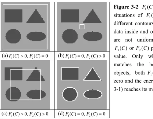
four different combinations which are illustrated in Figure 3-2. In Figure 3-2 (a), the values outside the contour are unique and thusF₂(C)=0. The image data inside the contour contains two distinct values and thus F₁(C)>0. The same analysis can be applied to Figure 3-2 (b). Now the image data outside the contour contains two values and thusF₂(C)>0. If the contour shown in Figure 3-2 (c) passes across the objects, both F₁(C)andF₂(C)are non-zero. When the contours match the boundary of the

(a)F1(C)>0,F2(C)=0 (b)F1(C)=0,F2(C)>0

(c)F1(C)>0,F2(C)>0 (d)F1(C)=0,F2(C)=0

Figure 3-2 F₁(C) and F₂(C). Four

situations of F₁(C)andF₂(C) with

different contours. When the image data inside and outside the contours are not uniform, the values of

) (

1 C

F or F₂(C) produce a positive

value. Only when the contours matches the boundaries of the objects, both F₁(C) and F₂(C) are

zero and the energy function in (Eq. 3-1) reaches its minimum.

The updating equation of the level set function is to be derived from (Eq. 3-1). First we define the Heaviside function H, which is expressed as

⎩ ⎨ ⎧ > ≤ = 0 , 0 0 , 1 ) ( z if z if z H .

If the length of the contours is taken into account, (Eq. 3-1) becomes

∫

∫

Ω − + Ω − − = u x y c H x y dxdy u x y c H x y dxdy E ( , ) ₁ 2 (ϕ( , )) ( , ) ₂ 2(1 (ϕ( , )))

∫

Ω ∇ + H(ϕ(x,y)) dxdy _{(Eq. 3-2)}

The first two terms are the new “without edges” models and the last term represents the length of the contours. According to the geodesic contour model mentioned in Section 2.2, the contour propagates based on the following equation:

(

g C g C N

)

N Ct v v v v v ), ( ) ( − ∇ = κ .

In this case, the weighting g(Cv)=1 and the above equation is simplified to be

N

Cv_t =κ v . (Eq. 3-3)

According to the active region model in Section 2.4, the first two terms in (Eq. 3-2) contribute the propagation force

Outside Inside

t u x y c N u x y c N

(

u(x,y)−c₁ 2 − u(x,y)−c₂ 2

)

Nv

= . (Eq. 3-4)

Combining (Eq. 3-3) and (Eq. 3-4) and applying the level set theory, the updating equation becomes ϕ ϕ ϕ ϕ _∇ ⎥ ⎥ ⎦ ⎤ ⎢ ⎢ ⎣ ⎡ ⎟ ⎟ ⎠ ⎞ ⎜ ⎜ ⎝ ⎛ ∇ ∇ + − − − = u x y c u x y c div t d d 2 2 2 1 ( , ) ) , ( . (Eq. 3-5)

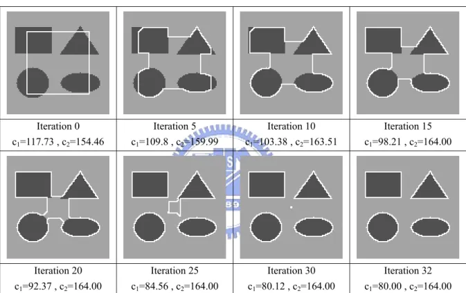
The result of active contours without edges is shown in Figure 3-3.

Iteration 0 c1=117.73 , c2=154.46 Iteration 5 c1=109.8 , c2=159.99 Iteration 10 c1=103.38 , c2=163.51 Iteration 15 c1=98.21 , c2=164.00 Iteration 20 c1=92.37 , c2=164.00 Iteration 25 c1=84.56 , c2=164.00 Iteration 30 c1=80.12 , c2=164.00 Iteration 32 c1=80.00 , c2=164.00

Figure 3-3 Active contours without edges. c1 and c2 are the average values inside and

outside the contours, respectively.

Because there are only two values in the image, the above simple case makes the energy function reach zero. When the image is blurred or added with some noise, the new model may still work well but the energy function reaches a non-zero minimum. Some non-trivial examples will be shown as follows.

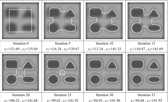
Figure 3-4 shows the contour propagation in a blurred image. The blurred image is filtered by a Gaussian smoothing low-pass filter with the standard deviation 5.

Iteration 0 c1=121.69 , c2=135.69 Iteration 5 c1=116.28 , c2=139.67 Iteration 10 c1=113.24 , c2=141.33 Iteration 15 c1=110.47 , c2=141.69 Iteration 20 c1=106.22 , c2=141.68 Iteration 25 c1=99.62 , c2=141.92 Iteration 30 c1=94.93 , c2=141.96 Iteration 33 c1=94.68 , c2=141.93

Figure 3-4 Apply the “active contours without edges” method to the Gaussian smoothed

image. c1 and c2 are the average values inside and outside the contours,

respectively. Iteration 0 c1=119.17 , c2=152.36 Iteration 5 c1=109.39, c2=160.18 Iteration 10 c1=102.86 , c2=164.27 Iteration 15 c1=98.30 , c2=165.11 Iteration 20 c1=93.14 , c2=165.06 Iteration 25 c1=85.94 , c2=164.91 Iteration 30 c1=80.77 , c2=164.74 Iteration 33 c1=80.39 , c2=164.67

Figure 3-5 Apply the “active contours without edges” approach to the image with

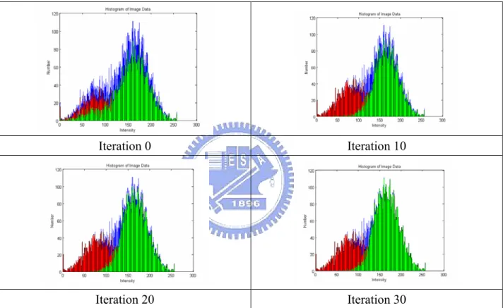
When this model is applied to a noisy image, some defects may appear as shown in Figure 3-5. Because the terms inside the integrals in (Eq. 3-1) are not continuous functions in the image spatial domain, some fragmented contours may be produced by the noise. The variation of the histogram inside and outside the contour is shown in Figure 3-6. It shows that the contours propagate toward the minimum of (Eq. 3-1) in the statistical sense. The blue bar is the histogram of the whole image, the red bar is the histogram of the inside region, and the green bar is the histogram of the outside region. The distributions of the inside and outside regions become more concentrated around the peak of the mean values.

Iteration 0 Iteration 10

Iteration 20 Iteration 30

Figure 3-6 Statistical histogram of Figure 3-5. The blue bar is the histogram of the whole

image, the red bar is the histogram of the inside region, and the green bar is the histogram of the outside region.

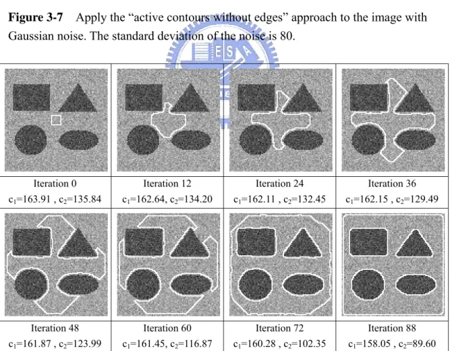
To overcome the defects in Figure 3-5, the input image is pre-filtered by a Gaussian low-pass filter before the contour propagation starts. The result of the pre-filtered noise image is show in Figure 3-7. The standard deviation of the noise is now 80, which is much larger than the case in Figure 3-5.

Iteration 0 c1=119.96 , c2=143.85 Iteration 5 c1=113.08, c2=149.33 Iteration 10 c1=109.00 , c2=151.90 Iteration 15 c1=105.57 , c2=152.18 Iteration 20 c1=101.52 , c2=152.00 Iteration 25 c1=95.32 , c2=151.93 Iteration 30 c1=90.23 , c2=151.79 Iteration 33 c1=90.06 , c2=151.75

Figure 3-7 Apply the “active contours without edges” approach to the image with

Gaussian noise. The standard deviation of the noise is 80.

Iteration 0 c1=163.91 , c2=135.84 Iteration 12 c1=162.64, c2=134.20 Iteration 24 c1=162.11 , c2=132.45 Iteration 36 c1=162.15 , c2=129.49 Iteration 48 c1=161.87 , c2=123.99 Iteration 60 c1=161.45, c2=116.87 Iteration 72 c1=160.28 , c2=102.35 Iteration 88 c1=158.05 , c2=89.60

Figure 3-8 Apply the “active contours without edges” approach to the image with

improper initialization. The standard deviation of the noise is 20. Note that c1 is larger