國
立
交
通
大
學
資訊科學與工程研究所
碩
士
論
文
利 用 圖 形 處 理 器 加 速 鉅 量 多 人
連 線 遊 戲 伺 服 器 端 之 運 算
Using GPU as Co-processor in MMOG Server-side Computing
研 究 生:宋牧奇
利用圖形處理器加速鉅量多人連線遊戲伺服器端之運算
Using GPU as Co-processor in MMOG Server-side Computing
研 究 生:宋牧奇 Student:Mu-Chi Sung
指導教授:袁賢銘 Advisor:Shyan-Ming Yuan
國 立 交 通 大 學
資 訊 科 學 與 工 程 研 究 所
碩 士 論 文
A ThesisSubmitted to Institute of Computer Science and Engineering College of Computer Science
National Chiao Tung University in partial Fulfillment of the Requirements
for the Degree of Master
in
Computer Science
June 2007
Hsinchu, Taiwan, Republic of China
中 華 民 國 九 十 六 年 六 月
利用圖形處理器加速鉅量多人連線遊戲伺服器端之運算 研究生: 宋牧奇 指導教授: 袁賢銘 國立交通大學資訊科學與工程研究所 摘要 一般來說,MMOG(鉅量多人連線遊戲)主要包含了一個廣大的虛擬世界, 容許成千上萬的玩家在這個世界裡進行遊戲以及互動。然而,當我們要設計一個 MMOG 的平台(或中介軟體)來協助遊戲的開發時,我們常常會碰到各式各樣 的瓶頸,限制了在單一平台上最多能容許的玩家人數。本研究探討了這限制之最 根本的原因,就是在 CPU 上循序的處理遊戲邏輯;我們提出了一個革命性的方 法,讓GPU(圖形處理器)來加速這些遊戲邏輯的計算,減低 CPU 的負擔,讓 CPU 更專心於處理 OS 以及 I/O 方面的訊息。 本論文是目前為止第一個利用了 GPU 的計算能力,來加速 MMOG 伺服器 端之運算的研究。我們提出了數個平行的演算法,將用來原本該在 CPU 上之邏 輯運算,轉換成可以在GPU 上平行處理的演算法。在我們的實作中,隨著玩家 人數的增加,我們觀察到在GPU 提供了超過 100 倍目前 CPU 所能提供之運算能 力。搭配適合的IO 架構,在單一伺服器上服務超過 50 萬個玩家即可被實現。Using GPU as Co-processor in MMOG Server-side Computing
Student: Mu-Chi Sung Advisor: Shyan-Ming Yuan
Department of Computer Science and Engineering National Chiao Tung University
Abstract
In general, MMOG (Massively Multiplayer Online Game) consists of virtual worlds where thousands or millions of people can login into the same place and interact with each other. However, when designing a generic MMOG platform to support game development, there are always bottlenecks which limit the maximum number of concurrent players within a single server cluster. In this paper, we identify the source of the limitation, which comes from sequential processing overhead, and propose an innovative approach to solve the scalability problem in parallel by GPU (Graphics Processor Unit).
This is the first research that exploits GPU computation power to accelerate MMOG server-side computing. Several parallel algorithms handling server-side computation of MMOG are derived and implemented on GPU. In our implementation, we observed the performance improvement of GPU is more than 100 times, compared to modern CPU. Together with underlying supporting network communication infrastructure, we build a scalable and high performance MMOG platform that serves up to 500k players on line with a single server at low cost.
Acknowledgement
首先我要感謝袁賢銘教授給我的指導,在我的研究領域裡給予我很多的意見,並 且給予我最大的空間來發揮我的創意。也感謝所有幫助我的學長蕭存喻、葉秉哲, 在我研究的過程中給我不少的指導跟建議。還有感謝我的同學林志達,在一起討 論的過程中激盪出不少的想法。還有所有實驗室內提供電腦給我做實驗的同學, 沒有你們我無法完成實驗。最後我要感謝我的爸媽,給予我這個良好的環境讓我 求學生涯毫無後顧之憂,專心於學業,謹以這篇小小的學術成就來感謝您們的養 育之恩。Table of Contents
Acknowledgement ... v
Table of Contents ... vi
List of Figures ... viii
List of Tables ... x
Chapter 1 Introduction ... 1
1.1. Preface ... 1 1.2. Motivation ... 1 1.3. Problem Description ... 2 1.4. Research Objectives ... 4 1.5. Research Contribution ... 5Chapter 2 Background and Related Work ... 6
2.1. Graphics Processor Unit (GPU) ... 6
2.1.1. From OpenGL to High-Level Shader Language ... 7
2.1.2. Compute Unified Device Architecture (CUDA) by NVIDIA ... 8
2.1.3. Close To Metal (CTM) by AMD/ATI ... 12
Chapter 3 Parallelize the MMOG Server ... 13
3.1. GPU-Assisted MMOG System Architecture ... 13
3.2. Parallel Algorithm on CUDA... 15
3.3. Parallel Logic Processing Algorithm ... 15
3.4. Parallel Conflict Merge Algorithm ... 18
3.5. Parallel Range Query Algorithm ... 24
Chapter 4 Experimental Results and Analysis ... 33
4.1.1. Hardware Configuration ... 34
4.1.2. Software Configuration ... 35
4.2. Evaluation and Analysis ... 36
4.2.1. Comparison of CPU and GPU ... 36
4.2.2. Detail Performance of GPU ... 40
4.2.3. Comparison of CPU and GPU with Computation Only ... 41
4.2.4. Comparison of Different AOIs ... 45
Chapter 5 Conclusions and Future Works ... 47
5.1. Conclusions ... 47
5.2. Future Works ... 48
List of Figures
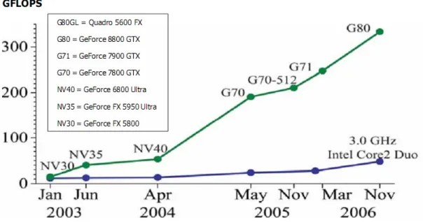
Fig 2-1 Floating-Point Operations per Second for the CPU and GPU ... 6
Fig 2-2 Shared Memory Architecture for GPU ... 9
Fig 2-3 Massively Threaded Architecture ... 10
Fig 2-4 Physical Memory Model on GPU ... 11
Fig 3-1 The count phase of the parallel move logic ... 17
Fig 3-2 The store phase of the parallel move logic ... 18
Fig 3-3 The parallel move logic on GPU ... 18
Fig 3-4 Separation mark for the parallel merge conflict algorithm ... 21
Fig 3-5 Store separation indices for the parallel merge conflict algorithm ... 21
Fig 3-6 Merge conflict intervals for the parallel merge conflict algorithm ... 22
Fig 3-7 The parallel merge conflict algorithm ... 23
Fig 3-8 Multiple update ranges in a grid ... 25
Fig 3-9 Write affected bucket indices for the parallel range query algorithm ... 27
Fig 3-10 Mark separation for the parallel range query algorithm ... 28
Fig 3-11 Store separation indices for the parallel range query algorithm ... 29
Fig 3-12 The two-way binary search in the parallel range query algorithm ... 30
Fig 3-13 Count the number of updates for the parallel range query algorithm ... 31
Fig 3-14 Enumerate the updates for the parallel range query algorithm ... 31
Fig 3-15 The parallel range query algorithm ... 32
Fig 4-1 Average Execution Time for map size 2500x2500 ... 37
Fig 4-2 Average Execution Time for map size 5000x5000 ... 38
Fig 4-3 Performance Improvement Ratio of GPU over CPU ... 39 Fig 4-4 Average Execution Time for map size 2500x2500 (GPU w/ Computation Only)
... 42 Fig 4-5 Average Execution Time for map size 5000x5000 (GPU w/ Computation Only)
... 43 Fig 4-3 Performance Improvement Ratio of GPU over CPU (GPU w/ Computation
List of Tables
Table 2-1 Memory Addressing Spaces available on CUDA ... 10
Table 4-1 Hardware Configuration ... 34
Table 4-2 NVIDIA 8800GTX Hardware Specification ... 34
Table 4-3 Software Configuration ... 35
Table 4-4 Tested Scenarios ... 36
Table 4-5 Average Execution Time for map size 2500x2500 ... 37
Table 4-6 Average Execution Time for map size 5000x5000 ... 38
Table 4-7 Performance Improvement Ratio of GPU over CPU ... 39
Table 4-8 Detailed Execution Time of GPU Algorithm at Each Step ... 41
Table 4-9 Average Time for map size 2500x2500 (GPU w/ Computation Only) ... 42
Table 4-10 Average Time for map size 5000x5000 (GPU w/ Computation Only) ... 43
Table 4-11 Performance Improvement Ratio of GPU over CPU (GPU w/ Computation Only) ... 44
Chapter 1 Introduction
1.1. Preface
MMOG (Massively Multiplayer Online Game) could be the biggest revolution in computer game industry in recent years. As network technology evolved rapidly, thousands or millions of people can login into the same virtual world, stand at the same position, and play the same game together just like they are virtually in the same room at the same place. This has been such a great success since Korea became the world largest exporter of online games in the year of 2002, and it is now a billion-scale global market expected to continue its impressive growth.
1.2. Motivation
However, right now, it takes at least three two to three years and $20 million USD to build a MMOG, due to challenges in the areas of engineering, asset-creation, and marketing. For engineering, to build an enterprise-level network infrastructure that can scale to millions of simultaneous users would be daunting for almost any game developer. It’s basically outside their area of interest and expertise. As a result, numbers of middleware solutions for game developers to ease the development cost for MMOG has shown up since the year of 2004. Also, several open-source projects have been created to provide free solution. It seems like they all try to answer to the question about MMOG scalability and flexibility and to claim the significantly benefit that hide the complexities of server through the provided platforms.
Although there’s no in-depth comparison among all of them, from the titles that are based on these middleware solutions, we observed that the scalabilities of these
platforms are not as good as what we expected to see. As the real-world game designs are so complicated that make a great impact on server performances, the average number of concurrent online players falls in the range between 2000 and 9000 per server cluster, which is consist of 5 to 20 servers (so each server is only capable of 500~1000 players). For such limitation, most virtual game worlds are replicated into several independent worlds (called shards), in which players cannot communicate with each other due to the geographical constraint. To address the shard problem, recently the Project Darkstar initiated by Sun Microsystems announced their new technology to build “shardless” MMOGs. However the number of concurrent players per server is still low and therefore the cost for entire server cluster remains high. Also, their shardless technology is based on dynamic allocation on pre-defined fixed game region, which limits the provisioning efficiency due to the synchronization overhead of those mirror servers.
We looked into the scalability problem in most of the commercial off-the-shelf MMOG platforms as well as the open source ones, and tried to propose a solution that can really scale up to a very large number of concurrent players on a single server.
1.3. Problem Description
Designing a reusable, flexible, easy-to-use MMOG platform is challenging. Despite of the usability, the performance metrics are also significant, such as the scalability of MMOG. Scalability is usually the key to operating cost, because the higher scalability the platform is, the lower machine needed to be deployed, which results in lower cost.
maximum number of concurrent players ever recorded is 22020. Other than that, as mentioned above, most of each server cluster ranges from 2000 to 9000. As far as we are concern, this is a relatively poor record compared to other internet service such as web server.
To see why, we need to know that the design constraints of MMOG platforms are unique, that is, tens of thousands or millions of players log in the same virtual world to interact with each other, and results in an aggressive amount of commands and updates generated as players move and attack. Therefore, the server cluster needs to process all the commands and sends all the updates to players within a limited time constraint. Lots of researchers put their eye on reducing the network latency to give more time to serve requests. The proposed communication architectures include peer-to-peer architecture and the scalable server/proxy architecture. They all succeed to reduce the network latency to have more concurrent players within acceptable time delay; however the maximum concurrent players is still far from 10k, which is the capability that a scalable server should have generally. There should be some other bottleneck in the design.
In our point of view, since the network technology evolved rapidly that the optical interconnection is popping out of the surface and the broadband internet access is becoming the majority, the transmission delay between the server and the client has dropped to a certain level. Eventually, the network latency will not be an issue in the near future, and we will spend the most of processing time for client commands. Basically, due to the current CPU architecture, CPU is not capable of large amount of data, which is most likely the case of MMOG. Although multi-core CPU has come to market, the memory bandwidth between CPU and main memory is still low, and multiple cache-misses occurred for the sake of limited resources and different
execution contexts of the game logics and network handlers. Also, different thread executions need synchronization and atomic locking operation to avoid update conflicts. Apparently, these constraints damage the performance and limit the throughput of executing client commands on CPU.
1.4. Research Objectives
As we identify the kernel of the problem is due to the architecture of CPU, we began to search for methods to efficiently process significant amount the client commands and update the entire virtual world. Our final answer is GPU. For last decade, GPU has been transformed from a simple 3D rendering acceleration silicon into an array of SIMD processors [3]. According to survey, the computation power of GPU is more than 100 times than CPU, and also, the memory bandwidth between the processor and the device memory of GPU is much larger than that of CPU. In general, GPU has been specialized for both compute-intensive and highly parallel computation, and the computation power of GPU has been grown rapidly even beyond Moore’s Law [4]. From the year of 2003, some researcher began to make use of GPU to do general purpose computation by mapping the general purpose problems into a 3D rendering problems. These problems range from collision detection [5] to online databases [6]. In all of the studies, the performance boost by 10 to 100 times is observed by exploiting GPU computation.
However, until now, none work has been done toward applying GPU to MMOG platform design. The most possible reason for that could be the complicated calculation and update conflict problem in the MMOG platform. But with the latest evolution of GPU technology, which will be discussed on the next chapter, it seems like GPU is ready and will become a possible choice to migrate the computation load
from CPU to GPU.
To summarize, as discussed above, for the reason that the computation problem in MMOG is computation-intensive and highly data-parallel, we want to apply GPU to general purpose computation on MMOG platform to reduce the overhead in logic processing and game world updates.
1.5. Research Contribution
This thesis discussed the issue of the barrier to build a MMOG server on GPU and proposed a practical solution and system on GPU to handle all client commands and updates. Based on different programming paradigm (sequential vs. parallel), the MMOG server needs to be re-designed to parallelize all works on GPU. New algorithms specialized to process client commands in parallel and to update the virtual world with respect to update conflicts are proposed.
Chapter 2 Background and Related Work
2.1. Graphics Processor Unit (GPU)
As mentioned above, the GPU technology changed a lot in both hardware and software in the last decade. In hardware, fixed-function rendering pipeline is obsolete and new programmable pipeline consist of multiple SIMD processor is a de facto standard in the GPU industry. The comparison of computation power between GPU and CPU was depicted as Fig 2-1. As for software, the OpenGL persists, but many extensions have been added by the OpenGL ARB to facilitate the use of programmable pipeline. Based on the programmable pipeline and the SIMD architecture of current GPU, one can map a compute-intensive problem into multiple small pieces, solve the problem within a pixel-rendering context (because the pixel rendering is programmable), and finally store the result in the frame buffer object. This is the basic concept of general purpose computation on graphics hardware, also called GPGPU [7] [8].
However the mapping is not straightforward, we may need to design some special data structure and modify the algorithm in the way we do graphics rendering. Fortunately, the two biggest GPU manufacturers: NVIDIA and AMD/ATI have just opened the computation power to public via some programming interface other than OpenGL, which we will introduce later.
2.1.1. From OpenGL to High-Level Shader Language
Before digging into the latest development of GPU programming, we give the history of OpenGL first to get better understanding of the benefit from the new programming architecture.
OpenGL was developed by SGI in early 90s to standardized access to graphics hardware, and ease the development of 3D computer graphics by providing high-level and simple set of APIs. Since 90s, there are several revisions of OpenGL to adopt new graphics hardware. Among all the revision, the most important one is the standard of OpenGL 2.0, in which the OpenGL Shading Language [10], GLSL for short, is introduced. GLSL provides high level construct to write shader, which is the program that is executed on each vertex or pixel is rendered. As long as we can encapsulate the data into textures, and transform the work into numbers of independent pixel renderings, the problem can be executed in parallel on GPU.
However, shader comes with limits since GPU is not designed under the same principle of CPU. You can never arbitrarily write to any memory location but only the corresponding output pixel in a shader. This is known scatter write operation, which is prohibited on GPU because read-after-write hazard would occur to damage the GPU performance if such operation is allowed. Under these constraints, GPU algorithms are even harder to be developed then traditional algorithm and was turned into a very active research field in the last few years.
In addition, NVIDIA proposed Cg in 2003 to further lower the burden of GLSL by providing C standard language construct to write shaders. However the Cg itself does not manipulate the graphics hardware directly, but instead, they transform Cg codes into standard GLSL code by compiler techniques; as a result, Cg does not relief the constraint on GPU but only providing a friendly and easy-to-use development environment.
2.1.2. Compute Unified Device Architecture (CUDA) by NVIDIA
CUDA, as the name stands for, is the architecture to unify the general computation model on graphics devices. Just like the Cg they invented previously, CUDA uses standard C language with some simple extensions such as templates and C++ style variable declaration. This gives programmer a great convenient to develop GPU application. From now on, we will introduce to CUDA in more detail because we will use CUDA to implement the entire system, and CUDA is much different from OpenGL or any other popular programming language in many perspectives.
The most important advantage of CUDA over graphics API for making traditional general computation on GPU is the scattered write capability. To explain, scattered write means that code written in CUDA can write to arbitrary addresses in memory, which is not possible in traditional pixel shader programming (unless combined with the vertex shader, but this is extremely inefficient). CUDA provides scatter write to make many parallel algorithm possible to be implemented on GPU, such as parallel prefix sum algorithm (also called the SCAN operation) and efficient bitonic sort.
Fig 2-2 Shared Memory Architecture for GPU
Along with scatter write, CUDA further exposed a fast shared memory on GPU that can be shared among numbers of processors as Fig 2-2. The shared memory can be used as a user-managed cache, enabling extreme high bandwidth than traditional texture look up, which is actually accessing global memory. Furthermore, as stated in the CUDA official document, when programmed through CUDA, GPU is viewed as a compute device that is capable of executing a very high number of threads in parallel as Fig 2-3. This is called massively threaded architecture. To explain further, each kernel can be executed by a grid of blocks, and each block contains a grid of thread that is conceptually mapped to a single SIMD processor. Threads within the same block can communicate with each other via per-block shared memory and get synchronized at a specific point of execution. A Block can be regarded as a set of threads within the same execution context. However, unlike thread, there is no synchronization capability among blocks.
Fig 2-3 Massively Threaded Architecture
As for the memory model of CUDA, there’s six different types of memory that can be access either in read-write mode or in read-only mode, summarized as follows:
Name Accessibility Scope Speed Cache Registers read/write per-thread zero delay (on chip) X
Local Memory read/write per-thread DRAM N
Shared Memory read/write per-block zero delay (on chip)* N
Global Memory read/write per grid DRAM N
Constant Memory read only per-grid DRAM Y
Texture Memory read only per-grid DRAM Y
Table 2-1 Memory Addressing Spaces available on CUDA
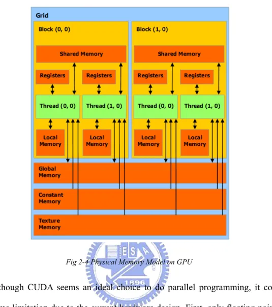
Along with , Fig 2-4 shows the graphical layout of memory on GPU. In fact, there are only two types of memory physically on GPU: the on-chip memory and the device memory, but they are divided into different memory spaces for different purposes of use. The on-chip memory is embedded in the SIMD processor that only 2 clocks needed to read from or write to. The access to device memory usually takes up to 200~300 clocks, which is relatively slow compared to on-chip memory. The shared memory located on the chip can be regarded as a user-managed cache for the SIMD processor. A typical usage of shared memory is used to cache specific data read from global memory to avoid duplicate read. Also, shared memory can be served as an inter-process communication medium for all threads with almost zero overhead.
Fig 2-4 Physical Memory Model on GPU
Although CUDA seems an ideal choice to do parallel programming, it comes with some limitation due to the current hardware design. First, only floating point of single precision is supported no current hardware; applications that require double precision floating point computation are not viable. Second, recursive function is not supported due to the lack of stack on GPU. Third, the branching within the same block could be expensive as they are executed on a SIMD processor, where only one instruction can be performed (with multiple different data source) at one time. So if threads take different execution path, they must be serialized by the thread scheduler on GPU. Finally, while GPU is communicated with CPU through the PCI-Express bus, the cost to download/upload data from/to GPU would be expensive. As a result, frequent data transfer between CPU and GPU should be avoided whenever possible. For more details about CUDA, please refer to the CUDA programming guide [11].
2.1.3. Close To Metal (CTM) by AMD/ATI
Compared to NVIDIA CUDA, the second largest GPU manufacturer announced the Close To Metal (CTM) [12] technology before CUDA. With similar goal of CUDA, CTM try to expose the computation power of GPU for the public to apply GPU to general purpose computation. However, in a very different approach from CUDA, CTM does not provide the comprehensive toolkits like compiler, linker and high-level C language construct, but only a set of low-level, assembly-like, raw commands that is executable by AMD/ATI’s GPU. This is really daunting for most developers. Therefore, till now, CTM does not attract much attention although CTM almost covers all aspect of what CUDA can do.
Chapter 3 Parallelize the MMOG Server
In this chapter, we propose the GPU-assisted MMOG server design, which mixes the unparallel processing power of GPU with the component-based MMOG server architecture. We will later describe our parallel MMOG algorithms on CUDA, including parallel logic processing algorithm and parallel range query/update algorithm.
3.1. GPU-Assisted MMOG System Architecture
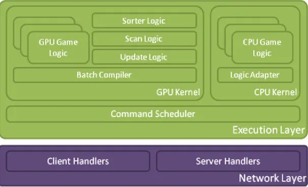
Fig 3-1 the logic execution layer of GPU-assisted MMOG system
The entire GPU-assisted MMOG system framework was depicted in Fig 3-1. Basically, the framework can be stratified into 3 layers by their functionalities: the network layer, the control layer, and the execution layer.
Network layer provides reliable unicast and multicast transport to assist inter-process communication in the online game network. With modern high
performance and fault-tolerant communication middleware and gateway/server architecture, we can handle massive amount client requests and exchange data among servers efficiently.
Execution layer, which is the kernel of the system, handles all client commands received from network layer and dispatch all commands to corresponding logic (i.e. handler) according to the types of the commands. To maximize the number of concurrent users, we used GPU to assist the logic computation on server based on NVIDIA CUDA framework.
To elaborate, basically clients interact with servers based on well-known server/gateway architecture as follows. First, the client sends corresponding commands to the proxy he connected to, as the player manipulates his/her character. Upon the arrival of the client command, the proxy relays the command along with those from other clients to the game server. The game server collects all client commands, compiles into request list, and uploads to GPU memory. GPU then processes client commands by a great number of blocks of threads, updates the game world in parallel, and finally compiles the update vectors into a continuous array. Next, update vectors are downloaded to CPU memory. By the update vectors, clients that are affected by the changes of the world need to be notified by sending player state updates via the corresponding proxies. Each proxy will then forward the state updates to clients and finally the result is rendered on clients’ display.
3.2. Parallel Algorithm on CUDA
For most parallel algorithm, the parallel sorting and parallel prefix sum algorithm are the basic building essential. As a result, we implemented load balanced parallel radix sort [16] and parallel prefix sum [17], and optimized it according to the GPU architecture constraints.
For implementation, due to the bandwidth limit between GPU memory and host memory in current commodity computers, we must avoid data transfer as much as possible to get the best performance. For that reason, we try to process the client commands and virtual world updates completely on GPU. Client commands are compiled as a request array and sent to GPU by command scheduler. Next, GPU will process all client commands in the request array in parallel, merge all update conflicts, identify those who are near these altered players by bucket indices, and finally generate the update array. The update array will be read back from GPU memory to CPU memory and be processed by CPU. Each item in the update array is a vector consists of the player id to send update, the altered player id, the altered data id, and the new value of the data. CPU will send the altered player state update to the nearby player according to the update vector.
3.3. Parallel Logic Processing Algorithm
As processing client commands on GPU, we must store the player information needed during the execution of logic. Since the GPU memory size is limited, we only store a part of data of player states relevant to GPU game logics. For example, we may need to store the position of players as a small chunk on GPU if we have the move logic on GPU.
Logic on GPU can be regarded as a set of chunk update rules, that is, it might request to modify a number of chunks in player states according to predefined rules by writing a list of update vector of player id, chunk id, and value offset. Note that there could be multiple update vectors toward the same player id with the same chunk id, which lead to conflicts. We will introduce the parallel update conflict merge algorithm to address the problem in the next section.
However to make the logic processing parallel is not that straightforward. To make it parallel, we need to split all logics into two phases, the counting phase and storing phase. In the counting phase of the specific logic, we compute the number of updates that will be generated in the logic and store the update count into global memory on GPU by each thread. After that, we perform parallel prefix sum to calculate the exact memory location to store all update vectors in a continuous block of memory. Given the memory locations, the storing phase of the logic is then performed and writing all updates to global memory without any address conflict.
For example, suppose we have an attack logic implemented on GPU, different update counts will be stored by each thread in the update count array. For example, 5 updates for thread 1 will be generated later, 3 updates for thread 2, and 1 update for thread 3. The update count array will look like {5, 3, 1, …}. After parallel prefix sum is applied, the update count array becomes {0, 5, 8, 9, …}, in which each element is exactly the sum of all elements before. Based on the prefixed update count, each thread can safely store the update vectors into global memory without write-after-write hazards.
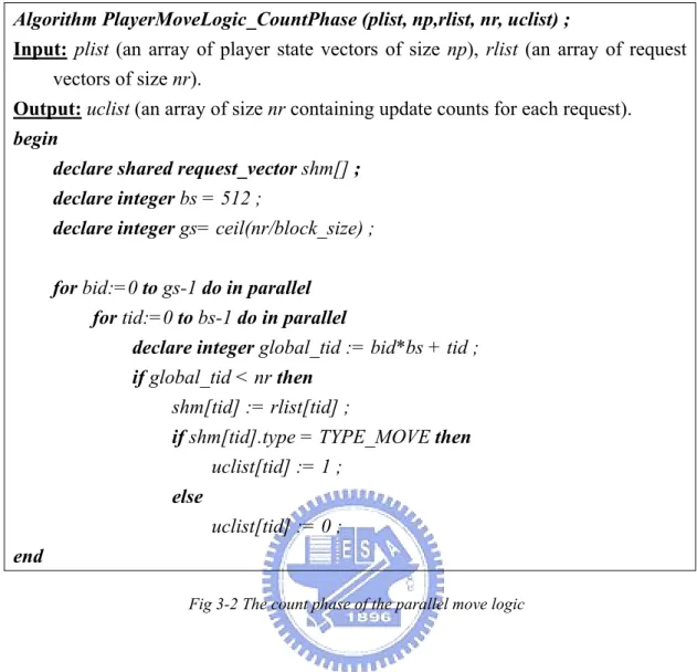
Although game logics are designed based on the game’s philosophy, we implemented the simple move logic to demonstrate the two-phase concept as in Fig 3-2, Fig 3-3, and Fig 3-4
Algorithm PlayerMoveLogic_CountPhase (plist, np,rlist, nr, uclist) ;
Input: plist (an array of player state vectors of size np), rlist (an array of request
vectors of size nr).
Output: uclist (an array of size nr containing update counts for each request).
begin
declare shared request_vector shm[] ; declare integer bs = 512 ;
declare integer gs= ceil(nr/block_size) ;
for bid:=0 to gs-1 do in parallel for tid:=0 to bs-1 do in parallel
declare integer global_tid := bid*bs + tid ; if global_tid < nr then
shm[tid] := rlist[tid] ;
if shm[tid].type = TYPE_MOVE then
uclist[tid] := 1 ;
else
uclist[tid] := 0 ;
end
Fig 3-2 The count phase of the parallel move logic
Algorithm PlayerMoveLogic_StorePhase (plist, np, rlist, nr, uslist, ulist) ;
Input: plist (an array of player state vectors of size np), rlist (an array of request
vectors of size nr), uslist (an array of indices where each thread stores the updates).
Output: ulist (an array of update vectors of size nr).
begin
declare shared request_vector shm[] ; declare integer bs := 512 ;
declare integer gs := ceil(nr/block_size) ;
for bid:=0 to gs-1 do in parallel for tid:=0 to bs-1 do in parallel
declare integer global_tid := bid*bs + tid ; if global_tid < nr then
if shm[tid].type = TYPE_MOVE then declare update_vector upd ;
upd.playerID := shm[tid].playerID ;
upd.chunkID := PLAYER_POSITION ;
upd.offset := calculateOffset(shm[tid]) ;
ulist[uslist[tid]] := upd ;
end
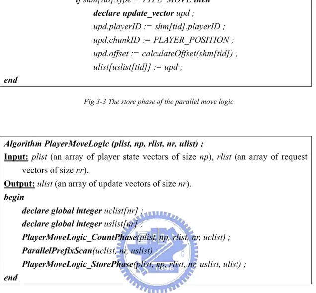
Fig 3-3 The store phase of the parallel move logic
Algorithm PlayerMoveLogic (plist, np, rlist, nr, ulist) ;
Input: plist (an array of player state vectors of size np), rlist (an array of request
vectors of size nr).
Output: ulist (an array of update vectors of size nr).
begin
declare global integer uclist[nr] ; declare global integer uslist[nr] ;
PlayerMoveLogic_CountPhase(plist, np, rlist, nr, uclist) ; ParallelPrefixScan(uclist, nr, uslist) ;
PlayerMoveLogic_StorePhase(plist, np, rlist, nr, uslist, ulist) ; end
Fig 3-4 The parallel move logic on GPU
3.4. Parallel Conflict Merge Algorithm
As mentioned above, there may be update conflicts in the update vectors generated by game logics. To address the problem, we propose the parallel update conflict merge algorithm to merge conflict updates into one conflict-free update. For example, when more than one player is attacking someone else, there will be multiple attack commands in a single update iteration requested by different player, but their targets are same. In this case, multiple update vectors will be generated by different threads and stored in the update array. We have to find out all those conflict updates and sum up all their offsets as one, and replace all update vectors by the new update
vector.
The algorithm works as follows. In the first step, we need to sort the list of update vectors in parallel according to their player id and chunk id. Ultimately, we want to find out the interval to merge on the sorted list. Therefore, we check each interval between any two adjacent elements in the sorted list to see if the left and the right elements are in conflict with each other. We call this separation marking. If the left and the right elements are conflict-free, then 1 is written to the separation list as a separation mark. Otherwise, 0 is written. After the separation list is filled out, all update vectors in-between two 1 marks will need to be merged. To find out all the memory address to write those conflict-free update vectors, the parallel prefix sum is performed on the separation list to get the store indices for separation. Given the separation list and the store indices list, we can easily transform the separation marks into the intervals to merge. Take an example; if the sorted vectors are as follows (each vector is in the form {player id, chunk id, value, offset}):
{ { player 0, PLAYER_HP, 100, -5 }, { player 0, PLAYER_HP, 100, -10 }, { player 1, PLAYER_HP, 250, -20 }, { player 2, PLAYER_HP, 300, -30 }, { player 2, PLAYER_HP, 300, -50 }, { player 3, PLAYER_HP, 100, -5 }}
The resulting separation list will be {0, 1, 1, 0, 1}, and after prefix scanned, the store indices list becomes {0, 0, 1, 2, 2}. We spawn a thread on each element of separation list to generate the merge list. Each thread check the corresponding element and write the current thread index to global memory at the location specified in the store indices list in case that corresponding element equals to 1, which is a separation mark. After the transformation, we will have the merge list like {1, 2, 4}.
The final step is to perform parallel merge on the sorted list of update vectors according to merge list. Following the last example, given the merge list {1, 2, 4}, we need to merge {[0, 1], [2, 2], [3, 4]}. We can use one thread for each interval between two adjacent elements in the merge list to sum up all the offsets in-between.
Algorithm MergeConflict_MarkSeperation (ulist, nu, seplist) ;
Input: ulist (an array of update vectors of size nu). Output: seplist (an array of indices of size nu).
begin
declare shared update_vector shm[] ; declare integer bs := 256 ;
declare integer gs := ceil(nu/bs) ;
for bid:=0 to gs-1 do in parallel for tid:=0 to bs-1 do in parallel
declare integer global_tid := bid*bs + tid ; if global_tid < nr then shm[tid] := ulist[tid] ; declare update_vector tl, tr ; synchronize_threads() ; if global_tid < nu then tl := shm[tid] ; synchronize_threads() ;
if global_tid < nu && (tid != bs-1 or bid != gs -1) then if tid = block_size-1 then
tr := ulist[global_tid+1] ;
else
tr := shm[tid+1] ;
declare integer mark := 0 ;
if tl.playerID = tr.playerID && tl.chunkID = tr.chunkID then
mark := 1 ;
if global_tid < nu then
seplist[global_tid] := mark ;
end
Fig 3-5 Separation mark for the parallel merge conflict algorithm
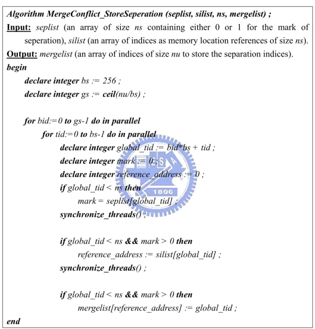
Algorithm MergeConflict_StoreSeperation (seplist, silist, ns, mergelist) ;
Input: seplist (an array of size ns containing either 0 or 1 for the mark of
seperation), silist (an array of indices as memory location references of size ns).
Output: mergelist (an array of indices of size nu to store the separation indices).
begin
declare integer bs := 256 ;
declare integer gs := ceil(nu/bs) ;
for bid:=0 to gs-1 do in parallel for tid:=0 to bs-1 do in parallel
declare integer global_tid := bid*bs + tid ; declare integer mark := 0 ;
declare integer reference_address := 0 ; if global_tid < ns then
mark = seplist[global_tid] ;
synchronize_threads() ;
if global_tid < ns && mark > 0 then
reference_address := silist[global_tid] ;
synchronize_threads() ;
if global_tid < ns && mark > 0 then
mergelist[reference_address] := global_tid ;
end
Fig 3-6 Store separation indices for the parallel merge conflict algorithm
template < class T>
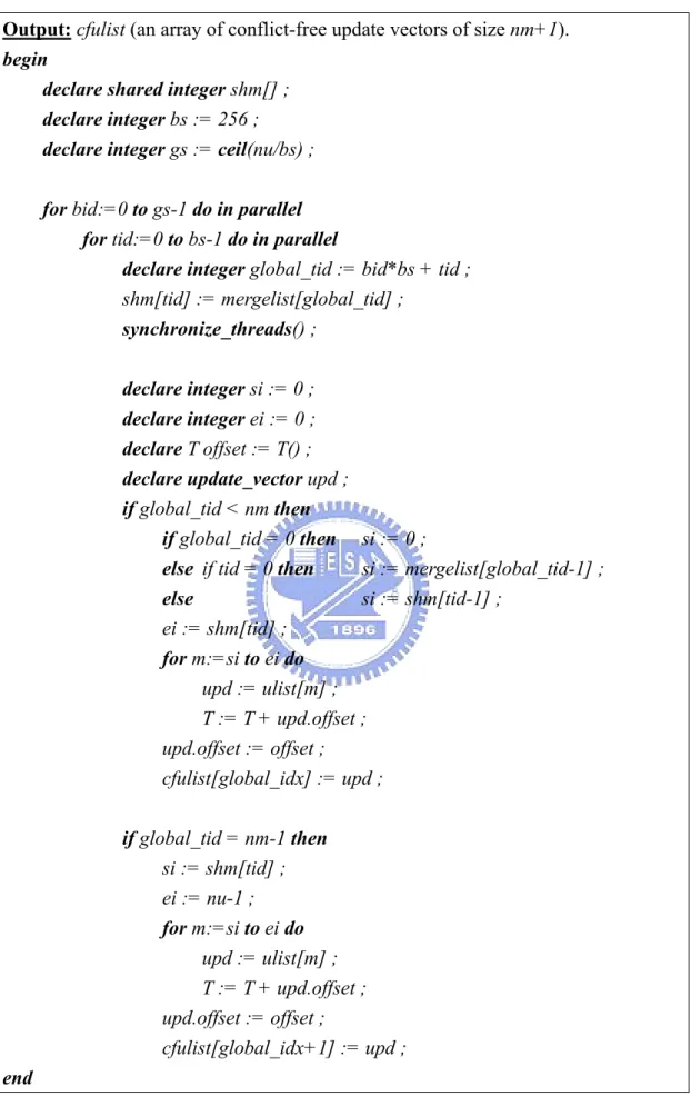
Algorithm MergeConflict_MergeInterval (ulist, nu, mergelist, nm, cfulist) ;
Input: ulist (an array of update vectors of size nu), mergelist (an array of separation
Output: cfulist (an array of conflict-free update vectors of size nm+1).
begin
declare shared integer shm[] ; declare integer bs := 256 ;
declare integer gs := ceil(nu/bs) ;
for bid:=0 to gs-1 do in parallel for tid:=0 to bs-1 do in parallel
declare integer global_tid := bid*bs + tid ;
shm[tid] := mergelist[global_tid] ;
synchronize_threads() ;
declare integer si := 0 ; declare integer ei := 0 ; declare T offset := T() ; declare update_vector upd ; if global_tid < nm then
if global_tid = 0 then si := 0 ;
else if tid = 0 then si := mergelist[global_tid-1] ;
else si := shm[tid-1] ; ei := shm[tid] ; for m:=si to ei do upd := ulist[m] ; T := T + upd.offset ; upd.offset := offset ; cfulist[global_idx] := upd ; if global_tid = nm-1 then si := shm[tid] ; ei := nu-1 ; for m:=si to ei do upd := ulist[m] ; T := T + upd.offset ; upd.offset := offset ; cfulist[global_idx+1] := upd ; end
Algorithm MergeConflict (ulist, nu, cfulist) ;
Input: ulist (an array of update vectors of size nu).
Output: cfulist (an array of conflict-free update vectors of size nu).
begin
declare global update_vector ulist_sort[nu] ; declare global integer seplist[nu] ;
declare global integer silist[nu] ;
ParallelLoadBalancedRadixSort(ulist, nu, ulist_sort) ; MergeConflict_MarkSeperation(ulist_sort, nu, seplist) ; ParallelPrefixScan(seplist, nu, silist) ;
declare integer nm := silist[nu-1] ; declare global integer mergelist[nm] ;
MergeConflict_StoreSeperation(seplist, silist, nu, mergelist) ; MergeConflict_MergeInterval(ulist, nu, mergelist, nm, cfulist) ; End
3.5. Parallel Range Query Algorithm
After those conflict-free update vectors are computed for each client commands, we need to update the virtual world by range search, which is the most time-consuming problem overall. From history, we see that the range search problem has been extensively studied for more than twenty years. Many spatial partitioning methods are proposed to accelerate the neighbor search, such as the quad/oct-tree, range tree, R*-tree…, etc. Most of them are based on pointer to build up the structure of the tree. However this can hardly be done on current GPU due to the limited instruction set and fixed memory model. In [18], Paul uses well-separated pair decomposition to make parallel all-nearest-neighbors search optimal. Since it requires recursion during tree construction and pair computation, it is not feasible on current GPU even the CUDA is used. As a result, we derive our parallel range query algorithm which can be efficiently executed on massively parallel processors with respect to CUDA constraints.
We first assume the visibility range is fixed among all players to simplify the problem, although the limitation can be relaxed by appending a parallel filtering function in the end of the query. Once the range is fixed, we can disperse players into a 2D or 3D grid according to their position in Cartesian space. Grid can be seen as a list of indexed buckets, which is defined as square/cube with edge length equal to the fixed visibility range. This is just the well-known quad/oct-tree data structure. However, since pointer can hardly be implemented and the number of the players in each bucket varies, we cannot store the grid directly on GPU. For example, a straightforward approach is to define the maximum number of players per bucket and reserve all space for every bucket in the grid. Nevertheless, this is a waste in memory, and if the grid size grows larger, GPU will definitely run out of memory in the end
because the GPU memory is relatively small to current CPU1. To save the memory from wasting while preserving the efficiency of range query on GPU, we re-designed the data representation and search algorithm, which will be explained as follows.
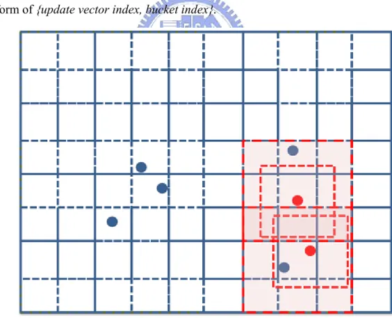
We still rely on the bucket concept in quad/oct-tree to assort all the players. But this time, we store all players’ reference in a continuous array sorted by their bucket indices. This can be efficiently done on GPU by parallel load balanced radix sort. Following that representation, we need to perform range query for neighbors of each player whose state is modified by the game logic. Inspired by discrete method [19] by Takahiro, we defined bucket as square/cube with edge length equal to the visibility range, and for each update vector, we only need to enumerate all players in adjacent buckets as in Fig 3-9. So finally, we have the affected bucket list composed by pairs in the form of {update vector index, bucket index}.
Fig 3-9 Multiple update ranges in a grid
As we stored all players’ reference in a continuous way, there are no direct indices can be used to find out who are the players in the specific bucket. Here we employed the parallel binary search to identify the range of specific bucket, that is, we perform binary search for multiple target keys in the same time. Also, to reduce the number of search times, we extract distinct bucket indices from the affected bucket list by the similar way in resolving update conflicts. The algorithms are illustrated as Fig 3-10, Fig 3-11, and Fig 3-12.
Once we have all needed bucket ranges, we can enumerate all state updates for all adjacent buckets in parallel. Note that before the enumeration, we have to count the number of possible state updates to make sure all updates write to correct memory location in a continuous way. Details about the algorithm can be found in Fig 3-13 to Fig 3-16.
Algorithm ParallelRangeQuery_WriteAffectedBuckets (plist, np, ulist, nu, blist) ;
Input: ulist (an array of update vectors of size nu).
Output: blist (an array of bucket update vector of size nu).
begin
declare shared update_vector shm[] ; declare integer bs := 256 ;
declare integer gs := ceil(nu/bs) ;
for bid:=0 to gs-1 do in parallel for tid:=0 to bs-1 do in parallel
declare integer global_tid := bid*bs + tid ; if global_tid < nu then
declare update_vector upd := ulist[global_tid] ;
declare float2 pos := plist[upd.playerID].position ;
declare int bucket_idx := POSITION_TO_BUCKET_IDX(pos) ; declare integer base := global_tid*9;
declare bucket_update_vector bupd;
bupd.updateID := global_tid;
bupd.bucketID := bucket_idx;
bupd.bucketID := bucket_idx-1; blist[base+1] := bupd; bupd.bucketID := bucket_idx+1; blist[base+2] := bupd; bupd.bucketID := bucket_idx-ROW_SIZE; blist[base+3] := bupd; bupd.bucketID := bucket_idx-ROW_SIZE-1; blist[base+4] := bupd; bupd.bucketID := bucket_idx-ROW_SIZE+1; blist[base+5] := bupd; bupd.bucketID := bucket_idx+ROW_SIZE; blist[base+6] := bupd; bupd.bucketID := bucket_idx+ROW_SIZE-1; blist[base+7] := bupd; bupd.bucketID := bucket_idx+ROW_SIZE+1; blist[base+8] := bupd; end
Fig 3-10 Write affected bucket indices for the parallel range query algorithm
Algorithm ParallelRangeQuery_MarkSeperation (ulist, nu, seplist) ;
Input: ulist (an array of update vectors of size nu). Output: seplist (an array of indices of size nu).
begin
declare shared update_vector shm[] ; declare integer bs := 256 ;
declare integer gs := ceil(nu/bs) ;
for bid:=0 to gs-1 do in parallel for tid:=0 to bs-1 do in parallel
declare integer global_tid := bid*bs + tid ; if global_tid < nr then
shm[tid] := ulist[tid] ;
declare update_vector tl, tr ; synchronize_threads() ;
tl := shm[tid] ;
synchronize_threads() ;
if global_tid < nu && (tid != bs-1 or bid != gs -1) then if tid = block_size-1 then
tr := ulist[global_tid+1] ;
else
tr := shm[tid+1] ;
declare integer mark := 0 ;
if tl.playerID = tr.playerID && tl.chunkID = tr.chunkID then
mark := 1 ;
synchronize_threads() ;
if global_tid < nu then
seplist[global_tid] := mark ;
end
Fig 3-11 Mark separation for the parallel range query algorithm
Algorithm ParallelRangeQuery_StoreSeperation (seplist, silist, ns, dblist) ;
Input: seplist (an array of size ns containing either 0 or 1 for the mark of
seperation), silist (an array of indices as memory location references of size ns).
Output: dblist (an array of indices of size nu to store the distinct indices).
begin
declare integer bs := 256 ;
declare integer gs := ceil(nu/bs) ;
for bid:=0 to gs-1 do in parallel for tid:=0 to bs-1 do in parallel
declare integer global_tid := bid*bs + tid ; declare integer mark := 0 ;
declare integer reference_address := 0 ; if global_tid < ns then
mark := seplist[global_tid] ;
if global_tid < ns && mark > 0 then
reference_address := silist[global_tid] ;
synchronize_threads() ;
if global_tid < ns && mark > 0 then
mergelist[reference_address] := global_tid ;
end
Fig 3-12 Store separation indices for the parallel range query algorithm
Algorithm ParallelRangeQuery_BinarySearch (plist_sort, np, dblist, nb, dbilist) ;
Input: plist_sort (a sorted array of player bucket vector of size np), dblist (an array
of distinct bucket indices of size nb).
Output: dbrlist (an array of bucket ranges of size nb to store the start/end indices of
a specific bucket).
begin
declare integer bs := 256 ;
declare integer gs := ceil(nu/bs) ;
for bid:=0 to gs-1 do in parallel for tid:=0 to bs-1 do in parallel
declare integer global_tid := bid*bs + tid ; if global_tid < nb then
declare player_bucket pl ; declare player_bucket pr ; declare bucket_range range ;
declare integer bucket_idx := dblist[global_tid] ; declare integer rl := np / 2 - 1 ;
declare integer rr := np / 2 - 1 ; declare integer level := np / 2 ; declare integer found := 0 ; do
level := level / 2 ;
pl := plist_sort[rl] ;
if rl = rr then pr := pl ;
if pl = bucket_idx or pr = bucket_idx then found := 1 ;
if pl.bucket <= bucket_idx then rl := rl + level ; else rl := rl - level ;
if pr.bucket <= bucket_idx then
if found = 0 then rr := rr + level ; else rr := rr - level ;
else
if found = 0 then rr := rr - level ; else rr := rr + level ; while level > 0 if pl != bucket_idx then rl := rl + 1 ; if pr != bucket_idx then rr := rr - 1 ; range.left := rl ; range.right := rr ; dbrlist[global_tid] := range ; end
Fig 3-13 The two-way binary search in the parallel range query algorithm
Algorithm ParallelRangeQuery_CountUpdates (
blist, nb, ulist, nu, silist, nsi, dbrlist, ndbr, nclist) ;
Input: blist (a array of bucket update vector of size nb), ulist (an array of update
vectors of size nu), silist (an array of indices for distinct bucket reference of size nsi), dbrlist (an array of bucket ranges of size ndbr).
Output: nclist (an array of size nb to number of update pairs of the bucket update
vector).
begin
declare integer bs := 256 ;
declare integer gs := ceil(nu/bs) ;
for bid:=0 to gs-1 do in parallel for tid:=0 to bs-1 do in parallel
declare integer global_tid := bid*bs + tid ; if global_tid < nb then
declare update_vector upd := ulist[bupd.updateID] ; declare integer si_idx := silist[bupd.bucketID] ; declare bucket_range range := dbrlist[si_idx] ;
nclist[global_tid] := range.right - range.left ;
end
Fig 3-14 Count the number of updates for the parallel range query algorithm
Algorithm ParallelRangeQuery_EnumUpdates (list, nb, ulist, nu, silist, nsi, dbrlist, ndbr, nclist_scan, nncs, plist, plist_sort, np, nlist, max_nn) ;
Input: blist (a array of bucket update vector of size nb), ulist (an array of update
vectors of size nu), silist (an array of indices for distinct bucket reference of size nsi), dbrlist (an array of bucket ranges of size ndbr), nclist_scan (an array
of scanned indices of uclist of size nncs), plist (an array of player bucket vector of size np), plist_sort (a sorted array of player bucket vector of size
np).
Output: nlist (an array of state update vector of maximum size max_nn).
begin
declare integer bs := 256 ;
declare integer gs := ceil(nu/bs) ;
for bid:=0 to gs-1 do in parallel for tid:=0 to bs-1 do in parallel
declare integer global_tid := bid*bs + tid ; if global_tid < nb then
declare bucket_update_vector bupd := blist[global_tid] ;
declare update_vector upd := ulist[bupd.updateID] ; declare integer si_idx := silist[bupd.bucketID] ; declare bucket_range range := dbrlist[si_idx] ; declare integer base := nclist_scan[global_tid] ; declare state_update supd ;
supd.updateInfo := upd ;
for i:=range.left to range.right do
supd.playerID := plist[plist_sort[i]] ;
if base+i < max_nn then
nnlist[base + i] := supd ;
end
Algorithm ParallelRangeQuery (plist, np, ulist, nu, nlist, max_nn) ;
Input: plist (an array of player state vectors of size np), rlist (an array of request
vectors of size nr).
Output: nlist (an array of notification vectors of maximum size max_nn).
begin
declare global integer plist_sorted[np] ;
declare global bucket_update_vector blist [nu*9] ; declare global bucket_update_vector blist_sorted[nu*9] ; declare global integer seplist[nu*9] ;
declare global integer silist[nu*9] ;
ParallelLoadBalancedRadixSort(plist, np, plist_sorted) ;
ParallelRangeQuery_WriteAffectedBuckets(plist, np, ulist, nu, blist) ; ParallelLoadBalancedRadixSort(blist, nu*9, blist_sorted) ;
ParallelRangeQuery_MarkSeperation(blist_sorted, nu*9, seplist) ; ParallelPrefixScan(seplist, nu*9, silist) ;
declare global integer nb := silist[nu*9-1] ; declare global integer dblist[nb] ;
declare global bucket_range dbrlist[nb] ;
ParallelRangeQuery_StoreSeperation(seplist, silist, nu*9, dblist) ; ParallelRangeQuery_BinarySearch(plist_sorted, np, dblist, nb, dbrlist) ;
declare global integer nclist[nu*9] ; declare global integer nclist_scan[nu*9] ;
ParallelRangeQuery_CountUpdates(blist_sort, nu*9, ulist, nu, silist,nu*9,
dbrlist, nb, nclist) ;
ParallelPrefixScan(nclist, nu*9, nclist_scan) ;
ParallelRangeQuery_EnumUpdates(blist_sort, nu*9, ulist, nu, silist, nu*9,
dbrlist, nb, plist_sorted, np, uclist_scan, nu*9, plist, plist_sort, np, nlist,
max_nn) ;
end
Chapter 4
Experimental Results and Analysis
4.1. Experimental Setup
We try to evaluate the performance of our GPU MMOG algorithm and compare it with naïve CPU approach to client command processing and updating under a simulated virtual world. Several scenarios with different map size and different AOI (Area-Of-Interest) are simulated on both CPU and GPU. To demonstrate the performance boost and the capability of our GPU algorithms, for each scenario, we vary the number of clients from 512 to 524288 (approx. 0.5M). Suppose each client sends one command to server every one second. Without loss of generality, we assume the inter-arrival time of client commands is uniform. Therefore, for a time span of one second, we expect to receive client commands as many as number of clients.
For each experiment, we evaluate the time for either CPU or GPU to process all client commands that will be arrived within one second to see if it is capable of handling given number of clients. Each setting is ran and analyzed for 100 times for average time to process all client commands and standard deviation of it. Apparently, if the average time to process all client commands is greater than one second, we can say that the setting will leads to server crash, since the server will have infinite number of client commands waiting to process in the end.
4.1.1. Hardware Configuration
To support CUDA computing, we have the following hardware configuration:
CPU Intel Core 2 Duo E6300 (1.83GHz, dual-core)
Motherboard ASUS Striker Extreme, NVIDIA 680SLi Chipset RAM Transcand 2G DDR-800
GPU NVIDIA 8800GTX 768MB (MSI OEM)
HDD WD 320G w/ 8MB buffer
Table 4-1 Hardware Configuration
Since we want to compare the performance of CPU versus GPU, we list the specification of the GPU in detail as follows:
Code Name GeForce 8800 GTX (G80)
Number of SIMD Processor 16
Number of Registers 8192 (per SIMD processor)
Constant Cache 8KB (per SIMD processor)
Texture Cache 8KB (per SIMD processor)
Processor Clock Frequency Shader: 1.35 GHz, Core: 575MHz
Memory Clock Frequency 900 MHz
Shared Memory Size 16KB (per SIMD processor)
Device Memory Size 768MB GDDR3
4.1.2. Software Configuration
OS Windows XP w/Service Pack 2 (32bit version)
GPU Driver Version 97.73 CUDA Version 0.81
Visual C++ Runtime MS VC8 CRT ver. 8.0.50727.762
Table 4-3 Software Configuration
For the moment of this writing, CUDA is just released in public only for 3 months. There are still lots of bugs in the toolkit and the runtime library. For example, as you will see later, the data transfer between host memory (i.e. CPU memory) and the device memory (i.e. GPU memory) is somewhat slow due to the buggy runtime library. Also, even if the algorithm is carefully coded with regard to CUDA architecture, several compiler bugs lead to poor performance for the sake of non-coalesced memory access. Fortunately, those bugs are promised to be fixed in the next release of CUDA.
For client command processing simulation on CPU, we make use of STL to implement grid-based world container. Each bucket in the grid is a list of variable length to store client objects. We choose to create a single thread to perform the entire simulation but multiple threads because we want to make it simple without inter-thread communication overhead.
4.2. Evaluation and Analysis
4.2.1. Comparison of CPU and GPU
We choose four different scenarios to find out the differences between CPU and GPU in terms of performances. The selected scenarios are listed in Table 4-4.
Map Size 2500x2500 5000x5000 AOI 10x10 20x20 10x10 20x20 Client Count 512 ~ 524288
Table 4-4 Tested Scenarios
All scenarios are evaluated and the result is summarized as Table 4-5 and Table 4-6. The performance boost of GPU over GPU is calculated and depicted in Table 4-7 and Fig 4-3. The reason that some test case is marked as invalid in the table is that there are too many updates generated so that GPU cannot handle it due to limited memory resources.
From Fig 4-3, we can see the performance improvement by a factor of 5.6 when the number of client is 16384 in a virtual world of size 5000x5000, AOI=20x20. This result is not as good as what we expect to see, however, as GPU comes with 128 ALUs in total, and the GPU memory bandwidth is 30 times faster than CPU.
From our measure, when the number of clients is smaller than 4096, the CPU gives better performance than GPU because the GPU is designed for large number of data set, so it is not fully utilized. However, when the number of client is bigger than 131072 in the 2500x2500 map, CPU again outperforms GPU again. We observe that the reason that GPU fails to give unparallel performance is the limited bandwidth between CPU and GPU inherited from the buggy CUDA runtime.
Average Execution Time
MAP=2500x2500, AOI=10x10 MAP=2500x2500, AOI=20x20
CPU GPU CPU GPU
512 2.303 9.299 5.425 9.348 1024 4.624 10.529 10.869 10.602 2048 9.259 12.255 21.804 12.828 4096 18.711 14.296 43.871 16.082 8192 37.954 19.628 89.346 26.174 16384 77.139 34.020 184.965 59.245 32768 160.524 78.416 393.089 180.017 65536 346.258 226.567 872.226 655.178 131072 787.703 769.591 2020.357 2593.582 262144 1917.623 2903.820 5015.093 10695.969 524288 4982.445 11562.311 INVALID INVALID
Table 4-5 Average Execution Time for map size 2500x2500
Average Execution Time
MAP=5000x5000, AOI=10x10 MAP=5000x5000, AOI=20x20
CPU GPU CPU GPU
512 2.551 9.271 5.872 9.299 1024 5.094 10.450 11.717 10.503 2048 10.177 12.429 23.392 12.335 4096 20.408 14.028 47.006 14.405 8192 40.924 17.781 94.659 19.602 16384 82.299 26.537 190.806 33.853 32768 166.343 48.732 388.601 78.061 65536 339.565 112.016 804.078 226.177 131072 706.888 307.877 1707.657 766.990 262144 1520.068 963.912 3780.537 2897.588 524288 3421.073 3374.011 8741.187 11540.627
Table 4-6 Average Execution Time for map size 5000x5000
Performance Improvement Ratio 2500x2500 AOI=10x10 2500x2500 AOI=20x20 5000x5000 AOI=10x10 5000x5000 AOI=20x20 512 0.248 0.580 0.275 0.632 1024 0.439 1.025 0.487 1.116 2048 0.756 1.700 0.819 1.896 4096 1.309 2.728 1.455 3.263 8192 1.934 3.414 2.302 4.829 16384 2.267 3.122 3.101 5.636 32768 2.047 2.184 3.413 4.978 65536 1.528 1.331 3.031 3.555 131072 1.024 0.779 2.296 2.226 262144 0.660 0.469 1.577 1.305 524288 0.431 INVALID 1.014 0.757
Table 4-7 Performance Improvement Ratio of GPU over CPU
4.2.2. Detail Performance of GPU
Recall that our GPU algorithm performs the server execution in four steps:
1. Upload data to GPU: CPU collect client commands and compile them into an array of data and upload to GPU via PCI-Express bus.
2. Generate/sort client bucket: before processing client commands, client bucket indices are generated and all client objects are sorted into bucket indices. This is used to perform parallel range queries.
3. Process client commands and enumerate updates: count and store the game logics, and generate a list of conflict-free update vectors. Based on sorted client object list, we perform parallel range queries and write the affected neighbor list, and finally update the virtual world.
4. Download the update vectors back to CPU: download all update vectors and affected neighbor list from GPU to CPU.
Among the four steps, the last step is actually extremely time-consuming due to a well-known CUDA bug, that is, memory transfer from GPU to CPU is somewhat slow (roughly about only 1/10 bandwidth only). Also, from our experiences with CUDA and the observed performance of our algorithms, the well-written CUDA program can outperform those poorly-written ones by a factor of 100. For example, our load-balanced parallel radix sort is poorly implemented, resulting in a very slow sorting performance.
Table 4-8 summarizes the time spent at each step of our GPU algorithm for the 2500x2500, AOI=10x10 scenario. Obviously, the time to download update vectors from GPU back to CPU takes more than 95% of the entire execution in the extreme case. While the CPU and GPU are interconnected via the PCI-Express x16 bus, which theoretically delivers more than 4GB/s bandwidth to main memory, the result is not
reasonable and generally regarded as a CUDA bug in current release. Since there is no asynchronous read-back in the current CUDA release, we cannot resolve the issue currently.
Detailed Execution Time of GPU Algorithm
Upload Bucket Sorting Logic Processing Download
512 0.025 5.198 3.991 0.085 1024 0.033 5.291 5.028 0.177 2048 0.046 5.480 6.341 0.388 4096 0.070 5.933 7.193 1.099 8192 0.128 6.885 9.228 3.388 16384 0.235 8.770 12.801 12.215 32768 0.387 12.845 20.762 44.422 65536 0.688 21.738 37.891 166.249 131072 1.323 39.133 76.725 652.409 262144 2.556 72.936 168.346 2659.982 524288 5.053 137.026 413.857 11006.376
Table 4-8 Detailed Execution Time of GPU Algorithm at Each Step
4.2.3. Comparison of CPU and GPU with Computation Only
Since the data read-back performance is pretty crappy, in this section, we try to consider the GPU computational performance only. We subtract the entire execution time by the time to upload client commands data and the time to download update vectors. Only the bucket sorting and command logic processing are considered to compare the computational power of GPU versus CPU.
Average Execution Time (GPU w/ Computation Only)
MAP=2500x2500, AOI=10x10 MAP=2500x2500, AOI=20x20
CPU GPU CPU GPU
512 2.303 9.189 5.425 9.209 1024 4.624 10.319 10.869 10.296 2048 9.259 11.821 21.804 11.980 4096 18.711 13.126 43.871 13.271 8192 37.954 16.112 89.346 16.100 16384 77.139 21.570 184.965 22.135 32768 160.524 33.607 393.089 34.549 65536 346.258 59.629 872.226 62.369 131072 787.703 115.858 2020.357 127.571 262144 1917.623 241.282 5015.093 326.096 524288 4982.445 550.882 INVALID INVALID
Table 4-9 Average Time for map size 2500x2500 (GPU w/ Computation Only)
Average Execution Time (GPU w/ Computation Only)
MAP=5000x5000, AOI=10x10 MAP=5000x5000, AOI=20x20
CPU GPU CPU GPU
512 2.551 9.167 5.872 9.191 1024 5.094 10.285 11.717 9.191 2048 10.177 12.120 23.392 11.889 4096 20.408 13.310 47.006 13.234 8192 40.924 16.051 94.659 16.006 16384 82.299 21.584 190.806 21.628 32768 166.343 33.409 388.601 33.684 65536 339.565 58.235 804.078 59.650 131072 706.888 110.369 1707.657 114.769 262144 1520.068 223.584 3780.537 241.614 524288 3421.073 475.944 8741.187 550.768
Table 4-10 Average Time for map size 5000x5000 (GPU w/ Computation Only)
Performance Improvement Ratio (GPU w/ Computation Only) 2500x2500 AOI=10x10 2500x2500 AOI=20x20 5000x5000 AOI=10x10 5000x5000 AOI=20x20 512 0.577 1.357 0.278 0.639 1024 0.920 2.173 0.495 1.275 2048 1.460 3.369 0.840 1.968 4096 2.601 5.966 1.533 3.552 8192 4.113 9.692 2.550 5.914 16384 6.026 13.881 3.813 8.822 32768 7.731 18.103 4.979 11.537 65536 9.138 21.088 5.831 13.480 131072 10.267 22.041 6.405 14.879 262144 11.391 19.079 6.799 15.647 524288 12.039 INVALID 7.188 15.871
Table 4-11 Performance Improvement Ratio of GPU over CPU (GPU w/ Computation Only)