利用景深資訊降低背景干擾以減緩飄移問題

國 立 交 通 大 學

電控工程研究所

碩士論文

利用景深資訊降低背景干擾以減緩飄移問題

Eliminating the Drifting Problem with Background Interference

Reduction using Depth Information

研 究 生： 黃錦銘

Student: Kingming Huang

指導教授：黃育綸 博士

Advisor: Dr. Yu-Lun Huang

中華民國一百年六月

利用景深資訊降低背景干擾以減緩飄移問題

Eliminating the Drifting Problem with Background Interference Reduction

using Depth Information

研 究 生： 黃錦銘 Student: Kingming Huang 指導教授：黃育綸 博士 Advisor: Dr. Yu-Lun Huang

國 立 交 通 大 學 電控工程研究所

碩士論文

A Thesis

Submitted to Institute of Electrical Control Engineering College of Electrical Engineering

National Chiao Tung University in partial Fulfill of the Requirements

for the Degree of Master

in

Institute of Electrical Control Engineering

June, 2011

Hsinchu, Taiwan, Republic of China 中華民國一百年六月

利用景深資訊降低背景干擾以減緩飄移問

題

學生： 黃錦銘

指導教授：黃育綸 博士

國 立 交 通 大 學電控工程研究所（研究所）碩士班

摘

要

使用適應性物體模型是一種的物體追蹤方法。 這種追蹤法具有演算法簡單與執 行快速的優點，但也容易因為背景的干擾問題，出現飄移（Drifting）問題，而影響追 蹤結果的正確性。 飄移問題的發生主因來自於 1) 物體的適應能力，以及 2) 背景的干 擾。 在這篇論文中，我們以 Online Boosting for Tracking (OBT) 演算法為基礎，引入了 景深、多尺度的追蹤器和動態更新的追蹤器生命值等資訊，設計了一套新的物體追蹤演 算法，稱為 Enhanced OBT（簡稱 EOBT）。 在 EOBT 中，景深資訊可用來濾除背景、多 尺度的追蹤器可以改善追蹤的準確度，而動態更新的追蹤器生命值則可用以判斷物體是 否被短暫的遮蔽，進而降低追蹤器因物體被短暫遮蔽所造成的準確度影響。 此外，由 於現有的準確度評估方法無法完全反映出追錯目標物體的問題，在本論文中，我們另外 提出了新的評估方法，設計新的比率（Ratio in Object 及 Ratio in Tracker）來評估追蹤 的準確度。 其中，Ratio In Object 反映了有多少比率的物體被成功地追蹤到；而 Ratio In Tracker 則反映出待追物體落在追蹤器內的面積比率。 我們也設計了不同的實驗，證 明本論文所提出之 EOBT 演算法能成功地減緩飄移問題，並提高物體追蹤的準確度。

Eliminating the Drifting Problem with Background

Interference Reduction using Depth Information

Student: Kingming Huang

Advisor: Dr. Yu-Lun Huang

Institute of Electrical Control Engineering

National Chiao Tung University

Abstract

Recently, tracking using adaptive appearance models is popular. Tracking algorithms adopting an adaptive appearance model are simple and fast, but suffer from drifting problems caused by background interference. The drifting problem, resulting in inaccuracy, comes from the accumulation of slight labeling errors occur in updating model in each tracking iteration. Taking online boosting for tracking (OBT) as the basis, we introduce depth, multiple scales and lifetimer to our algorithm (named Enhanced OBT; also abbreviate to EOBT) and eliminate drifting problems induced by background interference. In EOBT, depth can be used to filter out the background data, the tracker with multiple scales can be used to improve the accuracy, and dynamically adjusted lifetimer can be used to determine whether the object is temporarily oc-cluded. Since conventional evaluation method of accuracy may derive a high accuracy when an algorithm tracks a wrong target, we additionally design two ratios (`Ratio in Object' and `Ratio in Tracker') to avoid such a problem and precisely evaluate the accuracy. In our method, `Ratio in Object' shows the percentage of an object caught by a tracker, while the `Ratio in Tracker' re-flects the percentage of a tracker occupied by the object to be tracked. In this thesis, we conduct several experiments to show that EOBT can effectively reduce drifting problems and improve the accuracy of object tracking.

誌謝

碩論能夠完成要感謝很多人的幫助，首先感謝指導教授黃育綸博士在這碩士兩年 的時間裡，給予相當自由的研究空間，並於關鍵時刻引導使我不至於走偏方向；當初 若不是教授給予自由的研究空間，可能也無法投注夠足夠的熱情。 另外，還要感謝實驗室的同儕不僅在課業方面，也使我在這段兩年的研究生活中 逐漸成長茁壯。依輩分列出分別是博班的三位學長姐蔡欣宜學姐、曾勁源學長以及陳 柏廷學長，非常感謝曾勁源學長在研究上的指導；感謝蔡欣宜學姐和陳柏廷學長在論 文、口試以及計畫方面的幫助。另外感謝甄元斌學長、黃啟彥學長、吳嘉稘學長、王 雅萱學姐、吳思穎學姐、彭博群學長等學長姐；同屆的好友黃奕奇、許鴻生、黃晉澤 以及和我一同從電工進入電控所的僑生鄭偉強；還有學弟妹們包括賴鈺婷、葉書宏、 李勇叡、陳玟媗等人。實驗室的研究生生活因為有了你們，變得更加多采多姿。 最後，感謝我的家人們這些年來在背後默默的支持及鼓勵。感謝父母總是在做決 定時給予我絕對的自由，但又不忘在該注意時提醒我。 碩士論文的完成總是需要感謝許多人的幫助，而這些感謝也是筆墨難以形容、難 以列舉的。感謝在這段期間曾經幫助我的所有人，謝謝你們。

Contents

摘要 i

Abstract ii

誌謝 iii

Table of Contents iv

List of Figures vii

Chapter 1 Introduction 1

1.1 Challenges . . . 1

1.2 Issues of Existing Tracking Methods . . . 3

1.2.1 Object Representations . . . 4

1.2.2 Object Models . . . 5

1.2.3 Tracking Methods . . . 5

1.2.4 Motion Estimation . . . 6

1.3 Developments of Tracking Methods . . . 6

1.4 Contribution . . . 7

1.5 Synopsis . . . 8

Chapter 2 Background 9 2.1 Preliminary . . . 9

2.2 Online Boosting for Feature Selection . . . 10

2.3 Online Boosting for Tracking . . . 13

2.3.1 Training Stage . . . 13

2.4 Summary . . . 16

Chapter 3 Related Work 17 3.1 Online Semi-Supervised Boosting for Tracking (OSSB) . . . 17

3.2 Beyond Semi-Supervised Tracking (BSST) . . . 21

3.3 Online Multiple Instance Learning (OMIL) . . . 24

Chapter 4 Enhanced OBT 28 4.1 Depth . . . 28

4.2 Multiple scales . . . 31

4.3 Enhanced OBT with Lifetimer . . . 33

Chapter 5 Experiments 36 5.1 Preliminary . . . 36 5.1.1 Evaluation Method . . . 36 5.1.2 Implementation . . . 38 5.1.3 Assumption . . . 39 5.2 Drifting . . . 42 5.3 Scalability . . . 44 5.3.1 Moving Forwards . . . 44 5.3.2 Moving Backwards . . . 46 5.4 Temporary Occlusion . . . 47 5.5 Summary . . . 49 Chapter 6 Discussion 50 6.1 Object Tracking . . . 50 6.2 Tracking Methods . . . 52 6.2.1 Methodology . . . 52 6.2.2 Stability . . . 57

6.3 Summary . . . 59

Chapter 7 Conclusion and Future Work 60 References 61 Chapter A Appendices 1 A.1 Boosting . . . 1

A.2 Online Boosting . . . 5

A.3 Semi-Supervised Learning . . . 8

List of Figures

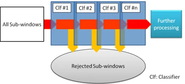
2.1 Scheme of detection cascade. Every sub-window is detected by every classifier (Clf ). If it does not conform detection rules of classifiers, it is

rejected right away and never be used again. . . 11

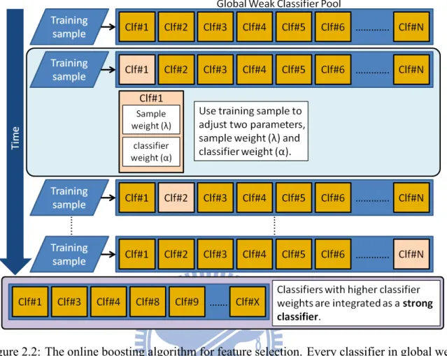
2.2 The online boosting algorithm for feature selection. Every classifier in global weak classifier pool are trained using training samples. The sample weight and classifier weights are adjusted during training. Eventually, those classifiers with higher classifier weights are selected and integrated as a strong classifier. . . 12

2.3 Tracking by classification. The object region is selected as a positive sam-ple. Neighbouring regions in search region is selected as negative samples. 13 2.4 Algorithm of online boosting for tracking. The classifier is updated every time the picture is captured and the update method is based on confi-dence map. . . 14

2.5 Example of drifting problem. From (a) to (d) are consecutive frames. From (b) to (c), the tracker drifts because the tracked lady slightly moves away from camera. . . 15

2.6 System overview of online boosting for tracking. . . 16

3.1 SemiBoost used for object tracking. Originally, semi-boost is used for machine learning via calculating similarity. The author makes use of sim-ilarity on object tracking. . . 21

3.2 Different adaptation strategies. Adopted from [17]. . . 22

3.3 Architecture of beyond semi-supervised tracking. . . 23

3.4 Tracking process of beyond semi-supervised tracking. . . 24

4.1 Truncation process of EOBT. . . 29

4.2 Truncation problem. . . 29

4.3 Tracker generation of OBT and EOBT. . . 30

4.4 The need for scalability. . . 31

4.5 Scalable adjustment using multiple scales. . . 31

4.6 Revised tracking process of EOBT. . . 32

4.7 EOBT implemented with sigmoid function. . . 33

4.8 Disappearance judgement of EOBT . . . 34

4.9 System overview of EOBT . . . 35

5.1 Wrong target problem of position error. Frame 183 in 'Coke Can' video. Adopted from [18] . . . 37

5.2 New evaluation method. . . 37

5.3 Example of ground truth construction. . . 38

5.4 Experimental video for experiment on drifting. . . 42

5.5 Experimental results on drifting. . . 43

5.6 Best case and one of worse cases of our experimental results. . . 43

5.7 Experimental video for experiment on scales. . . 44

5.8 Experimental results on scalability. (From far to near) . . . 45

5.9 Problems caused performance drops. . . 45

5.10 Best case and one of worse cases of our experimental results.(From far to near) . . . 46

5.11 Experimental results on scalability.(From near to far) . . . 46

5.12 Best case and one of worse cases of our experimental results. (From near to far) . . . 47

5.13 Experimental video for experiment on temporary occlusion. . . 48

5.15 Best case and one of worse cases of our experimental results. . . 49

6.1 Concept of manifold. Mkis a specific manifold and Ckis are submonifolds of Mk. I is some object. The distance dHis used to calculate the similarity or likelihood that object I belongs to Mk. . . 51

6.2 Integration of mentioned tracking methods . . . 52

6.3 Experimental results on drifting. . . 53

6.4 Ambiguity of each feature. . . 53

6.5 Two different appearance models.Generative model is adopted from [33]. Generative model is trained using object appearance directly. Discrim-inative model is trained using differences between objects and neigh-bouring regions. . . 54

6.6 Solve occlusion problem using MIL [18]. Because MIL is trained from the concept of bag, each part of object appearance can be recognized. This helps a lot while object is occluded. Statements below the table describe how MIL works in detail. . . 56

6.7 Experimental result on searching using particle filter. Adopted from [34]. 57 6.8 Stability on drifting. . . 57

6.9 Stability on scalability.(Forward) . . . 58

6.10 Stability on scalability.(Backward) . . . 58

6.11 Stability on temporary occlusion. . . 59

6.12 Experimental results on temporary occlusion. . . 59

A.1 AdaBoost algorithm [22]. . . 2

A.2 AdaBoost in action [22]. . . 4

A.3 Algorithm of online boosting [22] . . . 6

Chapter 1

Introduction

Visual tracking, or object tracking, has been studied for decades. The object for visual tracking is to continuously label objects of interest in video sequences. This is a prior step for further image processes. Lots of applications, like video indexing, human-computer interaction (HCI), traffic monitoring, augmented reality (AR), demand executions of visual tracking. For example, automated surveillance needs information about suspicious human motion. To acquire those information, human tracking shell be performed first, and then traces can be recorded for further analysis.

In this chapter, challenges and issues of visual tracking are discussed first. Recent devel-opments of object tracking come after. Contributions and synopsis of this paper are mentioned at the end of this chapter.

1.1

Challenges

Tracking is continuously finding region of interest (ROI) in frame sequences. The most intuitive tracking method is recording every pixel value of ROI at first frame. Then, tracking is implemented as finding the most similar region as records in the succeeding frames. However, in frame sequences, there are lots of variations need to be took into consideration. For example, illumination, shape variations or occlusions. These variations make object tracking more diffi-cult than imagination. Here, several challenges are summarized as follows [1].

Loss of Information

Images are formulated by projecting 3D real world on 2D sensors. Useful information like spatial structures has been destroyed.

Noise

Noises occur from different sources, from hardware to software. From signal processing viewpoint, when and where noises occur are unpredictable. To design a noise-sustained system is challenging.

Complex Object Motion

Object motions vary diversely. Thought kinematics theorems can be used, object motion in 3D environment is hard to predict. Some researchers have made use of this prediction as context information [2]. Using this method, the false positive rate of tracking accuracy decreases to an extent. However, computational cost should pay at the same time.

Object Body

Object could be coarsely categorized in rigid, non-rigid or articulated body. Their prop-erties are different from objects to objects, and the borderlines between them are vague. Especially, articulating object has been independently addressed in recent research [3].

Occlusions

Due to loss of 3D information, partial or entire occlusions come up frequently. Recently, some researchers use adaptive appearance models as a tracking method. Adaptive ap-pearance model continuously learn new apap-pearances, which has the ability to conquer variations like illumination. Nevertheless, when occlusions happen, adaptive methods learn wrong appearances. This problem is coined as template update problem, or drifting, which is addressed in the rest of this thesis.

Complex Object Shapes

Object shapes cause problems. At first look, complex object shapes are hard to describe. Usually, primitive geometry shapes are used to stand for objects, but in the meantime, background is introduced. The drifting problem mentioned earlier also occurs in this sit-uation.

Scene Illumination Changes

Illumination changes cause problems since object appearance learnt from previous frame is different from now. Previous object appearance can not be completely trusted. Several tracking methods have been proposed to solve this problem.

Processing Time Requirements

Though usually real-time, 20 frames per second (fps), is demanded, different situations change this requirement. For example, in normal video surveillances, 7 fps is fast enough, which eases time requirement. Trade-off between accuracy and processing time should be taken into account.

1.2

Issues of Existing Tracking Methods

Challenges of visual tracking have been discussed in previous section. This section focuses on issues of tracking methods. Each method has its applicability. For example, Kanade-Lucas-Tomasi (KLT) tracker [4] is properly used in augmented reality (AR) field, because object mo-tions could be detected precisely. However, for a 24 hour surveillance system, illumination variation is one of main concerns. Cannons [5] and Yilmaz [1] have discussed different track-ing methods ustrack-ing their own taxonomy. Here these methods are classified in functional aspects. First, the ways these methods represent ROI are described, with or without a priori model. Also,

their pros and cons are mentioned. Finally, comparisons on tracking methods and summary are at the end of this section.

1.2.1

Object Representations

First of all, object representations are tightly related to tracking methods and their applica-tions. Once an object representation is adopted, the applicability has also been fixed. Yilmaz [1] has made an extensive survey on his paper. However, for clarity, we adopt Cannons' catego-rization [5]. He classifies these object representations into three main categories, points, edges and lines, and regions. These categories are introduced respectively as follows.

Points

Points has been an excellent object representation since Harris interest point detector was proposed [6]. Nowadays, local invariant point feature, like SIFT [7] and SURF [8] ,has gained lots of attention. Point representation is popularly used in Augmented Reality and other applications, because it possesses object orientations and can be computed very fast. Point representation is a simple method to represent objects. However, due to this simpli-fied representation, lots of objects would have similar representations. In this situation, tracker might get confused and the odd of false positive is elevated. In reality, point repre-sentation does not precisely learn objects. All information they held are points. Tougher jobs like object recognition, point representation seems not applicable to.

Edges and Lines

Edge features are used in many tracking systems. An edge is defined as pixels lie on the boundary between regions. Usually edges are grouped into lines, and an easy detection using filter banks can be applied. Cannon has addressed three categories of line detectors,

monly used method is the famous Hough transform. In fact, due to discard too much potential information, tracking using edges or lines is getting less attention.

Regions

Recently, using regional features for tracking becomes popular. There are two types of regional descriptors, color histograms and histograms of gradients. Color histogram meth-ods are invariant to translation and rotation. However, the spatial information collapses at the same time. Also, depending on color, illumination variations severely damage color histogram. On the other hand, histogram of gradients (HOGs) is robust to illumination variations, but easily affected by cluttered background. Therefore, hybrid methods have also been addressed. Because regional features have better ability to describe objects, they are extensively used in object tracking.

1.2.2

Object Models

Object models help tracking in that shape variations are handled. Using object models, object shape in three dimension space is revealed and predictable. In this way, more information can be gathered using kinematics. However, model construction is the bottleneck. If every object model is constructed before tracking, applicability is consequently reduced. In practical applications, human tracking with models is the most common usage, like Microsoft⃝XBOXR

360. It is a trade off between tracking accuracy and applicability.

1.2.3

Tracking Methods

In Cannon's survey [5], four categories of tracking methods are classified. They are ing using discrete features, tracking with contours, region-based trackers and combined

track-Tracking with contours use methods like Snake [9] or level sets [10]. Region-based trackers and combined trackers are recently become popular. In region-based trackers, Cannon has addressed blob trackers, pixel-wise template tracking, kernel histogram methods. These methods usually use statistical methods to track. On combined trackers, methods of integrating above-mentioned designs are discussed. Though tracking methods possess respective merits, drawbacks are ac-companied with them. It is easy to see that, recent development walks towards methods using higher dimensions to describe objects.

1.2.4

Motion Estimation

Some tracking methods use motion models to make searching efficient. Thanks to New-tonian mechanics, object motion is predictable. Nevertheless, in practical situations, noises damage object motion estimation. Once observation made in previous frame was mixed with noises, estimation is then deviated. Finally, error accumulation breaks the system. Correct mo-tion estimamo-tion helps object tracking in computamo-tion reducmo-tion, but it also increases the risk of false positive.

Several object tracking approaches have been addressed from object representations to tracking methods. Different approaches are suitable for different applications. In next section, developments of tracking methods are discussed.

1.3

Developments of Tracking Methods

Yang [11] has mentioned that conventional tracking methods use prediction and verification. At previous frame, frame t− 1, tracker makes predictions for next state. Sampling and particle filtering are available prediction methods. At frame t, verification of previous predictions is

realized by observations. The overall architecture is just like recursive process of Kalman filter, prediction and correction [12]. Most of these methods require offline training and do not have high-level notion of objects. Also, they possess the same appearance model throughout frame sequences.

Recently, tracking algorithms are trying to break the limitation of using constant appear-ance model. Continuously learning and updating appearappear-ance model have made trackers endure large illumination and pose variation. In this way, tracking methods become more robust to en-vironmental variation. Yang [11] has pointed out that several tracking algorithms have applied this concept, including generative or discriminative algorithm, multiple instance learning and articulating object tracking. In this thesis, we describe some of them in related works.

1.4

Contribution

In this paper, we propose an enhanced tracking method called EOBT, which is based on Online Boosting for Tracking (OBT) [13][14]. OBT is an amazing tracking method which has ability to adapt those variations between frames. It is also a model-less tracking methods without motion estimation. However, the most crucial problem is also due to its excellent adaptability, which is called the template update problem, or drifting. This is a stability-plasticity dilemma and has been addressed in [15]. In short, increasing adaptive might causes stability drop. We import depth information to enhance OBT on drifting-resistance ability. Also, we introduce scalability for EOBT, hoping to reduce background noises caused by distance variations. To solve temporary occlusion problem, we design a new mechanism called lifetimer for our tracker. With lifetimer, tracker is able to stop updating when getting lost. Meanwhile, it differentiates temporary occlusion from disappearance. This is important for practical usage to notify system

1.5

Synopsis

The remaining part of this paper is organized as follows. Chapter 2 introduces OBT in details. Related works designed to solve drifting problem are described in chapter 3, including online semi-supervised boosting for tracking [16], beyond semi-supervised tracking [17] and tracking with online multiple instance learning [18]. In chapter 4 and 5, we propose our enhanced tracking method and demonstrate some experiments. Chapter 6 discusses and compares our methods with those in related works. Finally, conclusion summarizes our research in chapter 7. More information about boosting, online boosting, semi-supervised learning and multiple instance learning are attached in appendices.

Chapter 2

Background

In this chapter, the tracking method, OBT, is described in detail. It has been used in related works and proposed method. The reason why the online boosting algorithm is adopted in pro-posed method is mentioned first. Then, the online boosting algorithm used for feature selection and object tracking comes after. For more information about the boosting and online boosting algorithm, please refer to appendices.

2.1

Preliminary

Boosting is an ensemble learning algorithm used to distinguish one category from another. It has been researched theoretically and experimentally for past two decades [19] [20]. Research shows that, boosting can be interpreted as additive logistic regression [20], which means that the loss function of boosting is an exponential function and boosting can be regarded as a greedy learning method. Also, in the boosting algorithm, margins between categories keep increasing during consecutive iterations even when classification is finished. These two merits have made boosting widely applied into diverse research areas. For example, Viola and Jones [21] apply boosting algorithm to face detection and achieve remarkable success.

Originally, the boosting algorithm ,also known as batch boosting, uses all training samples in one iteration. To increasing its applicability, the batch boosting algorithm has been further developed in an online manner, called online boosting. In the online boosting algorithm, a train-ing sample is only used once and discarded forever. In this manner, online boosttrain-ing algorithm

is appropriate for real-time applications. However, the major challenge is that, the hypothe-ses returned from online boosting algorithm may not be identical to those returned from batch boosting algorithm.

To solve this inconsistency, Oza [22] modifies the weight adjustment scheme in batch boost-ing algorithm and proves that usboost-ing lossless learnboost-ing algorithm as base model, the hypotheses returned from online boosting would converge to those returned from batch boosting. Lossless learning algorithms are described in appendices. Concerning about theories of convergence, please refer to Oza's PhD thesis [22]. With Oza's achievement, Grabner and Bischof [13] lever-age the online boosting algorithm for feature selection and object tracking, as described in 2.2 and 2.3.

2.2

Online Boosting for Feature Selection

In 2006, Grabner and Bischof have pointed out that, in the online boosting algorithm, the importance adjustment of samples is modified. Single sample is propagated through all base models. This modification solved the crucial problem of unknown weight distributions of en-tire training samples. Therefore, Grabner and Bischof applied online boosting algorithm and proposed a novel feature selection method.

Grabner et al. [14] [13] have introduced selectors into their algorithm. The selector selects the best weak classifier from global weak classifier pool [14]. In [13], several local weak classi-fier pools are used for determining a selector, while the local weak classiclassi-fier pools are replaced with one global weak classifier pool in [14] for better performance. Please refer to the illustra-tion shown in Figure 2.2. We consider that, the mechanism provided by selectors is similar to cascade structure designed by Viola and Jones [21]. See Figure 2.1.

Figure 2.1: Scheme of detection cascade. Every sub-window is detected by every classifier (Clf). If it does not conform detection rules of classifiers, it is rejected right away and never be used again.

The importance of sample (λ) is initialized to 1. When one sample enters, all weak classifiers are used to judge this sample. After judgement, errors of weak classifiers (e1, e2... en) are

evaluated. The weak classifier with the lowest error is selected as the first selector. Then, the voting weight (αi, where i is the index of the selector) of the selector is calculated according to

its error and can be represented as

αi = 1 2 × ln( 1− ei ei ). (2.1)

Next, the importance of the sample is adjusted for the next selector (see the following equa-tions) according to the error ei−1of the previous selector.

if the judgement of previous selector is correct,

λ = λ× 1 2× (1 − ei) (2.2) else λ = λ× 1 2× (ei) (2.3) end if

After calculating its voting weight and adjusting importance, the sample with the adjusted importance is propagated to the next selector. When completing selecting weak classifiers for

Figure 2.2: The online boosting algorithm for feature selection. Every classifier in global weak classifier pool are trained using training samples. The sample weight and classifier weights are adjusted during training. Eventually, those classifiers with higher classifier weights are selected and integrated as a strong classifier.

all selectors, these selectors (hsel

i ) are then merged to form a strong classifier (hstrong).

hstrong = sign(

N

∑

i=1

αi× hseli (x)), (2.4)

where αi is the voting weight of the ith selector, and sign function is defined as

sign(x) =                    −1, if x < 0, 0, if x = 0, 1, if x > 0. (2.5)

2.3

Online Boosting for Tracking

To make use of online boosting for object tracking, Grabner et al. have designed a new procedure. There are two stages in this procedure, training stage and tracking stage. We illustrate them separately as follows.

2.3.1

Training Stage

Figure 2.3: Tracking by classification. The object region is selected as a positive sample. Neigh-bouring regions in search region is selected as negative samples.

The goal for training stage is to build a tracker for tracking. To answer the needs of object tracking, Grabner et al. [13] use the tracked object as a positive sample and surrounding back-ground as negative samples. See Figure 2.3. They only use first frame for training because the ROI is decided by user and can be fully trusted. Since online boosting is a kind of supervised learning, the first frame is regarded as his teacher for tracking on next frame. After using online boosting for feature selection, a strong classifier distinguishes tracked object from background is made. This strong classifier could be regarded as a tracker for further usage.

2.3.2

Tracking Stage

After constructing the strong classifier for tracked object, first frame is then discarded. On next frame, search region is specified according to the previous tracked object position. See Figure 2.4 for better illustration. The tracker created by previous frame is used scanning every position in the search region. While scanning, the tracker evaluates every position and produce hypotheses. These hypotheses estimate in what degree of confidence that the corresponding position is the tracked object. In other words, hypothesis is a kind of similarity estimation. A confidence map is created after scanning, see right image on second row of Figure 2.4. The position with highest confidence is chosen as new object position. This procedure is iteratively

Figure 2.4: Algorithm of online boosting for tracking. The classifier is updated every time the picture is captured and the update method is based on confidence map.

(a) frame #199 (b) frame #200 (c) frame #201 (d) frame #202 Figure 2.5: Example of drifting problem. From (a) to (d) are consecutive frames. From (b) to (c), the tracker drifts because the tracked lady slightly moves away from camera.

applied to every consecutive frame. Hence, object tracking could be achieved.

Before tracking on next frame, the tracker should be updated according to new object po-sition. This step makes tracker has adaptability to adapt variations. Another thought is that, in training stage, a tracker is made by constructing an internal appearance model. The tracker uses this internal appearance model to match with new coming frames. Since online boosting for tracking is a supervised learning process, the tracker should trust new object position deter-mined by itself. New object position is regarded as a new teacher and used to update tracker's internal appearance model. This step is also the reason why drifting problem occurred. Because position estimation is not always correct, slight errors come in. These slight errors are learnt by tracker. Hence, errors are accumulated during object tracking, causing tracker lost or to be mistrusted. See Figure 2.5.

For better illustration of online boosting for tracking, we put a system overview in Fig-ure. 2.6. Two stages form the system, training stage and tracking stage. In training stage, first gray image is used to generate a tracker. This tracker is then used to track on the first image several times for training. Number of training iteration can be set by user. In tracking stage, the trained tracker is used on succeeding frame sequence. Similar process is carried out on all frame sequence. If confidence of tracker is under 0, that means the tracker is lost. The tracking process exit if tracker lost or all frames are been tracked.

Figure 2.6: System overview of online boosting for tracking.

2.4

Summary

In summary, online boosting for tracking is a two-stage tracking method. First, internal template is constructed in training stage. Online boosting for feature selection is used to train the tracker. Next, in tracking stage, the tracker is used to search new object position by selecting the position with best confidence. Then tracker fully trusts this new object position and update internal appearance model according to it. This self learning is classified as supervised learning strategy. One of the key problems of this strategy is error accumulation. In object tracking applications, error accumulation causes drifting. In next chapter, several researches on drifting are stated in company with pros and cons. Different learning strategies are also been used to suppress drifting.

Chapter 3

Related Work

In this chapter, three drifting-suppressing methods are introduced. Our scope is limited in model-less tracking methods without motion estimation, and including appearance updating skills. Specifically, we adopt discriminative tracking methods, not generative ones. For gener-ative tracking methods, please refer to [23] or [24]. Here in this chapter, we introduce online semi-supervised boosting for tracking [16], beyond semi-supervised tracking [17], and tracking with online multiple instance learning [18] as follows.

3.1

Online Semi-Supervised Boosting for Tracking (OSSB)

Semi-supervised learning is a learning strategy exploiting not only known data, but also un-known data for learning. Recently semi-supervised learning has gained a lot of attention because known data collection is always a tedious work. For tracking applications like human tracking for example, labelling people in every frame is an inevitable preprocessing work. To exploit known data, researchers have proposed many methods to bridge the gap between known and unknown data. Xiaojin has maintained a comprehensive survey about semi-supervised learning on his website1 _{[25]. Since Mallapragada's version [26] of semi-supervised learning has been}

adopted by Grabner [16], we illustrate Mallapragada's theory in appendices. Here we only in-troduce how Grabner et al. [16] make use of their semi-supervised learning strategy on object tracking.

The key problem Grabner et al. solved is drifting problem. Grabner believes that,

mulating the update process in a semi-supervised fashion could significantly alleviate drifting problem [16]. They combine decision of a given prior classifier, HP_{(x), and an online classifier,}

Hn(x), to estimate object position. On the first frame, the prior classifier is trained using method

of original OBT. This prior classifier can be regarded as the teacher in all tracking process. Other frames are belongs to unknown data, which needs to be classified using semi-supervised learn-ing. Formally, the Mallapragada's deduction on SemiBoost told us that the best weak classifier could be obtained using

hn= arg min hn ( 1 |χL| ∑ x∈χL hn(x)̸=y ωn(x, y)− 1 |χU| ∑ x∈χU (pn(x)− qn(x))αnhn(x) ) , (3.1) where pn(x) = e−2Hn−1(x) 1 |χL| ∑ xi∈χ+ S(x, xi) + 1 |χU| ∑ xi∈χU S(x, xi)eHn−1(xi)−Hn−1(x), (3.2) qn(x) = e2Hn−1(x) 1 |χL| ∑ xi∈χ− S(x, xi) + 1 |χU| ∑ xi∈χU S(x, xi)eHn−1(x)−Hn−1(xi), (3.3) and ωn(x, y) = e−2yHn−1(x). (3.4)

The weight αn can be obtained by taking derivative of Eq.3.1 with respect to αnand setting it

to zero [27], where αn = 1 4ln ( 1 |χU| (_∑ x∈χU hn(x)=1 pn(x) + ∑ x∈χU hn(x)=−1 qn(x) ) + 1 |χL| ∑ x∈χL hn(x)=y ωn(x, y) 1 |χU| (_∑ x∈χU hn(x)=1 qn(x) + ∑ x∈χU hn(x)=−1 pn(x) ) + 1 |χL| ∑ x∈χL hn(x)̸=y ωn(x, y) ) . (3.5)

For positive samples, ∑_x

i∈χ+H

sim_{(x, x}

i) is a probability measure that x corresponds to the

positive class. We could express as ∑ xi∈χ+ Hsim(x, xi)≈ H+(x), (3.7) also, ∑ xi∈χ− Hsim(x, xi)≈ H−(x). (3.8)

Here, Grabner et al. use the prior classifier to measure similarity, so the probability measure of positive and negative samples is directly replaced by HP(x), i.e., H+(x) ∼ HP(x) and

H−(x)∼ 1−HP_{(x). On the other hand, since boosting could be viewed as additive logistic}

re-gression by stage wise minimization of the exponential loss L =∑_x∈χLe−yH(x)and confidence

measure is

P (y = 1|x) = e

H(x)

eH(x)_{+ e}−H(x). (3.9)

Therefore, Eq.3.2 and Eq.3.3 are simplified as

˜ pn(x)≈ e−Hn−1(x) ∑ xi∈χ+ S(x, xi)≈ e−Hn−1(x)H+(x)≈ e−Hn−1(x)_eHP_(x) eHP_(x) + e−HP_(x) (3.10) and ˜ qn(x)≈ eHn−1(x) ∑ xi∈χ− S(x, xi)≈ eHn−1(x)H−(x)≈ eHn−1(x)_e−HP(x) eHP_(x) + e−HP(x) (3.11)

Because discriminative classifier is used, the interest would be put on their difference, ˜zn(x),

which Grabner et al. named as "pseudo-soft-label."

˜ zn(x) = ˜pn(x)− ˜qn(x) = sinh(HP(x)− Hn−1) cosh(HP_(x)) = tanh(H P (x))− tanh(H_n−1(x)). (3.12)

We put the algorithm of online semi-supervised boosting for feature selection in Algorithm 1. Also, for better illustration, we adopt the SemiBoost concept from [27] in Figure.3.1.

Algorithm 1 Algorithm 1. On-line Semi-supervised Boosting for feature selection Require: training (labeled or unlabeled) example <x,y>, x∈ χ

Require: prior classifier HP (can be initialized by training on χL)

Require: strong classifier H (initialized randomly) Require: weights λc n,m, λωn,m (initialized with 1) for n = 1, 2, ..., N do if x∈ χLthen yn = y, λn= exp(−yHn−1(x)) else yn = sign(p(x)− q(x)), λn =|p(x) − q(x)| end if for m=1,2,...,M do hn,m = update(hn,m, < x, y >, λ) if hweak n,m (x) = y then λc_n,m = λc_n,m + λn else λω n,m = λωn,m + λn end if en,m = λω n,m λc n,m+λωn,m end for m+ = argminm(en,m), en = en,m+, hsel_n = h_n,m+ if en= 0oren> 1₂ then exit end if αn = 1₂ × ln{1−e_enn} end for

Using semi-supervised boosting for tracking does help alleviate drifting. However, the problem is its applicability seems also been limited. The reason is that, the prior classifier is fixed throughout the frame sequence. Each time when position estimation is needed, the prior classifier is recalled to mutually decide position. However, if a rotating object is tracked, this limited applicability breaks the tracking system. Tracker gets lost once the tracked object starts to rotate. Therefore, semi-supervised tracker gets lost in this situation. We may conclude that, when appearance of tracked object is always the same, online semi-supervised tracking method is robust. While rotating object is tracked, this tracking method might be no longer applicable.

Figure 3.1: SemiBoost used for object tracking. Originally, semi-boost is used for machine learning via calculating similarity. The author makes use of similarity on object tracking.

3.2

Beyond Semi-Supervised Tracking (BSST)

Beyond semi-supervised tracking is proposed by Stalder et al. in 2009 [17]. Basically, they focused on extending semi-supervised learning. They pointed out that OSSB has two drawbacks. We list them as follows.

• Influence of prior classifier might not be optimal, especially in the case of partial

occlu-sion.

• The prior classifier does not specialize to a specific object, i.e., it cannot recognize similar

objects.

These two problems have been properly solved by Stalder's architecture. Please refer to Fig-ure 3.2.

Figure 3.2: Different adaptation strategies. Adopted from [17].

tional supervised learning strategy is applied. The same route as its counterpart in (a) is ideal object track. However, supervised tracking is suffered from drifting problem. In (b), the tortu-ous route represents drifting situation. In (c), semi-supervised learning strategy corrects drifting by fixed prior classifier. The filled circle is regarded as prior classifier training, and the other unfilled circles are viewed as semi-supervised learning. Nevertheless, limited adaptability of fixed prior classifier hurts its plasticity. In (d), Stalder et al. have made prior classifier adaptive conservatively. Those filled circles are tracking with updating both prior classifier and online classifier. Unfilled circles are tracking with only updating online classifier.

The overall architecture could be divided into three parts, detector, recognizer and tracker, as Figure 3.3 shown. All of them are classifiers with different level of adaptability. The detector is offline trained classifier and without updating while tracking. The recognizer is a supervised online classifier with conservative updating. Here we briefly introduce overall mechanism of beyond semi-supervised tracking. During initialization, detector, recognizer and tracker are trained using first frame. During object tracking, semi-supervised tracking process is applied

Figure 3.3: Architecture of beyond semi-supervised tracking.

with recognizer and tracker, which recognizer is acted as prior classifier and tracker is as online classifier. If tracking is successful, prior and online classifier are not updated directly. They use detector to examine the same position again to verify if it is an appropriate appearance. If so, prior and online classifiers are updated. If not, only online classifier is updated. On the other hand, if tracking failed, prior and online classifier are recreated. Then, detector is used to find a potential position on the next frame. If detector found, the prior and online classifiers are reinitialized again. If not, this frame is discarded and keeps detecting until tracked object is found. We have summarized their tracking process in Figure 3.4. Please refer.

Because detector guarantees a fixed false positive and detection rate, drifting could be de-tected during tracking. We consider that, detector is as a supervisor, which suppresses drift-ing probability. However, beyond supervised trackdrift-ing has the same limitation as semi-supervised tracking. Though beyond semi-semi-supervised tracking does extend semi-semi-supervised tracking, the overall bottleneck is locked by detector. If arbitrary object tracking is asked,

con-tional object tracking, like human tracking.

3.3

Online Multiple Instance Learning (OMIL)

Multiple instance learning (MIL) has been studied for decades. MIL learns a concept from multiple instances, whereas conventional object tracking methods directly learn from instances. MIL learning strategy is fairly reasonable because it contains a certain degree of ambiguities. For example, see Figure 3.5. These labellings are part of correct tracked object, but with different level of label noises. The ambiguity causes target to drift.

The most substantial contribution is that MIL offers bag probabilities. Here, bag could be regarded as concept described before. Bag is a set of instances and defined according to its labelling as follows.

A bag is labelled positive even if only one of the instances in it falls within the concept. A bag is labelled negative only if all the instances in it are negative [28].

We describe theories of multiple instance learning in appendices. Here, we briefly illustrate how

Babenko et al. modify MIL so as to apply it on object tracking.

Babenko et al. modify MIL to online MIL (OMIL) for object tracking, which combines online boosting [22] and MIL [29]. For online boosting, since we have described some of them in Background and introduced them in detail in appendices, we solely focus on revisions they made. The authors choose MILBoost [29] as their MIL learning strategy. Deducted from MILBoost, since boosting can be viewed as an additive logistic regression, the log likelihood of bag of MILBoost is, logL =∑ i ( log p(yi|Xi) ) . (3.13)

The bag probability model they used is Noisy-OR model, which adopted from [29], is as follows.

p(yi|Xi) = 1− ∏ j ( 1− p(yi|xij) ) (3.14) where p(yi|Xi) is a bag probability, and p(yi|xij) is probability of instances.

Because the logistic regression is executed by weak classifiers, they choose weak classifiers according to loss functionJ , i.e.,

(hk, αk) = arg max

h∈H,α

J (Hk−1+ αh), (3.15)

Algorithm 2 Algorithm 2. Online Multiple Instance Learning (OMIL) Input: Dataset{Xi, yi}Ni=1, whereXi ={xi1, xi2, ...}, yi ∈ {0, 1}

Update all M weak classifiers in the pool with data{xij, yi}.

Initialize Hij = 0 for all i, j

for k = 1 to K do for m = 1 to M do pm_ij = σ(Hij + hm(xij) ) pm i = 1− Πj(1− pmij) Lm _{= Σ} i ( yilog(pmi ) + (1− yi) log(1− pmi ) ) end for m∗ = argmaxmLm hk(x)← hm∗(x) Hij = Hij + hk(x)

Output: Classifier H(x) = Σkhk(x), wherep(y|x) = σ(H(x))

end for

where Hk−1is a strong classifier made by previous (k-1) weak classifiers, andH is all possible

weak classifiers. They model instance probability using sigmoid function as

p(y|x) = σ(h(x)), (3.16) where σ(x) is a sigmoid function. The bag probability is directly adopted from Eq. 3.14 Here they have slightly modified Eq. 3.15, which absorbed scalar weight α. The overall online MIL-Boost algorithm is depicted in Algorithm 2.

OMIL algorithm also uses architecture of online boosting for feature selection. The inner for-loop evaluates on entire global weak classifier pool, which contains M weak classifiers. The

pm_ij and pm_i correspond to instance probability and bag probability. After evaluation on all weak classifiers, hk(x) picks the weak classifier with maximum loss, see Eq. 3.13. Here, hk(x) could

be viewed as a selector. The selector is combined into stage-wise strong classifier Hij. After

deciding all k selectors, the strong classifier H(x) is a linear combination of k selectors and bag probability p(y|x) is directly obtained using sigmoid function σ(x).

clas-sifier is defined as hk(x) = log [ pt(y = 1|fk(x)) pt(y = 0|fk(x)) ] , (3.17)

where pt(ft(x)|y = 1) ∼ N (µ1, σ1). Their update rules are

µ1 ← γµ1+ (1− γ) 1 n ∑ i|yi=1 fk(xi) (3.18) σ1 ← γσ1+ (1− γ) √ 1 n ∑ i|yi=1 (fk(xi)− µ1)2 (3.19)

Similar manner is applied on y = 0.

OMIL is an excellent object tracking in that, it interprets object from the notion of object. This means that it has excellent performance on temporary partial occlusion and maintain at good object position. This tracking method is especially applicable for human tracking while appearance changes, like wearing a hat, is normally happened. Another merit is that, this track-ing method seems have the ability returntrack-ing to correct position. Please refer to their website2 seeing the experimental video 'David.' Their tracker is not correctly aligned with David's face at frame #300. However, at frame #406 when David wears back his glasses, the tracker is aligned correctly again. On the other side, drifting can still be found in experimental videos, like 'Oc-cluded Face.' We consider that OMIL has turned its attention to the book at frame #670 to #720. The same stability-plasticity problem has also struck at OMIL. Especially, in 'Coke Can', OMIL has already out of focus and turned its attention to operator's hand. This problem cannot be found from the position error on error plot in [18].

In next chapter, we proposed our own tracking method with depth info. We also proposed our evaluation method to repair shortcomings of position error.

Chapter 4

Enhanced OBT

In this paper, we propose a novel method for eliminating drifting problem. Since all related works are developed from OBT, and OBT has the ability to get through manifold problem, we choose OBT as our tracking method and enhance it. We illustrate proposed method in this chapter and discuss manifold consideration in discussion. Our approach, EOBT, consists of three mechanisms, which introduces depth, multiple scales and lifetimer to OBT. We describe them separately in the following sections.

4.1

Depth

We enhance original OBT with depth info. Thanks to Microsoft⃝XBOX 360, a compactR

solution on both color and depth info can be caught simultaneously using Kinect. The origi-nal OBT does not include depth information. We introduce depth to distinguish object from background, hoping to eliminate background interference.

In addition, the precision of depth info returned from Kinect is 16 powers of 2. We have normalized to 0-255 for convenience, not only for human reading but also stable for machine processing. We called this normalized depth values as a depth image. For succeeding paragraph, we use the word, depth images, to represent depth info.

Our goal is to exploit depth info. We consider that direct acquiring image within specific depth range helps reducing the complexity of tracking environment. Hence, according to the depth of tracked object, we can take images out with the same depth and track only on these

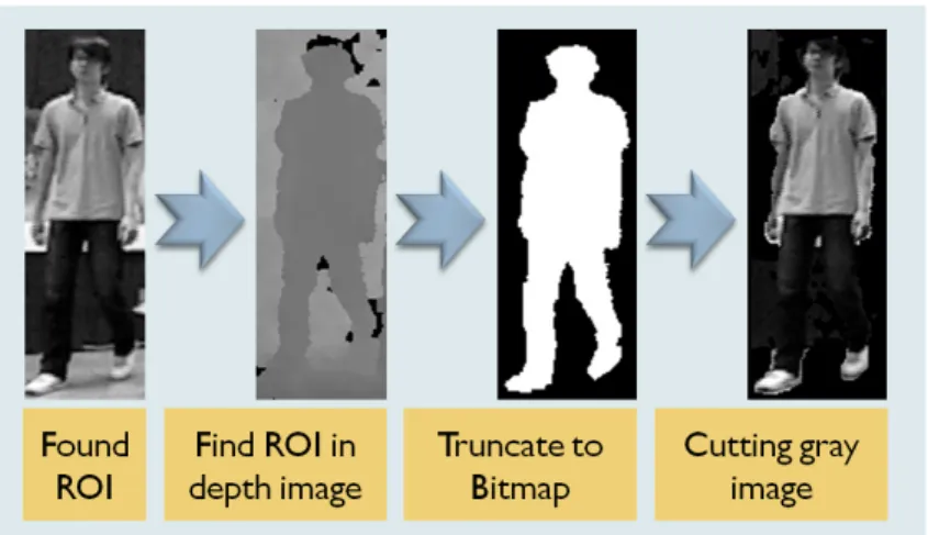
Figure 4.1: Truncation process of EOBT.

segmented images. This filtering process is illustrated in Figure 4.1.

In the beginning, tracked object, the ROI, is set by user. Next, find the same ROI on depth image. Use truncation methods to isolated tracked object from background and transform this concept into a filter. Finally, use this filter to filter out tracked object. Here, truncation method is a critical problem. Figure 4.2 illustrates this problem. In Figure4.2, the top plot is depth

Figure 4.3: Tracker generation of OBT and EOBT.

histogram of ROI. Depth range between 110 and 129 is desired truncation range. Middle image shows truncation result. Below 110 or over 129 gives bad truncation results, as shown in left and right images. There are several different truncation methods, such as fixed boundary, average value, statistics and value at middle point, etcetera. Since truncation methods could be taken as an optional choice, we let user selects his/her favour.

To show which part we revised, Figure 4.3 compares tracker generation of EOBT with OBT. EOBT has inserted object filtration to gray image. The object filtration uses the filter produced by binarizing depth image. The other parts of tracker generation remain the same. This slight revision promises that processing speed is not diminished too much.

Figure 4.4: The need for scalability.

4.2

Multiple scales

If tracker size remains unchanged, it increases probability of drifting because of too much background interferences in tracker. This problem is hard for OBT since there is no clue for distinguishing appearance changes from object distance change. See Figure 4.4. Since EOBT has exploited depth info and isolated tracked object from background, we add scalability for EOBT.

Figure 4.6: Revised tracking process of EOBT.

Normal scale adjustment is used on EOBT as Figure 4.5 shows. Multiple scales can be chosen by tracker's confidence value. The higher confidence, the more likely that guessing is correct. This is still a crucial problem since tracking accuracy is sometimes not so correct to judge object size. Once tracking accuracy is stable enough, tracker size could be stabilized. Hence, adding scalability on EOBT also exams stability and credibility of EOBT.

Since adding scalability to EOBT only revised tracking process of the overall system, we focus on this division to illustrate our revision. See Figure 4.6. Tracking process in OBT consists of four parts. First, set patch size the same as tracker size. Next, according to search region size and overlapped percentage, generate each patch one after another. These patches are selected by tracker. The one with highest confidence is object's new position. After object's new position is settled down, the tracker is then updated based on appearance of this new position. On the other hand, tracking process of EOBT modifies patch size setting and adds scale selection. In patch size generation, generate multiple scales for tracker. Each scale is evaluated and produced re-spective confidences. These confidences are used to estimate new object size in scale selection. Finally, classifier adaptation make tracker adapts to new appearance with the chosen scale.

4.3

Enhanced OBT with Lifetimer

If object is temporary occluded, conventional tracker exits and regards that tracked object is lost. However, in practical applications, there is no endless trail for real condition. Tracker has to inform succeeding processes that tracked object is lost or just temporary occluded. We consider that, the higher the number of successful tracking means the object is tracked tightly. Chances are that, abruptly zero confidence may be viewed as temporary occlusion after several successful tracking. Hence, we design a new mechanism for EOBT called lifetimer to make judgements. This mechanism is mainly designed to distinguish temporary occlusion from dis-appearance and can be implemented using different methods. Here, we use sigmoid function for example, because we should refer to the total number of its successful tracking. Sigmoid function, which is defined in Background, is rapid increasing or decreasing around the origin. This property answers our needs.

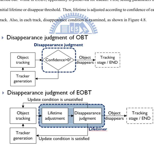
In Figure 4.7, the x-axis is tracker's lifetime. We use y-axis value to decide when disappear-ance occurred. Initial lifetime could be set any value, here we set it 0 for example. When tracking activated, every track returns a confidence value. In original design in OBT, once returned

fidence is 0, the tracker is recognized as lost. However, in our design, when confidence is more than 0, tracker's lifetime increases. When confidence is stuck at 0, tracker's lifetime starts to decrease. Also, in case that the tracker has retained successful tracking for a long time and sud-denly encountered disappearance, tracker needs to waste lots of time decreasing lifetime. The upmost value of lifetime can be set. Through lifetime design, tracker has authority to decide when to give up.

Since EOBT has only changed on disappearance judgement of OBT, we discuss those mod-ifications. See Figure 4.8. In OBT, tracking is terminated if the tracker is lost or all frames are carried out. While in EOBT, opportunity is preserved for tracker. First, setting parameters like initial lifetime or disappear threshold. Then, lifetime is adjusted according to confidence of each track. Also, in each track, disappearance condition is examined, as shown in Figure 4.8.

Figure 4.9: System overview of EOBT

To sum up, we have modified on several parts of OBT. See Figure 4.9 for better illustration. First, EOBT enhances OBT with depth image, which modifies 'Tracker generation' in system. Second, EOBT adds scalability on OBT using multiple scales, which modifies 'Tracking' part. Third, EOBT with lifetimer modifies disappearance condition to decide when should give up. These three mechanisms enhance original OBT in different parts, and the most important, we think these enhancements increase object integrity. We design three experiments to exam our proposal on next chapter. In discussion chapter, we discuss our tracking method with others and give a vivid view on object tracking.

Chapter 5

Experiments

In this chapter, we propose our evaluation method and use it to verify our proposal. First, preliminary gives an overview on evaluation method and implementation details. Next, three different experiments are carried out to test our proposal. Finally, summary is given in the last section.

5.1

Preliminary

In this section, we point out two drawbacks of conventional evaluation method and pro-pose new evaluation method. We use propro-posed evaluation to judge experimental results. Also, implementation and assumption are mentioned in this section.

5.1.1

Evaluation Method

Recently, in several conference papers and journals, position error is a popular evaluation method in object tracking. It is easy to implement, but less accuracy and credibility. Since ground truth is labelled by human, variations of human labelling inevitably exist. If the variation of examined tracking method is more than those of human labelling, it is still an applicable evaluation. However, since these days tracking accuracy is promoted to certain level, chances are that variations of human labelling may influence accuracy judgement. Another issue is that, although better accuracy is shown on position error plot, the tracker already loses its focus. For example, see Figure 5.1. Tracked object is the 'coke can' held by hand. In position error plot,

Figure 5.1: Wrong target problem of position error. Frame 183 in 'Coke Can' video. Adopted from [18]

MILTrack remains the best at frame #183. Nevertheless, the tracker has lost its focus and drifted to the wrist.

We think that tracked object pixels should be used to judge tracking results. These pixels represent area tracked object projects on to. If tracker has partially caught tracked object, it means the tracker is not lost. We illustrate this concept in Figure 5.2. There are two factors to judge tracking results. One factor is obviously, the percentage of tracked object in tracker, named RIO. This factor reflects the amount of tracked object area that tracker put attention on it. In addition, since scalable tracking method changes tracker size, percentage of tracked object in

(a) (b) (c) Figure 5.3: Example of ground truth construction.

tracker should be took into consideration. This is the purpose of our second factor, RIT. These two factors can be expressed using following equations.

RIO = Pixels of correctly tracked object

Total pixels of target object (5.1)

RIT = Pixels of correctly tracked object

Pixels of tracker area (5.2)

Proposed evaluation method may have problem on feasibility. Fortunately, thanks to the invention of Kinect, counting object total pixels becomes feasible. See Figure 5.3. Figure 5.3 (a) and 5.3(b) are images gathered by Kinect. Figure 5.3(c) is intercepted and binarized from depth image. Additional retouching is needed but not laborious. We use Figure 5.3(c) as ground truth for accuracy judgement.

5.1.2

Implementation

Here we list our experimental environment as follows.

(b) RAM: 1.96 GB

2. Images from Microsoft⃝XBOX 360 KinectR

(a) Color image: 640× 480 resolution

(b) Depth image: normalized depth values to 0-255 3. Libraries

(a) OpenNI ver. 1.1.0.41 for image capture (b) OpenCV ver. 2.1 for image processing

5.1.3

Assumption

In our experiments, since features are generated randomly, every experiment is conducted 100 times and comparison is on their average performance. Our analysis method is different from Babenko's research [18]. Their comparison is based on the same features and only learning algorithm have been changed. Since stability of tracking methods is also one of our concerns, we choose statistical analysis. In experiments, number of weak classifiers and base classifiers are fixed. We list parameters of OBT and EOBT as follows.

• Number of base classifiers: 50 • Number of weak classifiers: 250

• Four parameters for Kalman filter using Gaussian distribution: µP = 500; σP = 0.0005; µQ = 500; σQ = 0.0005.

1. Tracker generation

(a) Truncation method and its parameters

For example, if fixed boundary is used, upper bound and lower bound value should be settled.

(b) Background color

This parameter is for tracking dark objects. Using light background color for dark objects is more appropriate.

2. Object tracking

(a) Number of scales

Set for number of scales. (b) Multiplying factor

Multiplying factor of different scales according to previous tracker size. 3. Disappearance judgement

(a) Initial lifetime (b) Increment

Each time when tracking success, increase increment of lifetime. (c) Decrement

Each time when tracking lost, decrease decrement of lifetime. (d) Disappearance threshold

Threshold value for signifying tracked object disappear.

uses, µt = γµt−1+ (1− γ) 1 n ∑ i|yi=1 fk(xi) (5.3) and σt = γσt−1+ (1− γ) √ 1 n ∑ i|yi=1 ( fk(xi)− µt )2 . (5.4)

with Bayes rule to determine threshold of Haar-like features. On the other hand, OBT and EOBT use more complex updating method. State space model and Kalman filter is used. State space is,

µt = µt−1+ νt, (5.5)

σ_t2 = σ_t2₋₁+ νt. (5.6)

Parameters of Kalman filter are determined by,

Kt= Pt−1/(Pt−1+ R), (5.7) µt = Ktfj(x) + (1− Kt)µt−1, (5.8) σ_t2 = Kt ( fj(x)− µt )2 + (1− Kt)σ2_t−1, (5.9) Pt= (1− Kt)Pt−1. (5.10)

The hypothesis returned from weak classifier is defined as,

hweak_j (x) = pj × sign

(

fj(x)− ϑj

)

, (5.11)

where the threshold ϑj and parity pjare,

and,

pj = sign

(

µ+− µ−). (5.13) The µ+ _{is for positive samples and µ}−_{for negative samples.}

Totally, there are three experiments, drifting, scalability and temporary occlusion. In each experiment, OBT, OMIL and EOBT are verified. Due to limitations of OSSB and BSST, they are not examined in our experiment. However, a comprehensive description is given in next chapter.

5.2

Drifting

In this experiment, Objective is to exam that EOBT helps to eliminate drifting. The scenario of experimental video is that one person does translation and rotation in frame sequence. It contains 360 rotation and translation at the same time. If adaptability and drifting-resistance of tracking methods are insufficient, drifting may occur in frame sequences. There are some examples of experimental video in Figure 5.4. Especially, color of frontal view and rear view is different. Therefore, color histogram-based tracking method might get lost in this situation.

Experimental results are depicted in Figure 5.5. Compared with OBT, OMIL and EOBT have great performance. Especially, Object that EOBT has tracked almost maintains more than 80% and after frame #130, EOBT has better performance than OMIL. Since tracker size of

Figure 5.5: Experimental results on drifting.

all tracking methods remains the same in entire frame sequence, the tendency of RIO and RIT are similar. Difference is that, RIT curves become fluctuated. Reason of this phenomenon is caused by rotation of tracked person. Frontal view of tracked person is with the biggest area, which means more pixels are used to describe. On the other hand, lateral view is with the smallest area. Be aware that, in all of experiments, only frames have been tracked are took into consideration. Our purpose is to reveal actual tracking results. In this manner, the tracker's ability of judgements on missing condition is also correctly revealed from RIO and RIT curves.

Some results are shown in Figure 5.6. Experimental results which are lost in half of frame sequence are not took here. In best case, focus of tracker is always on the tracked person. In worse case, however, focus in only put on upper part of the tracked person.

5.3

Scalability

In this experiment, tracking verification is on scalability. This verification is divided into two parts. First, tracked person moves from far to near. Second, this experimental video is played backward, so that different object motion can be evaluated. Thus, tracking ability on scalability is examined in two manners. One is from far to near. The other is from near to far. Figure 5.13 shows some example of experimental video. In addition, because OMIL does not adapt scale variation, we only compare EOBT with OBT here.

5.3.1

Moving Forwards

Experimental results are shown in Figure 5.8. From frame #1 to #3 in RIO, a drop on performance has occurred. This is caused by severe rotation of tracked person. Also, from frame #25 to #27 in RIT, performance is decreasing because of fragmented depth information. See Figure 5.9. In entire frame sequence, performance of EOBT is better than that of OBT. Especially, RIT has revealed that, in varied tracker size, EOBT has remained stable around 0.7.

Figure 5.8: Experimental results on scalability. (From far to near)

Figure 5.9: Problems caused performance drops.

This means that tracker size adjustment catches up with moving speed of tracked object. If tracker size could not adjust in time, RIT curve becomes a descending curve. This situation is not happened to OBT since most trails of OBT is lost.

Figure 5.10 shows some of our experimental results. In best case, tracker size is catching up with tracked person. Be aware that these are consecutive frames from left to right and from first row to second row. In worse case, typical shrinking problem occurred just as tracking by Mean Shift [30]. This problem is caused by the distribution of random features. If representative features are gathered around at clothes of tracked person, smaller tracker gets higher confidence. We discuss this part in next chapter.

Figure 5.10: Best case and one of worse cases of our experimental results.(From far to near)

5.3.2

Moving Backwards

The experimental video is played backward to verify scalability of EOBT in different man-ner. Similar results are shown in Figure 5.11. Difference is that, previous mentioned descending curve has appeared here. Because of diminished area of tracked person, the part caught by OBT is decreased. If adjustment of tracker size caught up with tracked person, curves in both RIO and RIT remain horizontal. See EOBT curve in Figure 5.11. The ratio in RIO of EOBT remains between 0.8 and 0.9 from frame #2 to #25. The ratio in RIT decreases at first, but remain stable

Figure 5.12: Best case and one of worse cases of our experimental results. (From near to far)

from frame #9 to #25. Drops of EOBT in both RIO and RIT are caused by severe rotation of tracked person, which has been mentioned before.

Experimental results are shown in Figure 5.12. The best case consists of consecutive frames, but worse case is not. In best case, the tracker has caught up with tracked person. In worse case, however, adjustment of tracker size is slower than the speed of variation of tracked target.

5.4

Temporary Occlusion

The third experiment verifies tracking methods on temporary occlusion. If object is oc-cluded and tracker does not detect, the tracker then adapt on wrong target. Experimental video is designed as follows. Two people dressed clothes with similar color. They walk towards each other. The tracked person is the far one. When they pass each other, the tracked person is then severely occluded. Usually, tracker gets confused in this situation. Without any limitation, drifting occurred.