在多天線系統下使用Kalman濾波器之Tomlinson-Harashima 前置編碼設計

國 立 交 通 大 學

電子工程學系 電子研究所碩士班

碩 士 論 文

在多天線系統下使用 Kalman 濾波器之

Tomlinson-Harashima 前置編碼設計

Design of Tomlinson-Harashima Precoding in MIMO

Systems Using Kalman Filtering

研 究 生: 丁琬瑜

指導教授: 簡鳳村 博士

在多天線系統下使用 Kalman 濾波器之 Tomlinson-Harashima 前置編

碼設計

Design of Tomlinson-Harashima Precoding in MIMO Systems Using

Kalman Filtering

研 究 生: 丁琬瑜 Student: Wan-Yu Ting

指導教授: 簡鳳村 博士 Advisor: Dr. Feng-Tsun Chien

國 立 交 通 大 學

電子工程學系 電子研究所碩士班

碩 士 論 文

A Thesis

Submitted to Department of Electronics Engineering & Institute of Electronics College of Electrical and Computer Engineering

National Chiao Tung University in Partial Fulfillment of the Requirements

for the Degree of Master of Science

in

Electronics Engineering July 2011

Hsinchu, Taiwan, Republic of China

在多天線系統下使用 Kalman 濾波器之

Tomlinson-Harashima 前置編碼設計

研究生：丁琬瑜 指導教授：簡鳳村 博士

國立交通大學

電子工程學系 電子研究所碩士班

摘要

在本篇論文中， 我們研究了如何在多天線(MIMO)系統下運用 Kalman 濾 波器來對通道做追蹤估計，並且結合 Tomlinson-Harashima 前置編碼器來做通道等化 的 設 計 。 在 隨 時 間 和 距 離 變 化 而 持 續 變 動 的 多 天 線 系 統 底 下 ， 多 天 線 的 Tomlinson-Harashima 前置編碼器是一項可以用來消除不同訊號流之間的干擾的技 術，這項技術是髒紙編碼(Dirty paper coding)的延伸應用，和其他等化技術不同的地 方是，它可以在保持通道容量不變的前提下完成等化。而 Kalman 濾波器是一個運 用了隨機過程觀念所延伸出來的估計方法，和其他估計技術不同的是，它是將以前 到現在對要估計的變數所做的所有觀察集合起來當作估計的參考，而非只用要估計 的當時所觀察到的資訊來做估計，因此可以獲得較為準確的結果。在假設當中， Tomlinson-Harashima 前置編碼器必頇在傳輸端和接收端都完整的知道通道資訊的 前提下才會是完美的，而這個前提卻是不實際的假設。因此，為了更貼近現實的情 況，我們研究了在只有部分通道資訊的前提下，運用 Kalman 濾波器來估計通道並 且在把通道估計誤差也考慮進去的狀況下來做 Tomlinson-Harashima 前置編碼器的

最佳化系統設計。在模擬結果的部分，我們比較了在 TDD 的系統下本篇論文所提 出的方法和用線性最小均方差(LMMSE)估計法來結合 Tomlinson-Harashima 前置編 碼器的結果，發現使用 Kalman 濾波器的 BER 會表現得比使用線性最小均方差 (LMMSE) 估 計 法 還 要 好 ， 並 且 當 都 卜 勒 速 度 改 變 時 使 用 THP-Kalman 會 比 THP-LMMSE 還來得不易受影響。最後，我們也比較了在不同的模擬假設情形下 THP-Kalman 和 THP-LMMSE 的計算複雜度差異。

Design of Tomlinson-Harashima Precoding in

MIMO Systems Using Kalman Filtering

Student: Wan-Yu Ting Advisor: Dr. Feng-Tsun Chien

Department of Electronics Engineering

Institute of Electronics

National Chiao Tung University

Abstract

In this thesis, we study the problem of combining Kalman filter for channel tracking and Tomlinson-Harashima precoding for channel equalization in MIMO systems. The multiple-input multiple-output (MIMO) Tomlinson-Harashima precoder (THP) is a well known equalization structure for mitigating inter-stream interference in fading MIMO systems, which is the application of “dirty paper coding“ and can reserve the channel capacity. Kalman filter is an estimator based on the conception of random process, compare to other estimators, Kalman filter collects all previous channel information for estimating, yet the other estimators estimate the variables by considering the present observation. THP is optimal by assuming perfect channel state information (CSI) at both transmitter and receiver. However, this assumption is not achievable in real world. In this work, under the assumption of partial channel state information (P-CSI), we use Kalman estimation for channel tracking and combine the estimation into THP optimization which considers the channel estimation error. In simulation results, we compare the proposed approach with earlier works and can show that the performance (BER) of THP system with Kalman estimation (THP-Kalman) for channel tracking is superior to THP with linear-minimum-mean-square-error (LMMSE) estimator (THP-LMMSE) in

complexity of THP-Kalman and THP-LMMSE. By changing the Doppler rate (the parameter of mobility), THP-Kalman performs more flexible, while THP-LMMSE is sensitive to the varying rate of channel.

誌謝

這篇論文能夠順利完成，首先我要感謝我的指導教授簡鳳村老師，從我大四下 學期開始就給我許多的指導，引領我進入通訊系統的領域。因為老師的細心教導和 在專業領域的博學精深，讓我學習到不少研究上的方法和精神。而除了專業之外， 也謝謝老師在報告以及製作簡報上面教給我許多專業的技巧，讓我的研究所生涯獲 得的不只是課業上的進展，還有別的地方學習不到的表達能力訓練。 此外，感謝通訊電子與訊號處理實驗室所有的成員，包含各位師長、學長姐、 同學和學弟妹們。感謝劉藹璇學姐、李重佑學長、邱頌恩學長和張傑堯學長給予我 在研究上的指導與建議，以及怡茹、頌文、郁婷、俊言、兆軒、曉盈、威宇、卓翰、 智凱、強丹、書緯、偵源、凱翔和復凱等同學願意分享研究和生活上的心得和建議， 陪我度過這兩年的研究所生活。 最後，還要謝謝一直在背後強力支持我的父母以及願意無條件給予我幫助的哥 哥，讓我在這六年中無後顧之憂來學習和完成我想做的事，你們永遠是我精神上最 大的支柱。 在此，將此篇論文獻給所有愛我和我愛的人。 丁琬瑜 民國一○○年七月 於新竹

Contents

1 Introduction 1

1.1 Motivation . . . 1

1.2 Related Work . . . 2

1.3 Contributions of the Research . . . 4

2 Background Review 5 2.1 Introduction of Previous Equalization Strategies . . . 6

2.1.1 Linear Equalizations . . . 6

2.1.2 Nonlinear Equalizations . . . 8

2.2 Tomlinson-Harashima Precoder . . . 10

2.3 Autoregressive Model . . . 12

2.3.1 Correlated Fading Model . . . 13

2.3.2 Autoregressive Model . . . 13

3 Channel Tracking and THP Optimization with Partial CSI 17 3.1 System Model . . . 17

3.1.1 Channel model . . . 17

3.1.2 Downlink Training Channel . . . 18

3.1.3 Uplink Training Channel . . . 18

3.1.4 Downlink Data Channel . . . 20

3.2 Problem Setup . . . 22

3.3 Kalman Estimation . . . 22

3.5 Computation Complexity Comparison . . . 28 3.5.1 Computation Complexity of Kalman Filter . . . 29 3.5.2 Computation Complexity of LMMSE . . . 30

4 Simulations 32

4.1 Simulation Setup . . . 32 4.2 Numerical Results . . . 34

5 Conclusion and Future Work 38

5.1 Conclusion . . . 38 5.2 Future Work . . . 38

List of Figures

2.1 Linear Equalizer . . . 6

2.2 Linear Pre-equalizer . . . 7

2.3 SVD Equalizer . . . 7

2.4 Decision Feedback Equalizer . . . 8

2.5 Tomlinson-Harashima Precoding scheme . . . 10

2.6 QPSK diagram (4-ary constellation) with real number and imaginary num-ber axis. . . 11

2.7 Linear representation of Tomlinson-Harashima Precoding scheme . . . . 11

2.8 [1]Autocorrelation function R(k) true (Bessel) and for the AR(Q) model for Q = 1, 2 and Doppler rate fDT = 0.02. The second-order AR model autocorrelation matches the true expression for lag < 20, although only the first three terms are exactly equal. . . 14

3.1 TDD structure: Uplink(↑) and downlink(↓) for data transmission in fixed time slot, each time slot period is T and the time slot index is t. Three time slots delay is assumed. . . 18

3.2 Downlink Training channel: Q ∈ CnT×nR is the linear precoder which offers the receiver channel knowledge, and H , H[t]. . . . 19

3.3 Uplink Training channel: The uplink training channel transmit at t-th time slot, and the absolute symbol is N(t − 1) + n. . . . 19

3.4 THP model with nT transmit antennas and nRusers, each user is equipped with one antenna. . . 21

3.6 Traditional Optimization: Separate optimization of channel estimation and THP . . . 25 3.7 Non-traditional Optimization: Combine optimization of channel

estima-tion and THP . . . 26 4.1 Performances of uncoded BER versus SNR for fd=0.08. (a) Both THP

Kalman and THP LMMSE had uplink 4 time slots. (b) Both THP Kalman and THP LMMSE had uplink 5 time slots. . . 33 4.2 Performances of uncoded BER versus SNR for fd=0.08. In this case, THP

Kalman uplinks 4 slots and THP LMMSE uplinks 5 slots. . . 34 4.3 Performances of uncoded BER versus SNR for fd=0.20. (a) Both THP

Kalman and THP LMMSE had uplink 4 time slots. (b) THP Kalman uplinks 4 slots and THP LMMSE uplinks 5 slots. . . 35 4.4 Performance of uncoded BER versus normalized Doppler frequency for

Chapter 1

Introduction

1.1 Motivation

“MIMO broadcast channel” is a communication scenario with multiple cooperating trans-mitters (central base station), which can transmit a joint preprocessing of the signals, and multiple decentralized receivers (non-cooperating mobile stations), which process the re-ceived signals independently. MIMO techniques have been an important research topic due to their potential for high capacity, increased diversity and interference restrain. How-ever, the parallel transmission of independent data streams introduces severe inter-stream interference (ISI). Thus, how to deal with the ISI in the MIMO systems has been one of the most important research topics in modern communication systems.

Over the last years, many transmitter and receiver structures for mitigating interfer-ence have been proposed, achieving various levels of performance with varying complex-ities. Equalization strategies for multi-antenna and multi-user transmission are studied recently, including linear equalizations and nonlinear equalizations. Common examples for linear equalizers include linear (pre)equalizer [2] and singular-value-decomposition (SVD) based equalizer [3][22], and the most famous nonlinear equalizer is perhaps the decision-feedback equalizer (DFE) [4] [5]. The DFE is an equalization technique at the receiver side that is easy to implement, but suffers from the drawback of possible error propagations. Recently, Tomlinson-Harashima Precoder (THP) has emerged as a feasible approach to maintain the channel capacity for eliminating ISI. The concept of THP was

first introduced by Tomlinson [6] and Harashima/Miyakawa [7] for input single-output (SISO) inter-symbol-interference (ISI) systems, which can be seen as the dual to DFE, i.e., moving the detection structure (feedback part) from the receiver side to the transmitter side. While the DFE feeds back already quantized symbols, the already precoded symbols are fed back in a THP system and modulo operations are applied to constrain the precoded symbol power at the transmitter. By moving the feedback part to the transmitter side, THP can overcome the main shortcoming of DFE,i.e., error propa-gations. Furthermore, adopting THP at the transmitter can achieve better bit-error-rate (BER) than the linear equalizers and DFE, as shown in [8].

On the other hand, THP can be considered as the simplest practical approximation of the “dirty paper coding” (DPC) [9]. In the DPC-based structure, on the condition of perfect CSI at the transmitter, the optimal transmitter adapts the transmit signal to the interference rather than cancel it. It has shown that the channel capacity is not decreased by the additional interference known at the transmitter. However, in the real world, perfect CSI is not available. Numerous researches have introduced different kinds of methods to obtain the channel information, and many estimation approaches have used to calculate the channel coefficients. More details will be described in Section 1.2.

In this work, to approach the real world situation, we are interested in the Tomlinson-Harashima precoding strategies with partial channel-state-information for multi-antenna and multi-user transmission in wireless communication systems with time-varying Rayleigh channels. In most studies, the accuracy of time-varying CSI is limited by the available number of past training sequences. To improve the quality of CSI, we adopt the idea of Kalman filtering to track the time-varying channel coefficients.

1.2 Related Work

Over the past years, the application of THP had been combined into MIMO system and numerous research studies have been working on this issue. The temporal inter-symbol interference mitigation of THP is applied in the broadcast channel (i.e. point to multi-point transmission) by Ginis [10] and Yu [11]. Further, THP is applied into

multiple-input multiple-output (MIMO) systems by Fischer [12]. Also, he compares other popular equalization techniques with THP in MIMO system as in [8]. The optimization of THP in these research work are based on zero-forcing (ZF-THP) in frequency flat channels. Later, minimum mean-squared error based THP (MMSE-THP) is proposed in [13] in frequency selective channels, and optimum precoding order is combined into MMSE-THP in [14]. The maximum achievable information rate for ZF-MMSE-THP and MMSE-MMSE-THP is studied in [15]. Further, Lagunas [16] proposes a generalized structure of spatial THP which enables different transmission powers for each antenna, and the channel capacity bounds are also investigated. This achievable structure ensures that for variable power per transmitter, the precoding structure and its properties can be preserved. Also, an efficient algorithm for reducing the computational complexity of filter and precoding order based on symmetrically permuted Cholesky factorization is proposed in [17] and [18].

Most of the previous works assume that perfect CSI is given at the transmitter. How-ever, since CSI uncertainties always exist in real world systems, this assumption is not realistic. Recently, systems with mobility in wireless communications is a major issue. In spite of THP’s good performance, it is very sensitive to erroneous CSI, as the results shown in [19]. As CSI at the transmitter is never perfect, the system suffers from severe performance degradation. From the uplink in time-division-duplexing (TDD) systems or receivers’ limited feedback, partial CSI (P-CSI) is available at the transmitter. TDD refers to a transmission scheme that allows an asymmetric flow for uplink and downlink trans-mission. In a TDD system, a general carrier is shared between the uplink and downlink, the resource is being switched in time. The time variations of channel and channel esti-mation error lead to significant outdated CSI at the transmitter in both cases. Lampe [20] considers THP without exact CSI, Dietrich [19] proposes a robust optimization for ZF-THP with erroneous CSI and use MMSE-based prediction for channel parameters, and Liavas [21] optimizes THP based on partial-CSI with cooperative receivers (which we do not discuss in our work). MMSE-THP with P-CSI has combined Kalman estimation for channel tracking and particle filtering techniques are introduced in [22]. Dietrich [23] introduces a robust optimization for MMSE-THP with P-CSI which consider channel es-timation error, and a novel receiver based on CSI at the receivers is designed.

1.3 Contributions of the Research

Most of the previous works with the THP optimization methods are based on the assump-tion of perfect CSI. In this thesis, we relax the assumpassump-tion of perfect CSI and attempt to track the time-varying channel coefficients using the Kalman filtering, which we refer to as the Kalman-THP method. By using the Kalman estimator, we can recursively update and predict the channel coefficients using all the previous training sequences from the uplink transmission in the TDD mode. Comparing to the approach proposed in [23], the proposed Kalman-THP method can achieve comparable bit error rate performance with close computational complexity when the channel is highly time-varying.

Chapter 2

Background Review

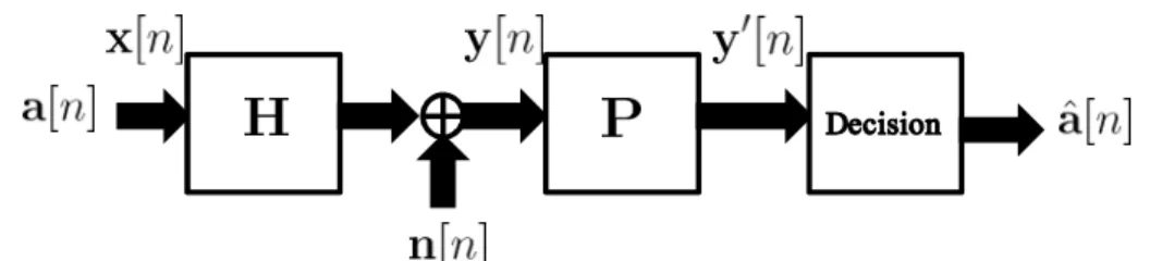
Usually, a MIMO transmission scheme is described by the basic relation y = Hx + n, where x denote the transmit vector which comprises the transmit symbols of nT parallel

data streams, and these streams are belong to different and independent users. The vectors y and n of dimension nR designate the vector of received symbols and the vector of

disturbances, respectively. The MIMO (flat-fading) channel is characterized by its nR×

nT channel matrix H.

The interference components of the transmitted vector x are present at the receiver sides. To be specific, the receive symbol of i-th antenna/user is represent as

yi = hiixi+ nT

X

j=1,j6=i

hijxj + ni (2.1)

where the second term of the equation is the i-th antenna/user’s interference from other users. Mathematically, after removing the interference, the ideal relation between the transmission scheme should be y0 _{= x + n}0_{, where y}0 _{is the equalized signal vector. The}

main goal of “equalization strategies” is to eliminate the interference terms, and numerous types of equalizers had been published in the past.

In this chapter, we will first introduce the history of equalization techniques, then we’ll focus on the details of Tomlinson-Harashima precoder. At the end of this chapter, autoregressive model will be discussed as the method of modeling the real channel.

2.1 Introduction of Previous Equalization Strategies

2.1.1 Linear Equalizations

As the name implies, “linear equalizer” is a techniques that remove the interference lin-early, some of the popular examples are linear equalizer, linear pre-equalizer and singular value decomposition equalizer. Linear equalizer implement the equalization at the re-ceiver side, on the contrary, linear pre-equalizer is proceed before the transmission, and singular value decomposition equalizer executes the equalization process jointly at trans-mitter and receiver sides. More details will be discussed as below.

Linear Equalizer

The fundamental linear equalization structure is shown in Fig. 2.1. In the figure, a[n] = [a1[n] . . . anT[n]]T is the modulated data vector, x[n] is the transmit symbol vector, and H

is the channel realization matrix, n[n] is the additive white Gaussian noise vector. In this case, a[n] = x[n]. The linear equalization strategy is to add an additional feedforward matrix P = H−1_l at the receiver, where H−1_l is the left pseudo inverse of H. Thus, the equalized signal vector is

y0[n] = H−1_l Hx[n] + H−1_l n[n] = a[n] + H−1_l n[n] (2.2) As in (2.2), the interference is eliminated. However, linear equalizer suffer from noise enhancement, i.e., H−1_l n[n], and hence, lead to poor power efficiency.

Figure 2.2: Linear Pre-equalizer

Linear Pre-equalizer [2]

The method of linear pre-equalization is the dual to linear equalizer, as in Fig. 2.2. In the condition of having the CSI at the transmitter, the data symbols are equalized prior to the transmission, i.e., P = H−1

r , where H−1r is the right pseudo inverse of H, hence, the

transmit signal vector is x[n] = Pa[n]. The received signal vector in this scheme can be written as

y[n] = HH−1

r a[n] + n[n] = a[n] + n[n] (2.3)

The linear pre-equalization scheme has overcome the disadvantage of linear equaliza-tion, nevertheless, it suffer from boosted transmit power, and also result in poor power efficiency.

Singular Value Decomposition Equalizer [3][22]

Since both linear equalization and linear pre-equalization have suffer from power effi-ciency, the SVD equalizer is presented in order to defeat the disadvantages of these pre-vious works, the block diagram is shown in Fig. 2.3. In the condition of having the CSI at the transmitter, the channel matrix can be decomposed as [24] (singular value

position)

H = UΣVH (2.4)

where U and V are unitary matrices which contain the eigenvectors of HHH _{and H}H_H,

and the diagonal terms of Σ = diag(σ1. . . σnR) are the positive square roots of the

corre-sponding eigenvalues.

By applying F = V at the transmitter and P = UH _{at the receiver, n}

R independent

and parallel sub-channels are present, and the overall signal vector y0_{[n] is}

y0_{[n] = Py[n] = Σa[n] + U}H_{n[n] (2.5)}

Since both U and V are unitary matrices, compare to linear (pre)equalization, neither an increase of the channel noise, nor of transmit power occurs. However, as the diagonal terms of Σ represent the condition of the channel, i.e., the smallest eigenvalue stand for the illest channel, the worst channel will dominate the whole BER and lead to imperfect performance, as shown in [8].

2.1.2 Nonlinear Equalizations

In this section, we will introduce one main nonlinear equalization strategies: decision-feedback equalizer, which can be seen as the predecessor of Tomlinson-Harashima pre-coder. We will briefly describe the main goal of design and compare it to linear equalizers.

Decision Feedback Equalizer [4] [5]

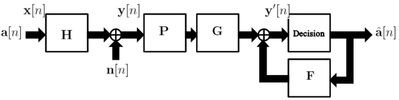
In order to improve the performance and to overcome the disadvantages at the receiver side of linear equalizations, DFE is occur, which is also called V-BLAST (Vertical-Bell Laboratories Layered Space-Time) system [25]. The block diagram of decision feedback equalizer is shown in Fig. 2.4, which is achievable if joint processing is available at the receiver sides. The main idea of DFE in MIMO is that each receiver/user can com-municate with others, and each user’s signal is decided one after another. As the second element of y0_{[n] is shift into the decision device, the first input symbol(an already decided}

symbol) is then pass through the feedback matrix F and feed back in order to subtract the interference between the first and second user. The order of making decision can provide an additional degree of freedom for minimizing the mean-square error, i.e., the symbol which transmit over the better condition channel should be decided first and so on. More details can be found in [26].

In Fig. 2.4, P is the feedforward matrix and F is the feedback matrix, G is a gain-control matrix, which is diagonal G = diag(g1. . . gnR). Note that the feedback matrix

F must be strictly lower triangular to satisfy spatial causality. The signal y0_{[n] which is}

processed at the receiver in Fig. 2.4 can be represent as

y0_{[n] = GPHa[n] + GPn[n] + Fˆa[n] (2.6)}

In DFE assumption, perf ect decision ˆa[n] = a[n] is considered. Thus, the above equation can be rewritten as

y0_{[n] = (GPH + F)a[n] + GPn[n] (2.7)}

Assume that the CSI at the receiver is perf ect, i.e., ˆH , H. Base on the equation (2.7), the feedback matrix is defined as F , I − GPH in order to remove the in-terference. For the choice of G and P, note that to preserve the noise power, i.e., E{(GPn[n])(GPn[n])H_{} = E{n[n]n}H_{[n]}, diagonal terms of G should be unit scalars,}

and P is constrain to a unitary matrix. A simple selection for G and P is applying the QR-decomposition of the channel matrix

where Q is the unitary matrix and R = [rij] is a lower triangular matrix. Thus, the scaling

matrix and the feedforward matrix read G = diag(r−1₁₁ . . . r−1

nRnR) and P = Q, and finally,

the feedback matrix is F = I − GPH = I − GR.

The DFE strategy has outperform all linear equalization scheme [8]. However, even though the performance had further improved by reordering method, the error propagation is still a main disadvantage of DFE. Also, for equalization, immediate decisions are re-quired.

2.2 Tomlinson-Harashima Precoder

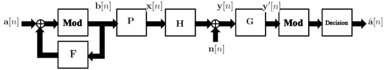
Initially, Tomlinson-Harashima Precoding [6] [7] was proposed to equalized the inter-stream-interference of severely distorting single-input single-output (SISO) channels, but in recent studies, it can be extended to MIMO channels. THP can be seen as moving the feedback part from receiver to transmitter under the condition of having CSI at the transmitter. In this case, compare to DFE, communication between different users is not needed(decentralized receivers). On the contrary, in downlink scheme, without having error propagation problem, user can still acquire other users’ information and precoded adaptively to avoid the interference by feedback matrix and feedforward matrix. Also, no immediate decisions as in DFE are required.

The THP structure is shown in Fig. 2.5, “Mod” denote the modulo operator, which is for constraining the precoded symbol power. F = [fij] is the feedback matrix and has to

be a strictly lower triangular matrix in order to maintain causality, P = [pij] is the

feed-forward matrix and G = diag(g1. . . gnR) is a diagonal scaling matrix (gain controller).

Real Axis Imaginary Axis

0

1

-1

2

-1

-2

0

1

2

Figure 2.6: QPSK diagram (4-ary constellation) with real number and imaginary number axis.

Figure 2.7: Linear representation of Tomlinson-Harashima Precoding scheme

The operation of these matrices will be described as follow. Similar in DFE, symbols are shifted into the precoding structure (modulo operator) one after another, therefore the immediate precoded symbol can have the information of all previously precoded sym-bols from feedback and thus adaptively precoded itself by feedback matrix F to avoid the interference from other users, i.e., i-th user have the information of 1-th. . .(i − 1)-th users. The remain interference can be eliminated 1)-through 1)-the feedforward matrix P. More details will be describe as follow.

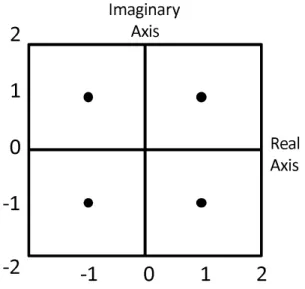
Consider that the data symbol ai[n] is modulated as M-ary constellation, i.e., for

QPSK, M=4. In the last paragraph, we interpret modulo operator as constraining the precoded symbol, this can be clearly explain by Fig. 2.6, which is a QPSK diagram (M=4). In QPSK, the data symbols a1[n] . . . anR[n] are modulated into these four points

without the modulo operator, the precoded symbol power may boost up due to the adding up feedback sequences. In order to limit the power, modulo operator is needed. Express the modulo operator mathematically, integer multiples of 2√M are added to the real and imaginary part of ai[n], the output of the modulo operator are given as

bi[n] = Mod(ai[n] − i−1 X k=1 fikbk[n]) = ai[n] + di[n] − i−1 X k=1 fikbk[n], i = 1, . . . , nR (2.8) where di[n] ∈ {2 √

M · (dI + jdQ) | dI, dQ ∈ Z} is the precoding symbols. Modulo

operator can be seen as to pull the precoded symbols back into the modulation square by adding or subtracting the real and imaginary part of integer multiples of 2√M.

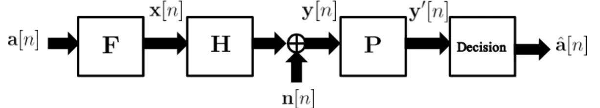
The proof in Tomlinson’s paper [6] had shown that the THP structure can be trans-formed into a linear scheme, as in Fig. 2.7. Instead of feeding the data symbols into the modulo operator and feedback, the effective data symbols v[n] = a[n] + d[n] are passed into (F + I)−1_{, where d[n] = [d}

1[n] . . . dnR[n]]T and di[n] is defined in (2.8). The signal

at the receiver is given as

y0_{[n] = GHP(F + I)}−1_{v[n] + Gn[n] (2.9)}

From the above equation, we aim to force GHP(F + I)−1 _{= I, thus the feedback matrix}

is chosen as F = GHP − I. Since G is a diagonal matrix, we can conclude that HP(F + I)−1 _{is also a diagonal matrix (for interference elimination). As the operation of F is}

to remove the previously precoded users’ interference, we can comprehend clearly that P is designed to eliminate the remain interference. Later on, the signal vector y0_{[n] =}

v[n] + Gn[n] can be restored to ˜a[n] by another modulo operator at the receiver.

2.3 Autoregressive Model

A Rayleigh characterization of the mobile radio channel follows from the Gaussian wide-sense-stationary uncorrelated scattering model, where the fading process is modeled as a complex Gaussian process. The variability of the wireless channel over time in this model is reflected in its autocorrelation function (ACF), which is depend on the propa-gation geometry, the mobile velocity and antenna characteristics. A common and simple

assumption is that the propagation path consist of two-dimensional scattering with verti-cal monopole antennas at the receivers [27]. The briefly description of this model is in next section.

2.3.1 Correlated Fading Model

For Rayleigh fading, the channel coefficient h(i,j)_{(t) is a zero-mean, wide-sense-stationary} complex Gaussian process, which is uncorrelated with h(i0_,j0₎

(t). According to Jakes’ model in [27], the channel coefficient satisfied the time-autocorrelation properties

E ½ h(i,j)_(t 1) · h(i,j)_(t 2) ¸_∗¾ ∼ J0 µ 2πf_D(i,j)T |t1 − t2| ¶ (2.10) where J0(·) is the zero order Bessel function of the first kind, T is the slot period, and

f_D(i,j)is the maximum Doppler rate from j-th transmit antenna to i-th receiver.

To simplify, we assume equal Doppler rate between all transmit-receive antenna pairs, i.e., f_D(i,j) = fD for all i ∈ {1, . . . , nR} and j ∈ {1, . . . , nT}. Thus, the corresponding

Jakes’ power spectrum density [27] (PSD) with maximum Doppler frequency fD has the

well-known U-shape bandlimit form

S(f ) =      1 πfDT 1 q 1−(_fDTf )2, |f | < fDT 0 , otherwise (2.11)

2.3.2 Autoregressive Model

In statistics and signal processing, an autoregressive (AR) model is a type of random process which is often used to model and predict various types of natural phenomena. The autoregressive model is one of a group of linear prediction formulas that attempt to predict an output of a system based on the previous outputs.

According to [28], the fading channel can be accurately modeled by a large order of autoregressive models, as in Fig. 2.8. However, large order leads to higher complexity; and further, as shown in [1], low order AR models can match the Bessel autocorrelation well for small lags k = |t1 − t2|, and can capture most of the channel dynamics, leading an efficient tracking algorithm. Thus, we use a low order AR model for channel tracking.

Figure 2.8: [1]Autocorrelation function R(k) true (Bessel) and for the AR(Q) model for Q = 1, 2 and Doppler rate fDT = 0.02. The second-order AR model autocorrelation

matches the true expression for lag < 20, although only the first three terms are exactly equal.

To approximate the time varying channel parameters h(i,j)_{(t), the following} multi-channel AR process [29] is used

h(t) = Q X q=1 A(lq)h(t − lq) + B0w(t) (2.12) where h(t) = [hT 1(t), . . . , hTnR(t)] T _{= [h}(1,1)_{(t), . . . , h}(nT,nR)(t)]T ∈ CnTnR×1, w(t) ∈

CnTnR×1 is a zero mean i.i.d circular complex Gaussian vector with correlation matrix

Rww = E{w(ti)w∗(tj)} = InTnRδij for Rayleigh variate generation, δij is the delta

function. The matrices A(lq) ∈ CnRnT×nTnR, q = 1, . . . , Q where Q is the order of

AR model, and B0 ∈ CnTnR×nTnR is diagonal due to assumption in Section 2.3.1, i.e., A(lq) = diag[a(i,j)(lq)]i,j=1i=nR,j=nT and B0 = diag[b(i,j)]i=ni,j=1R,j=nT, (i, j) is the channel path

index between different transmit-receive antenna pairs. lqdenote the number of outdated

slots and q is the index of uplink slot.

The matrix form of (2.12) can be written as

hT = AhT,pre+ Bw(t) (2.13) where hT ∈ CnRnTQ×1 hT = [h(t)T h(t − l1)T · · · h(t − lQ−1)T]T (2.14) hT,pre = [h(t − l1)T h(t − l2)T · · · h(t − lQ)T]T (2.15) and A =  A(l1) . . . A(lQ) InRnT(Q−1) 0nTnR(Q−1)×nTnR   _(2.16) B =   B0 0nTnR(Q−1)×nTnR   _(2.17)

After choosing the order Q for the AR model, we can fix A and B in (2.13), i.e.,

a(i,j)_(l

q) and b(i,j). To simplify, assume a(i,j)(lq) = a(lq) for all i ∈ {1, . . . , nR} and

j ∈ {1, . . . , nT}, i.e., all channel paths varying at the same rate. Assume that the

autocor-relation function (ACF) matrix is R. Ignoring the ill condition, assume that the inverse R−1 _{exists and the Yule-Walker equations are generated to have the unique solution of}

A [28]

where R =         r[0] r[−2] · · · r[−2Q + 2] r[2] r[0] · · · r[−2Q + 4] ... ... . .. ... r[2Q − 2] r[2Q − 4] · · · r[0]         a = ·

a(l1) a(l2) · · · a(lQ)

¸_T v = · r[l1] r[l2] · · · r[lQ] ¸_T (2.19) where r[τ ] = J0(2πfDT |τ |) is the time-autocorrelation function for given delay τ . Given

the desired ACF sequences r[τ ], the AR filter coefficients can be determined by solving the set of Q Yule-Walker equations in (2.18).

The channel varying rate is fixed via A. From equation (2.12), the power of (i, j)-th channel path can be written as

E{|h(i,j)|2} = b

(i,j)2

(1 − a(l1) − · · · − a(lQ))2

(2.20) where a(l1), . . . , a(lQ) is determined by Doppler rate as in (2.18). Thus, b(i,j)is controlled

by the channel path power. For example, a carrier frequency of 2GHz with a slot period of 0.675ms, and a normalized Doppler frequency of fDT = 0.08 corresponds to a velocity of

64km/hr. Taking order Q = 1 and lq = 2q + 1, channel power Chi = InT. Thus, this case

sets a(l1) = 0.5074 and b(i,j) ₌ √_{0.4926 for all i ∈ {1, . . . , n}

R} and j ∈ {1, . . . , nT}

Chapter 3

Channel Tracking and THP

Optimization with Partial CSI

3.1 System Model

Consider a transceiver with nT cooperative transmit antennas and nR noncooperative

re-ceivers/users, each user is equipped with one antenna. Downlink and uplink takes place in TDD mode, as shown in Fig. 3.1. Here, uplink and downlink are assumed to be recip-rocal, which means HDL = HTU L , H. Assume that data transmission is in downlink,

i.e., HDL ∈ CnR×nT, and nT antennas transmit simultaneously in one fixed time slot. As

shown in Fig. 3.1, t = t0 denote the time slot index at t0-th time slot, whereas n denote the symbol vector index transmitted in each time slot, and N is the total number of symbol vectors in each time slot, i.e., n ∈ {1, . . . , N}. Thus, the absolute symbol index is given by N(t − 1) + n.

3.1.1 Channel model

Consider a time-varying Rayleigh fading channel. Thus, downlink channel matrix H at time t is H =      hT 1(t) ... hT _(t)     =      h(1,1)_{(t) . . . h}(1,nT)(t) ... . .. ... h(nR,1)(t) . . . h(nR,nT)(t)     

, H(t) ∈ CnR×nT (3.1)

where h(i,j)_{(t) is the channel coefficient from j-th transmit antenna to i-th receiver in time} slot t. The channel coefficients are modeled as a stationary zero-mean complex Gaussian random vector with hi(t) ∼ Nc(0, Chi).

3.1.2 Downlink Training Channel

According to [23], in order to precisely design receivers, we need receivers’ channel knowledge. Thus, downlink training transmission is assumed, which are transmitted or-thogonally to the data with in the same time slot, as shown in Fig. 3.2. The receivers’ channel knowledge is determined by linear precoder Q = [q1, q2, . . . , qnR] ∈ C

nT×nR

and known training sequence b[n], and we assume each receiver has perfect channel knowledge of hT

i qi.

Q provides an additional degree of freedom in system design, the choice of qiand the

receivers’ design based on hT

i qiwill be discussed in Section 3.1.4.

3.1.3 Uplink Training Channel

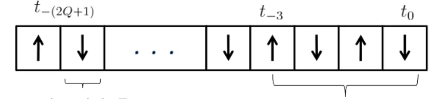
The transmitter channel state information is offered by uplink training channel, as in Fig. 3.3. Assumed that the worst time delay is three time slots. Each training se-quence s[n] ∈ CnR×1 is used to uplink at a time, and the total training sequences S

up =

[s[0] s[1] . . . s[N − 1]] ∈ CnR×N will be transmitted in every time slot, which is known

worst case delay: 3 time slots slot period = T

Figure 3.1: TDD structure: Uplink(↑) and downlink(↓) for data transmission in fixed time slot, each time slot period is T and the time slot index is t. Three time slots delay is assumed.

Figure 3.2: Downlink Training channel: Q ∈ CnT×nR is the linear precoder which offers

the receiver channel knowledge, and H , H[t].

Figure 3.3: Uplink Training channel: The uplink training channel transmit at t-th time slot, and the absolute symbol is N(t − 1) + n.

by both transmitter and receiver. Thus, the single receive signal in one time slot can be written as

yU L(N(t − 1) + n) = H(t)Ts[n] + nU P(N(t − 1) + n) ∈ CnT×1 (3.2)

where n ∈ (1, . . . , N) and the additive white complex Gaussian noise is nU P[N(t − 1) +

n] ∼ Nc(0, σn2InT).

Collecting N receive signal that transmitted in one uplink time slot, we obtain

YU L(t) = H(t)TSup+ N(t) ∈ CnT×N (3.3)

Reshape the matrix form into column form ¯ yU L(t) = vec(YU L(t)) = (STup⊗ InT)h(t) + ¯n(t) ∈ C nTN ×1 _(3.4) where h(t) , vec(H(t)T_{) = [h}T 1(t) . . . hTnR(t)] T _{∈ C}nRnT×1.

As we had discussed in Section 2.3.2, higher AR order Q offers higher precision of modeling time varying channel. Thus, we collect Q previous uplink slots into a column,

which are outdated by lq, q ∈ {1, . . . , Q}, slots. The total observation at the transmitter

can be written as

yT,pre = ShT,pre+ nT,pre ∈ CnTN Q×1 (3.5)

where hT,pre = [h(t − l1)T . . . h(t − lQ)T]T ∈ CnTnRQ×1, yT,pre = [¯y(t − l1)T . . . ¯y(t −

lQ)T]T ∈ CnTnRQ×1, nT,pre = [¯n(t − l1)T . . . ¯n(t − lQ)T]T ∈ CnTnRQ×1 and S = IQ⊗

Sup⊗ InT ∈ C

nTN Q×nTnRQ.

3.1.4 Downlink Data Channel

The downlink data channel model is shown in Fig. 3.4. The models of transmitter and receiver side are as follow:

Transmitter Model

The transmit data symbol a[n] = [a1[n] . . . anR[n]]

T _{is modulated as M-ary constellation,}

and is precoded symbol by symbol. Modulo operator ”Mod” is required in order to constrain the precoded symbol power. In Section 2.2, we had evidently explain how the modulo operator works. First, we represent the linear THP model, as shown in Fig. 3.5. The feedback matrix F = [f1. . . fnR] ∈ C

nR×nR is used to feedback the information of

previous precoded symbols, and has to be a strictly lower triangular matrix in order to ensure spatial causality. The output of the modulo operator b[n] ∈ CnR×1can be written

as bi[n] = Mod(ai[n] − i−1 X l=1 fildl[n]) = ai[n] + di[n] − i−1 X l=1 fildl[n] (3.6)

where i = 1, . . . , nR, fil is the (i, l)th element in F, and di ∈ {2

√

M · (dI + jdQ) |

dI, dQ ∈ Z} is the precoding symbols. b[n] is then pass into the feedforward matrix

P = [p1. . . pnR] ∈ C

nT×nR, the output of P reads as x[n] = P(F + I)−1v[n] ∈ CnT×1,

and the received signal at the receivers is

. . .

non-cooperative (decentralized) cooperative

Figure 3.4: THP model with nT transmit antennas and nR users, each user is equipped

with one antenna.

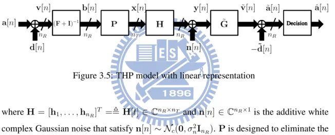
Figure 3.5: THP model with linear representation

where H = [h1, . . . , hnR]T =, H[t] ∈ CnR×nT and n[n] ∈ CnR×1 is the additive white

complex Gaussian noise that satisfy n[n] ∼ Nc(0, σn2InR). P is designed to eliminate the

interference, i.e., making the effective channel HP(F + I)−1 _{a diagonal matrix.}

Receiver Model

The (noncooperative) receivers are models as ˜G = diag[˜gi]ni=1R ∈ CnR×nR. Traditionally,

the receivers’ design is a real value scaling ˜

G = β−1_{G = β}−1_I

nR (3.8)

β is an amplitude scaling and provides the necessary degree of freedom to allow for the transmit power constraint. However, according to [23], an additional channel knowledge for the receivers can offer a degree of freedom for designing THP, as we had discussed in Section 3.1.2. By considering the correction of the channel phase, a simple and more

precise design of receivers is (As in [23]) ˜gi = β−1f (hTi qi) = β−1(h T i qi)∗ |hT i qi| (3.9) where ˜G = diag[˜gi]ni=1R, and choosing qi as the complex conjugate principal eigenvector

of the conditional correlation matrix Eh[hihHi |yT] which based on the idea of combining

(phase correction).

3.2 Problem Setup

The THP optimization is based on the MMSE criterion and the knowledge of the current channel. The total MSE of all users between v[n] and ˜v[n] in Fig. 3.5 is

MSE(P, F, β; H) = Ew,n £ kv[n] − ˜v[n]k2 2 ¤ (3.10) where v[n] = (F + I)b[n], ˜v[n] = β−1_{G(HPb[n] + n[n]), and H , H[t].}

The THP optimization problem is to design the optimum feedforward matrix P, feed-back matrix F, and receiver parameter β which can minimize the mean square error, as follow

min

P,F,βMSE(P, F, β; H)

s.t. 1) tr(PCbPH) ≤ PT

2) F : strictly lower triangular matrix (3.11) where PT is the average transmit power constraint, and Cb is the covariance matrix of vector b[n].

3.3 Kalman Estimation

Since channel matrix H is unknown, THP optimization in (3.11) can not be analyzed. Thus, we first estimate channel using Kalman estimation. The estimation is based on AR model in (2.13)

and the observation given by uplink training channel in (3.5) yT,pre = ShT,pre+ nT,pre

Where the covariance matrices of w(t) and nT,pre are Rww = δijInTnR and Rnn =

σ2

nInTnRQ. Kalman estimation can be seen as building a channel model first, and then

revise it by the channel information (uplink observation in this case) based on MMSE. Since the randomness (3.5) has introduced into the model (2.13), the equation (2.13) have to be written as

ˆ

hT = AˆhT,pre+ Kpre(yT,pre− ˆyT,pre) (3.12)

where

yT,pre− ˆyT,pre = [ShT,pre+ nT,pre] − [SˆhT,pre]

= S(hT,pre− ˆhT,pre) + nT,pre

= S˜hT,pre+ nT,pre = ˜yT,pre

˜

h can be seen as the estimation error of h. Now, we aim to find the correction item Kpre.

The error of the channel coefficients at time t (in matrix form) is ˜

hT = hT − ˆhT

= A˜hT,pre+ Bw(t) − Kpre(yT,pre− ˆyT,pre)

= (A − KpreS)˜hT,pre+ Bw(t) − KprenT,pre (3.13)

Applying equation (3.13) to the matrix form ˜ hT = (A − KpreS)˜hT,pre+ Bw(t) − h B −Kpre i w(t) nT,pre   _(3.14)

The mean-square-error of hT can be written as

MSE = E[˜hTh˜HT]

= (A − KpreS)E[˜hT,preh˜HT,pre](A − KpreS)H

h B −Kpre i Rww 0 0 R     BH −KH  

= h

InTN Q Kpre

i

APpreAH + BInTnRB −(APpreSH)

−(SPpreAH) Rnn+ SPpreSH    InTN Q KH pre   = h InTN Q Kpre i InTN Q −(APpreS H_)R−1 e,pre 0 InTN Q   ×  ∆ 0 0 Re,pre     InTN Q 0

−(APpreSH)R−1e,pre InTN Q

   InTN Q KH pre   _(3.15)

where Ppre = E[˜hth˜t], Re,pre = E[˜yT,prey˜HT,pre] = Rnn+SPpreSHand ∆ = APpreAH+

BInTnRB − (APpreSH)R−1e,pre(APpreSH)H.

By the technique of “completing the square method”, the the ideal result in equation (3.15) can be written as

MSE = ∆ + (Kpre− Kopt,pre)Re,pre(Kpre− Kopt,pre)H (3.16)

where Kopt,pre denote the optimum solution of Kpre for minimizing MSE. Comparing

equation (3.15) and (3.16), we finally get

Kpre = Kopt,pre= (APpreSH)R−1e,pre

Thus, the relation between hT and hT,prehas been solved. The recursive equations are

as follows ˆ

hT = AˆhT,pre + Kprey˜T,pre (3.17)

where

˜

yT,pre = yT,pre− SˆhT,pre

Kpre = (APpreSH)R−1e,pre

Re,pre = Rnn + SPpreSH

Pt= E{ ˜hth˜Ht } = APpreAH + BBH − KpreRe,preKHpre

where Rnnis the covariance matrix of nT,pre, Ptis the minimum value of the error

corre-lation matrix at time t where ˜ht = ht− ˆht, and ˆhT,pre is obtained by the Kalman filtering

Thus, the estimation of channel coefficients reads ˆ

ht= [[ˆhT]1· · · [ˆhT]nTnR]

T

where [ˆhT]kdenote the k-th element in vector ˆhT.

3.4 THP Optimization

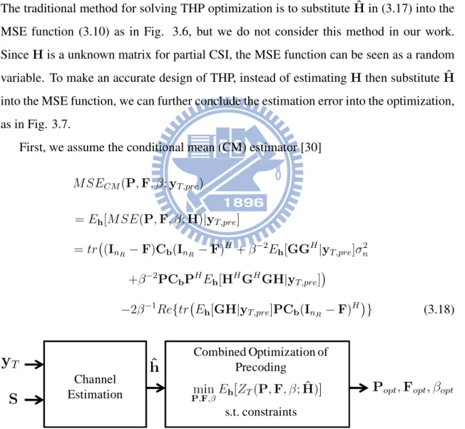
The traditional method for solving THP optimization is to substitute ˆH in (3.17) into the MSE function (3.10) as in Fig. 3.6, but we do not consider this method in our work. Since H is a unknown matrix for partial CSI, the MSE function can be seen as a random variable. To make an accurate design of THP, instead of estimating H then substitute ˆH into the MSE function, we can further conclude the estimation error into the optimization, as in Fig. 3.7.

First, we assume the conditional mean (CM) estimator [30] MSECM(P, F, β; yT,pre)

= Eh[MSE(P, F, β; H)|yT,pre]

= tr¡(InR − F)Cb(InR − F) H _{+ β}−2_E h[GGH|yT,pre]σn2 +β−2_PC bPHEh[HHGHGH|yT,pre] ¢ −2β−1_Re{tr¡_E h[GH|yT,pre]PCb(InR − F) H¢_{} (3.18)} Combined Optimization of Precoding s.t. constraints Channel Estimation

Figure 3.6: Traditional Optimization: Separate optimization of channel estimation and THP

Combined Optimization of

Channel Estimation & Precoding

s.t. constraints

Figure 3.7: Non-traditional Optimization: Combine optimization of channel estimation and THP

Thus, the new optimization problem for partial-CSI at the transmitter reads min

P,F,βMSECM(P, F, β; yT,pre)

s.t. 1) tr(PCbPH) ≤ PT

2) F : strictly lower triangular matrix (3.19) where PT is the average transmit power constraint and F is a strictly lower triangular

matrix.

The optimization problem is solved by first minimize F with fixed but unknown P, then find the solution of P and β by Lagrangian approach, as shown in [23]

pi = βP µ LyT,pre + ˆA H i Aˆi+ ˆ GNσn2 PT InT ¶₋₁ ˆ AH i ei (3.20) fi = −β−1  0i×nT ˆ Bi   pi (3.21) LyT,pre = Eh ·

(GH − Eh[GH|yT,pre])HGH − Eh[GH|yT,pre])|yT,pre

¸

= Eh[HHGHGH|yT,pre] − Eh[HHGH|yT,pre]Eh[GH|yT,pre] (3.22)

where F = [f1. . . fnR] ∈ C

nR×nR, and P = [p1. . . p

nR] ∈ C

nT×nR. Ly

T,pre is the

conditional covariance matrix of (GH)H_{, β is chosen to satisfy the transmit power}

con-straint, ˆAi denotes the first i rows and ˆBi the last nR− i rows of Eh[GH|yT,pre], ˆGN =

To calculate the CM estimate of the effective channel GH [23], we first define the complex Gaussian random variable zi = hTi qi and consider the ith row of GH. Using

the properties of the conditional expectation [31], we obtain Eh[gihi|yT,pre] = Eh · (hT i qi)∗ |hT i qi| hi|yT,pre ¸ = Eh,zi · z∗ i |zi| hi|yT,pre ¸ = Eh · z∗ i |zi|

Eh[hi|yT,pre, zi]|yT,pre

¸

(3.23) As phi|yT,pre,zi(hi|yT,pre, zi) is complex Gaussian, the CM estimator Eh[hi|yT,pre, zi]

is then [32]

Eh[hi|yT,pre, zi] = Eh[hi|yT,pre] + chizi|yT,prec

−1

zi|yT,pre(zi− Ezi[zi|yT,pre]) (3.24)

with covariances

chizi|yT,pre = Eh,zi[(hi− Eh[hi|yT,pre])(zi − Ezi[zi|yT,pre])

∗_|y T,pre] = Chi|yT,preq ∗ i czi|yT,pre = Ezi[|zi− Ezi[zi|yT,pre]| 2_|y T,pre] = qHi C∗hi|yT,preqi and µzi|yT,pre = Ezi[zi|yT,pre] = ˆh T iqi

where ˆhi is the Kalman estimator of hi.

Applying (3.24) to (3.23) yields

Eh[gihi|yT,pre] = Eh[gi|yT,pre]Eh[hi|yT,pre]

+chizi|yT,prec

−1

zi|yT,pre(Ezi[|zi||yT,pre] − Eh[gi|yT,pre]Ezi[zi|yT,pre])

with [33], the remaining terms ˆgi = Eh[gi|yT,pre] = √ π 2 |µzi|yT,pre| c1/2_zi|yT,pre µ∗ zi|yT,pre |µzi|yT,pre| 1F1 µ 1 2, 2, − |µzi|yT,pre| 2 czi|yT,pre ¶ Ezi[|zi||yT,pre] = √ π 2 c 1/2 zi|yT,pre 1F1 µ −1 2, 1, − |µzi|yT,pre|2 czi|yT,pre ¶

Summarizing the derivation, we obtain

Eh[GH|yT,pre] = ˆG ˆH + UH|yT,pre (3.25)

where ˆG = Eh[G|yT,pre] = diag[ˆgi]ni=1R and ˆH = [ˆh1, . . . , ˆhnR]T is the Kalman

estima-tion of H in (3.17).

The i-th row of UH|yT,pre is

eT_i UH|yT,pre = q

H

i C∗hi|yT,prec

−1

zi|yT(Ezi[|zi||yT,pre] − µzi|yT,preˆgi) (3.26)

where Chi|yT,pre is the covariance matrix of hi given yT,pre, and

zi = hTi qi czi|yT,pre = Ezi[|zi− Ezi[zi|yT,pre]| 2_|y T,pre] = qH i C∗hi|yT,preqi µzi|yT,pre = Ezi[zi|yT,pre] = ˆh T i qi

The solutions of THP optimization is completed.

3.5 Computation Complexity Comparison

In this section, we will analyze the computation complexity of Kalman-THP and LMMSE-THP, and then compare the differences between them. By using the same THP optimiza-tion soluoptimiza-tions, the computaoptimiza-tion complexity variaoptimiza-tion is based on the method of estimaoptimiza-tion. Thus, we will calculate the complexities of Kalman filter and LMMSE estimation only. One way to quantify this is with the notation of a f lop [24]. A flop is a floating point operation. For example, a dot product of length n involves 2n flops because there are n multiplications and n adds in either of these vector operations.

The common operations for the following calculations are matrix multiplication, ma-trix addition, Kronecker product and mama-trix pseudo inverse. For complex-number mama-trix multiplication, XY where X ∈ Cm×p_{, Y ∈ C}p×n _{involves mn(8p − 2) flops, which}

(2 × mn(p − 1) flops). To simplify the calculation, we regard the complexity as 8mnp as in [24]. For complex-number matrix addition, Z + V where Z ∈ Cm×n_{, V ∈ C}m×n

involves 2mn flops. For complex-number Kronecker product, X ⊗ Y involves 6mnp2 flops. Here, for inversion, we only consider real-number case (we only need real-number matrix inversion in the following), E−1 _{where E ∈ R}m×m _{involves (2/3)m}3 _{flops (For} more details, see [24]).

3.5.1 Computation Complexity of Kalman Filter

As we had described in Section 3.3, the solutions of Kalman filter are ˆ

hT = AˆhT,pre + Kprey˜T,pre (3.27)

˜

yT,pre = yT,pre− SˆhT,pre (3.28)

Kpre = (APpreSH)R−1e,pre (3.29)

Re,pre = Rnn + SPpreSH (3.30)

Pt= E{ ˜hth˜Ht } = APpreAH + BBH − KpreRe,preKHpre (3.31)

We first calculate the computation complexity of equation (3.31). We start with reminding the dimension of the matrices, A ∈ RnTnRQ×nTnRQ, B ∈ RnTnRQ×nTnR,

Ppre ∈ CnTnRQ×nTnRQ, Kpre ∈ CnTnRQ×nTN Q and Re,pre ∈ CnTN Q×nTN Q. Two

real-number matrices A and B are given from autoregressive model in Section 2.3.2. The elements in A are calculated from equation (2.18) where R ∈ RQ×Q _{and v ∈ R}Q×1_,

and thus involves (2/3)Q3 _{+ 2Q}2 _{flops. For matrix B, the elements b}(i,j) _{where i ∈} {1, . . . , nR} and j ∈ {1, . . . , nT} are calculated from equation (2.20), which involves

nTnR(Q + 5) flops. APpreAH involves 16(nTnRQ)3 flops, BBH involves 8(nTnR)3Q2

flops, KpreRe,preKHpre involves 8n3TnRQ3N2+ 8n3Tn2RQ3N flops and the number of flops

for addition and subtraction in (3.31) is 4(nTnRQ)2.

Next, for equation (3.30), the covariance matrix of nT,pre is Rnn ∈ CnTN Q×nTN Q,

the total training sequences in one time slot is S ∈ CnTN Q×nTnRQ and the minimum

error covariance matrix at the previous time is Ppre ∈ CnTnRQ×nTnRQ. The computation

in LMMSE calculation. The addition in (3.30) involves 2(nTNQ)2 flops and SPpreSH

involves 8n3

Tn2RQ3N + 8n3TnRQ3N2 flops.

Then, for equation (3.29), APpreSH involves 8(nTnRQ)3 + 8n3Tn2RQ3N flops, the

pseudo inverse in R−1

e,pre can also omitted since there’s a same size (nTNQ × nTNQ)

pseudo inverse in LMMSE calculation. The multiplication between (APpreSH) and

R−1

e,pre involves 8n3TnRQ3N2 flops. Similarly, 8n2TnRQN + 2nTNQ flops is needed in

equation (3.28) and 8(ntnRQ)2+ 8n2TnRQ2N + 2nTnRQ flops for equation (3.27).

Totally, the computation complexity of Kalman filter is written as

Number−of −f lopsKalman = 24(nTnRQ)3+8(nTnR)3Q2+24n3TnRQ3N2+8(nTnRQ)2

+24n3_Tn2_RQ3N + 2(nTNQ)2+ 8n2TnRQ2N + 2

3Q 3

+2nTNQ + 2nTnRQ + 2Q2+ nTnR(Q + 5) (3.32)

3.5.2 Computation Complexity of LMMSE

In this section, before we analyze the computation complexity, we first introduce the LMMSE estimation shown in [23]

ˆ h = WyT,pre (3.33) where W = ChhTS H_(SC hTS H _{+ σ}2 nInTN Q) −1 _(3.34) Ch|yT = Ch− WSC H hhT (3.35)

where Ch|yT is the covariance matrix of h given yT, ChhT = Eh[hh

H

T ] = [r[l1] . . . r[lQ]]⊗

Rh, h = vec(HT) and Ch = Eh[h(t)h(t)H], which is block diagonal assuming chan-nels from different receivers are uncorrelated, i.e., Eh[hi(t)hi0(t)H] = C_h

iδii0. The

i-th column of H(t)T _{is h}

i(t) ∼ Nc(0, Chi) as in Section 3.1.1. ChT = Eh[hTh

H T] =

CT ⊗ Ch where CT is Toeplitz with first column [r[0] r[2] . . . r[2Q − 2]]T. Since

Ch ∈ CnTnR×nTnR and CT ∈ CQ×Q, the number of flops for calculating ChhT is

2(nTnR)2Q and ChT is 2(nTnRQ)

The dimension of matrices in (3.34) are ChhT ∈ C

nTnR×nTnRQ, C

hT ∈ C

nTnR×nTnRQ

and S ∈ CnTN Q×nTnRQ. The generation of C

hhT involves 2(nTnR)

2_{Q flops and C}

hT

involves 2(nTnRQ)2 flops. The multiplication of ChhTS

H _{involves 8n}3

Tn2RQ2N flops,

SChTS

H _{involves 8n}3

TnRQ3N2+8nT3n2RQ3N flops, and the multiplication between ChhTS

H

and (SChTS

H _{+ σ}2

nInTN Q)

−1_{involves 8n}3

TnRQ3N2 flops. 2(nTQN)2 flops are included

for the addition. As in Kalman filter, pseudo inverse in (SChTS

H _{+ σ}2

nInTN Q)

−1_is

omit-ted. As the complexity of W is produced, the number of flops in equation (3.33) is 8n2

TnRQN.

Similarly, the total number of flops in equation (3.35) is 2(nTnR)2 + 8n3Tn2RQ2N +

8n3

Tn3RQ. Finally, the overall computation complexity of LMMSE reads

Number−of −f lopsLM M SE = 2(nTnR)2Q+2(nTnRQ)2+16n3Tn2RQ2N+2(nTQN)2

+8n3_TnRQ3N2+ 8nT2nRQN + 8n3TnRQ2N2

+2(nTnR)2+ 8(nTnR)3Q + 8n3Tn2RQ3N (3.36)

Since nT and nRdenote the number of transmit antennas and receivers, and Q denote

the order of AR model (which is assumed to low order in our work), these three parame-ters’ value are close. Even though the total number of training sequences in one time slot N is much larger than nT, nR and Q, we don’t see the dominant items appear in either

equation (3.32) or (3.36). The comparison is difficult by assuming variables, thus we will further compare them case by case in simulation results.

Chapter 4

Simulations

4.1 Simulation Setup

In this chapter, we consider an example with nT = 4 transmit antennas and nR = 3

re-ceivers with one antenna each, and data streams are transmitted through a Rayleigh flat fading channel. The temporal autocorrelation of the complex Gaussian channel coeffi-cients is identical for all coefficoeffi-cients, and is corresponds to Jakes’ power spectrum with maximum normalized Doppler frequency fd, i.e. Doppler frequency is normalized to the

time slot period T , fd = fD/(1/T ) where fD is the maximum Doppler frequency. System

parameters for UMTS UTRA TDD systems is taken from [34], i.e. a carrier frequency of 2 GHz and a slot period of 0.675 ms. As an example, a maximum normalized Doppler frequency fd= 0.08 corresponds to a velocity of 64 km/hr for these parameters.

Assuming an alternating uplink/downlink slots as shown in Fig. 3.1, and a worst-case delay of three time slots to the first uplink slot available with the training sequence. Thus, the observation is yT,pre = [¯y(t − 3)T, ¯y(t − 5)T . . . , ¯y(t − (2Q + 1))T]T ∈ CnTN Q×1

for Q = 5 uplink slots and sequences of length N = 32 are used for the training up-link channel. To simplify, we assume Ca = InR, Chi = InT and Cn = σn2InR where

SNR=10 log₁₀(PT/σn2) and PT = 1. For the results shown in the following figures, 300

QPSK data symbols were transmitted over 100 time slots per channel realization and av-eraged over 100 independent channel realizations, i.e., 300 symbols are totally average over 100 slots× 100 channel realizations. “THP LMMSE” is the THP optimization with

−10

0

10

20

30

10

−4

10

−3

10

−2

10

−1

SNR−BER curve of QPSK, f

d

=0.08

E

b

/N

0

(db)

BER

THP Kalman, Q=4

THP LMMSE, Q=4

THP Perfect−CSI

(a)

−10

0

10

20

30

10

−4

10

−3

10

−2

10

−1

SNR−BER curve of QPSK, f

d

=0.08

E

b

/N

0

(db)

BER

THP Kalman, Q=5

THP LMMSE, Q=5

THP Perfect−CSI

(b)

Figure 4.1: Performances of uncoded BER versus SNR for fd=0.08. (a) Both THP

−10

0

10

20

30

10

−4

10

−3

10

−2

10

−1

SNR−BER curve of QPSK, f

d

=0.08

E

b

/N

0

(db)

BER

THP Kalman, Q=4

THP LMMSE, Q=5

THP Perfect−CSI

Figure 4.2: Performances of uncoded BER versus SNR for fd=0.08. In this case, THP

Kalman uplinks 4 slots and THP LMMSE uplinks 5 slots.

LMMSE for channel estimation as in [23] and “THP Kalman” is the THP optimization with Kalman estimation for channel tracking.

By setting nT = 4, nR= 3 and N = 32, the computation complexity of THP-Kalman

and THP-LMMSE can be written as a function of Q Number − of − f lopsKalman = (5, 202, 432 +

2 3)Q

3 _{+ 72, 322Q}2_{+ 292Q + 60 (4.1)}

Number − of − f lopsLM M SE = 1, 720, 320Q3+ 1, 900, 832Q2+ 26, 400Q + 144 (4.2)

4.2 Numerical Results

Fig. 4.1(a), Fig. 4.1(b) and Fig. 4.2 show results for comparing two kinds of estimators with different number pairs of uplink slots for normalized Doppler frequency fd=0.08. In

−10

0

10

20

30

10

−4

10

−3

10

−2

10

−1

SNR−BER curve of QPSK, f

d

=0.20

E

b

/N

0

(db)

BER

THP Kalman, Q=4

THP LMMSE, Q=4

THP Perfect−CSI

(a)

−10

0

10

20

30

10

−4

10

−3

10

−2

10

−1

SNR−BER curve of QPSK, f

d

=0.20

E

b

/N

0

(db)

BER

THP Kalman, Q=4

THP LMMSE, Q=5

THP Perfect−CSI

(b)

Figure 4.3: Performances of uncoded BER versus SNR for fd=0.20. (a) Both THP

0

0.05

0.1

0.15

0.2

0.25

10

−3

10

−2

10

−1

SNR−BER curve of QPSK, SNR=20

f

d

BER

THP Kalman, Q=4

THP LMMSE, Q=4

THP Perfect−CSI

Figure 4.4: Performance of uncoded BER versus normalized Doppler frequency for SNR=20dB.

by considering Kalman estimation, on the other hand, the channel information for THP-LMMSE is only obtained by 4 presently uplink slots. The computation complexity of THP-Kalman and THP-LMMSE in this case is 334, 114, 070 flops and 140, 619, 680 flops, both of the computation complexity are in the same order, i.e.,108_{, the cost of} THP-Kalman is almost two times larger than THP-LMMSE, thus it’s a trade off between BER and complexity. In Fig. 4.1(b), the number of uplink slots for both THP-LMMSE and THP-Kalman is adding up to 5. In this case, it is not surprising that the complexity of THP-Kalman is still larger than THP-LMMSE, THP-Kalman involves 652, 113, 653 flops and THP-LMMSE involves 262, 693, 088 flops, which is still a trade off between BER and complexity. As we increase the number of uplink slots of THP-LMMSE to Q=5, as shown in Fig. 4.2, the BER shows better performance for all SNR. By comparing Fig. 4.1(a) and Fig. 4.1(b), it is clear to find out that THP-LMMSE is more sensitive to the number of uplink slots, and the BER of THP-Kalman achieves almost the same value for Q=4 and Q=5. The computation complexity of THP-Kalman and THP-LMMSE in this

case is 334, 114, 070 flops and 262, 693, 088 flops. Even though the complexity variation between THP-Kalman and THP-LMMSE are smaller, the BER of THP-Kalman still has small loss compared to THP-LMMSE. Thus, THP-Kalman is not a appropriate choice in fd= 0.08 case.

Fig. 4.3(a) and Fig. 4.3(b) show results for comparing two kinds of estimators with different number pairs of uplink slots for normalized Doppler frequency fd=0.20. In

Fig. 4.3(a), the differential value between the BER of THP-LMMSE and THP-Kalman is larger than in Fig. 4.1(a), and this shows that THP-Kalman performs the flexibility in fast fading channel. The computation complexity of THP-Kalman and THP-LMMSE in this case is 334, 114, 070 flops and 140, 619, 680 flops, both of the computation complexity are in the same order. This is still a trade off between BER and computation complexity. Fur-ther, THP-Kalman can achieve even better performance for less number of uplink slots, as shown in Fig. 4.3(b). The computation complexity of THP-Kalman and THP-LMMSE in this case is 334, 114, 070 flops and 262, 693, 088 flops, this variation is acceptable. To sum up, the proposed method is appropriate in fast fading channel(fd = 0.20) case for a

acceptable complexity.

Fig. 4.4 shows result for a fixed SNR=20dB versus normalized Doppler frequency fd.

Evidently, the performance of THP-Kalman perform better in all fdbut having more cost

Chapter 5

Conclusion and Future Work

5.1 Conclusion

We had studies Tomlinson-Harashima precoding optimization problem with partial channel-state-information under a Rayleigh flat fading channel. Kalman estimator is introduced for channel tracking and is combined into THP design. Kalman estimator is on the basis of random process, which has collect up all previous information and performs a robust estimation. Simulation results has shows better results compare to LMMSE-based THP in BER. Also, Kalman-based THP acts flexible as the Doppler frequency changes. From the view of calculating computation complexity, the Kalman-based THP achieve better BER and a close complexity in fast fading channel. With these features, the proposed Kalman-based THP is acceptable for application in the fast fading wireless broadcast channel.

5.2 Future Work

While in our work, we have proposed an effective Kalman-based THP algorithm, which decrease the BER evidently, we have not discuss about the accuracy for designing the autoregressive model, which can further improve the correctness of Kalman estimator. Also, the complexity of the THP optimization has not been analyzed.

Future works might consider the design of the AR model, i.e., in (2.13), instead of us-ing the traditional AR parameters A and B, which are chosen based on Jakes’ model. In