How Does Statutory Redemption Affect a Buyer’s Decision at the
Foreclosure Sale?
Jyh-Bang Joua*
Tan (Charlene) Leeb
Abstract
About one third of states in the U.S. offer the right of statutory redemption to a
defaulting mortgagor who can reclaim his/her foreclosed property within a certain period of
time, usually lasting for one month to one year. We derive a closed-form solution of a buyer’s
decision at the foreclosure sale, which predicts that the buyer is less likely to purchase in
states with statutory redemption than in states without it. In states with statutory redemption,
a buyer is less likely to purchase if the redemption period lasts longer or housing price
inflation fluctuates more severely because the buyer will then be hurt more by the mortgagor
who owns more valuable repurchasing option.
Keywords: American Options, Foreclosure Sale, Real Options, Statutory Redemption
a* Corresponding author. Tel.: +886-2-33663331; fax: +886-2-23679784
E-mail address: jbjou@ntu.edu.tw. Graduate Institute of National Development, National Taiwan University,
Taipei, Taiwan. b
E-mail address: tan.lee@auckland.ac.nz. Department of Accounting and Finance, The University of Auckland, Auckland, New Zealand.
2
1
1. Introduction
Foreclosure takes place when a mortgagor fails to make the required payments, and thus
defaults on a mortgage loan. In the U.S. after foreclosing a mortgage, the mortgagee may or
may not sell the collateralized property through a foreclosure sale because the mortgagor has
the equitable right of redemption, and thus can prevent the sale by paying off the outstanding
debt. Even if the foreclosure sale takes place, the mortgagor may still have a statutory right to
redeem the property by paying the price set at the foreclosure sale. About one third of states
in the U.S. provide for statutory redemption, with the period ranging from one month to one
year (Baker, Miceli, and Sirmans, 2008).
Previous work such as Clauretie (1987) argues that statutory redemption will drive down
the price for the foreclosed property because the defaulting mortgagor has the option to
reclaim it. This seems to be reasonable if a buyer attending the foreclosure sale decides
whether to purchase the foreclosed property based on the net present value (NPV) rule. As
such, the buyer is only willing to pay the property value at the date of foreclosure sale net of
the option value owned by the mortgagor. This article, which allows the buyer to postpone
the purchase by employing a real options model (Dixit and Pindyck, 1994), will investigate
two issues. The first one, which is related to the issue argued by Clauretie (1987), asks: How do statutory redemption laws affect a buyer’s incentive to purchase? The second one asks: In those states with statutory redemption, how do both the length of redemption and fluctuations
2
of housing price inflation affect a buyer’s incentive to purchase?
There are two common types of foreclosure sale, including judicial sale supervised by a
court and power-of-sale supervised usually by banks or attorney of the mortgagee. Both
usually sell a property through auctions to the buyer who bids the highest price. In this article,
we focus on interactions between a buyer and the mortgagor rather than between a buyer and
the auctioneer at a foreclosure sale. To this end, we follow the standard real options literature
to focus on a buyer who has the privileged right to purchase a foreclosed property. We
assume that the value of the foreclosed property evolves stochastically over time as a
geometric Brownian motion. We also assume that the buyer can enhance the value of the
foreclosed property, which is plausible because those who seek to make profits at the
foreclosure sale usually have more sophisticated knowledge about the real estate market than
both the mortgagor and the auctioneer. The buyer, however, will incur some unrecoverable
costs other than the purchased price.
We model the game played by the mortgagor and the buyer as a sequential one and solve
it backward. After the buyer purchases a foreclosed property, the mortgagor has the option to
choose any date during the redemption period to reclaim it at the price paid by the buyer.
When deciding whether to make an immediate purchase, the buyer will rationally anticipate
the path of the property value over the redemption period that triggers the mortgagor to
3
exercised by the mortgagor. Given this potential cost, the standard real options theory
suggests that the buyer will wait for a better state of nature to make an immediate purchase,
which in turn, reduces the probability for the mortgagor to reclaim the property during the
redemption period. Our result thus suggests that the existence of a statutory right of
redemption leads a buyer to be less likely to make an immediate purchase. This complements
that of Clauretie (1987), which argues that the existence of that right will lead a buyer to bid a
lower price, and thus the mortgage loan lender may not utilize a foreclosure in the first place.
Furthermore, we derive a closed-form solution for a buyer’s decision rule, which predicts that
in states with statutory redemption, the buyer is less likely to purchase if the redemption
period lasts longer or housing price inflation fluctuates more severely because the buyer will
then be hurt more by the mortgagor who owns more valuable option to reclaim the foreclosed
property.
Previous literature on foreclosure focuses on issues different from what we focus on. For
example, Asabere and Huffman (1992) find that the price of the foreclosed property is
determined by the same factors as the non-foreclosed property. Clauretie (1987) argues that
both the values of the mortgage and legal foreclosure costs affect the foreclosure rate.
Clauretie and Herzog (1990) investigate how state foreclosure laws affect losses of mortgage
insurers. Meador (1982) and Jaffee (1985) find that, in general mortgage loan rates were
4
Phillips and Vanderhoff (2004) find that the repeal of statutory redemption could increase the
probability of foreclosure by 20%. All the above papers do not explicitly value the option associated with the right of statutory redemption nor relate this option value to a buyer’s decision at the foreclosure sale.1
This paper is related to the literature on the pricing of American options. The mortgagor
in our framework decides the date at which to exercise an American-type call option with a
finite maturity, where the pricing formula has been provided by Barone-Adesi and Whalley
(1987), Carr (1995), and Lee and Paxson (2003).2 In addition, Jou and Lee (2009) have
applied this pricing formula to investigate how a development moratorium affects a landowner’s incentive to develop his/her vacant land.
The remaining sections are organized as follows. The second section presents the
assumptions of the model, and solve for the path of the property value over the redemption
period that triggers the mortgagor to reclaim the foreclosed property. The third section solves
for the critical level of the property value that triggers a buyer to make an immediate
purchase at the foreclosure sale. This section also investigates how various exogenous factors
affect the date at which the buyer decides to purchase and the associated gain from the
purchase. The fourth section presents the simulation analysis by employing plausible
1 Two recent papers by Miceli and Sirmans (2005) and Baker, Miceli, and Sirmans (2008) do not distinguish equitable redemption from statutory redemption. Both papers build a static model and find that an increase in the length of redemption period will reduce a mortgagor’s incentive to devote efforts to avoid default. The latter paper also investigates the issue regarding the optimal redemption period.
2 See also Geske and Johnson (1984) and Fischer (1993), both of which provide the pricing formula for the American put option with a finite maturity.
5
parameter values. The last section concludes and offers suggestions for future research.
2. Basic Assumptions
Previous literature (see, e.g., Kau, Keenan, and Smurov, 2011) has extensively
investigated the default decision made by a mortgagor. We abstract from this decision, and
instead, focus on a defaulting mortgagor whose collateralized property is subject to a judicial
foreclosure sale or power-of-sale. Suppose that the value of this property, denoted by V t( ),
evolves as: ( ) ( ) ( ) dV t dt dZ t V t , (1)
where is the expected inflation rate of the property value, is the instantaneous volatility of that inflation rate, and Z t( ) is a standard Wiener process. We assume that the
mortgagor and a buyer at the foreclosure sale are both risk-neutral and face a constant
risk-less rate, r, which is required to be greater than . As is well known in the real estate literature (see, e.g., Kau, Keenan, and Kim, 1993), the total return from holding the property
is equal to r, which is equal to , where is the convenience yield, i.e., the implicit rental rate from holding the property because the property provides housing services to the
property owner.3 We can generalize our model to the case of risk aversion in the manner of
3 As explained in Dixit and Pindyck (1994, chapter 5) the convenience yield resembles the dividend rate on a common stock, and thus will affect the buyer’s purchase timing decision. If 0, then the buyer will always hold the call option on purchasing the property to maturity. By contrast, if >0, then there is an opportunity cost to keeping the option alive, which is the housing services foregone by holding the option rather than the property. Since is proportional to the property price, the higher is the property price, the greater is the value of housing services. At some sufficiently high price, the opportunity cost of forgone housing services becomes
6
Cox and Ross (1976). Our result, however, will be the same regardless of whether we
consider a risk-neutral, or a risk-averse, environment. The buyer will never purchase the
foreclosed property unless he/she is able to operate this property better than the defaulting
mortgagor. We thus assume that after purchasing this property, the buyer can increase the property value to V t1( ), which is equal to
1
V t( ), where 0. This requirement is reasonable as professional investors have incentives to attend the foreclosure sale becausethey have accumulated sophisticated knowledge about the real estate market. They
understand that mortgagors may not take suitable care of the foreclosed properties, and thus
they can enhance the value of these properties through renovation.4 By contrast, sellers at the
foreclose sale are involuntary participants, and thus lack professional knowledge (Asabere
and Huffman, 1992). Given the relationship V t1
1
V t and the evolution of ( )V t shown by Equation (1), it follows that
1 1 ( ) 1 1 ( ) ( ) dV t dt dZ t V t , (2)where Z t is a standard Wiener process. Equation (2) indicates that the growth rate of the
value of the property in the possession of the buyer, dV t1( ) /V t1( ), has a larger drift term and a larger instantaneous volatility than their counterparts shown in Equation (1).5 Finally, we
assume that the transaction costs incurred by the buyer other than the price paid to the
great enough for the buyer to exercise the option. 4
The renovation costs can be viewed as part of the irreversible transaction costs.
5 This is supported by Reinsdorf (1994), who suggests that expected inflation usually has a positive effect on price dispersion.
7
mortgagee, denoted by K , are fully irreversible.6
3. The Repurchase and Purchase Trigger Values
As stated before, we focus on interactions between a buyer and the defaulting mortgagor
at the foreclosure sale. Thus, we assume that there is only one single buyer who can either
purchase the foreclosed property immediately or delay purchasing it. As will be shown later,
the buyer will not purchase the property until the property value reaches a threshold level. As
a result, if the threshold level is yet to come at the date when a foreclosure sale takes place,
then the auctioneer will set a new date for the foreclosure sale. This sequence will not end
until the property value evolves to the threshold level.
We model the game played by the mortgagor and the buyer as a sequential one and solve
it backward.7 Suppose that an auctioneer announces a foreclosure sale for a property at t0, and thus the value of the property is V(0). After a buyer purchases the property, the
defaulting mortgagor can reclaim it by paying the amount the property was sold for within
the statutory redemption period that lasts for T years.8 Given that the property value
6 As Brueggeman and Fisher (2006, Chapter 4) suggest, the transaction costs consist of statutory costs and third-party charges. The former includes certain charges for legal requirements that pertain to the title transfer, recording of the deed, and other fees required by state and local law. The latter includes charges for services, such as legal fees, appraisals, surveys, past inspection, and title insurance. All of these charges, however, are unrecoverable after the property is purchased.
7
The solving procedure resembles that commonly seen in the real options literature such as Jou and Lee (2007) and Wong (2006; 2009) in which the bankruptcy (or abandonment) decision is solved first, followed by the investment timing (or hedging) decision.
8 The mortgagor usually needs to pay interest as defined by statutes, in addition to the foreclosure sale price. We may allow the interest payments, which will slightly complicate our analysis a little (i.e., the number of state variables analyzed below will be two rather than one), but will yield the same qualitative result as when we abstract from them.
8
evolves stochastically, we are unable to find the exact date at which the buyer will purchase the property. Instead, the buyer’s decision rule is characterized by a critical level of V(0): If
(0)
V is greater than or equal to this critical level, then the buyer will purchase the property
immediately. Otherwise, the buyer will wait until this critical level is reached.
Let us consider a hypothetical case in which T , i.e., the defaulting mortgagor has a
perpetual right to reclaim it at any time as he wishes. We will then use the solution for this
case to derive the exercise rule for the mortgagor who has the right to reclaim the foreclosed
property only during a finite period of time.
We will solve the mortgagor’s decision rule first. Suppose that a buyer has already paid
an auctioneer V(0) to purchase a property at time t0. Thereafter, the defaulting mortgagor can reclaim the property by paying V(0) at any future date, given that the
statutory redemption period lasts forever. The mortgagor thus holds a perpetual
American-type call option, whose value is independent of the calendar date, and can thus be
denoted as F V t2( ( )). Using Ito’s lemma, we find that F V t2( ( )) satisfies the differential equation given by:
2 2 2 2 2 2 2 ( ( )) ( ( )) 1 ( ) ( ) ( ( )) 0 2 ( ) ( ) F V t F V t V t V t rF V t V t V t . (3)
Equation (3) has an intuitive interpretation: If F V t2( ( )) is an asset value, then the normal return rF V t2( ( )) must be equal to its expected capital gain given by:
9 2 2 2 2 2 2 2 ( ( ( ))) ( ( )) 1 ( ( )) ( ) ( ) ( ) 2 ( ) E dF V t F V t F V t V t V t dt V t V t . (4)
The solution to Equation (3) is given by:
1 2
2( ( )) 1 ( ) 2 ( )
F V t AV t A V t , (5) where A and 1 A2 are constants to be determined,
2 1 2 2 2 1 1 2 ( ) 1, 2 2 r and 2 2 2 2 2 1 1 2 ( ) 0. 2 2 r (6)
Suppose that V2* denotes the critical level of V t( ) that triggers the mortgagor to reclaim the foreclosed property. This critical level and the two constants, A and 1 A2, are jointly solved from the boundary conditions given by:
2 ( ) 0 lim ( ( )) 0, V t F V t (7) * * 2( 2) 2 (0), F V V V (8) and * 2 2 ( ) ( ( )) 1. ( ) V t V F V t V t (9)
Equation (7) is the limit condition, which states that the value of the mortgagor’s option to delay repurchasing becomes worthless as the property value approaches its minimum
permissible value of zero. Equation (8) is the value-matching condition, which states that, at
10
reclaim the property. Equation (9) is the smooth-pasting condition, which prevents the
mortgagor from deriving any arbitrage profits by deviating from the optimal date of
repurchasing.
Solving Equations (7) to (9) simultaneously yields:
* 1 2 1 (0) . ( 1) V V (10)
The gain for the mortgagor who makes an immediate purchase is derived by subtracting the
purchase price V(0) from V2*, thus yielding
* * 2 2 2 1 (0) ( ) (0) . ( 1) V F V V V (11)
Consequently, for the hypothetical case where the statutory redemption period lasts forever, the mortgagor will not reclaim the foreclosed property until the value of the property V t( )
reaches V2* shown by Equation (10), and will thus gain at an amount equal to F V2( 2*) shown by Equation (11).
Now consider the case in which the statutory redemption period is finite. After the buyer
purchases a property at time t0, the mortgagor has an American-type call option that expires T periods later, and can thus reclaim the property at any time during the period from 0 to T . We denote this option value as C Vm( ( ), (0), V T ), indicating that at time
the mortgagor has the option to pay V(0) to exchange for a property whose value is equal to V( ) , and if he/she does not exercise this option, he/she can still exercise it any time
11
between time and T . We follow Barone-Adesi and Whalley (1987) to price this call option. Define Vm*( ) as the critical level of V( ) that triggers the mortgagor to exercise this option at time , whose value is given by:9
* * ( )( ) * ( ) 1 1 * ( )( ) 1 ( ( ), (0), ) ( ) (0) ( ) ( ) (0) ( ( )) ( ) [1 ( )] , m m m r T r T m r T m C V V T V V e V N d e V N d T V e N d (12) where * 2 1 ( ) ln ( )( ) (0) 2 , ( ) m V T V d T 2 2 2 2 ( ) 1 1 2 ( ) 2 2 [1 r T ] r e ,
and N( ) is the cumulative standard normal distribution function.
We may use Equation (12) to numerically solve Vm*( ) . Barone-Adesi and Whalley (1987) note that an analytically tractable solution, which is approximately equal to
*
( ( ), (0), )
m m
C V V T in Equation (12), is given by:
* * * ( ) ( ) 2 1 (0) ( ( ), (0), ) ( ) (0) ( (0))(1 ) (1 ) , ( 1) h h m m m V C V V T V V V V e e ( ' 12 ) where 1 ( ) ( )( ) 2 ( ) ( 1). h r T T 9
Consider V t as an asset value. Those who purchase this asset should require compensation equal to ( ) (r ) ( )V t , given that V t is expected to grow at a rate equal to ( ) . Consequently, in Equation (12) the term
r replaces the asset yield in the formula developed in Barone-Adesi and Whalley (1987). The sum of the first two terms in the second row on the right-hand side of Equation (12) is the same as the call option pricing formula on the divided-paying stock provided by Merton (1973).
12
Solving from Equation (12') yields
*( ) ( ) (0) m V g V , (13) where ( ) 1 (1 ) ( ) 1 ( 1) h e g . (14)
Given that h( ) in Equation (14) decreases with , it follows that Vm*( ) in Equation (13) also decreases with . In other words, if less time is left for the mortgagor to decide whether to exercise the option to reclaim a property, then the mortgagor will exercise it when the
property value evolves to a lower realized value. At the end of the redemption period, time
T , the mortgagor will exercise the option as long as the realized value of the property, V T( ),
is greater than V(0), the price he/she needs to pay for regaining the ownership of the
property.
We may use Vm*( ) in Equation (13) to calculate the potential loss at the foreclosure
sale incurred by a buyer who must pay the purchase price V(0) and the transaction cost, K ,
to obtain the foreclosed property. Given that the buyer can enhance the value of the bought
property, the value of the option for the mortgagor to reclaim the property thus differs from
the loss incurred by the buyer. From the viewpoint of the buyer, at each point of time during the statutory redemption period, his/her potential loss is the value of a European call
13
the strike price, and is the expiration date. Denoting this call option value as
*
1 (0), ( ),
b m
C V V (Black and Scholes, 1973) yields
*
1
*
2 2 1 (0), ( ), r 1 (0) ( ) ( ) ( 1 ) , b m m C V V e V N d V N d (15) where
2 2 2 1 1 ln ( 1 ) ( ) 2 1 g d .Consider the decision rule for a buyer attending the foreclosure sale. Under the
assumption that the buyer is not constrained to purchase the property during any certain
period of time, the buyer thus has an option value of waiting similar to F V t2( ( )) stated before.10 Let us denote this option value of waiting as F V t1( ( )), which is given by
' '
1 2
1( ( )) 1 ( ) 2 ( )
F V t B V t B V t , where B and 1 B are constants to be determined, and 2 ' 1 and '2 are given by
' 2 1 2 2 2 2 1 1 2 ( ) >1, 2 1 2 1 (1 ) r and
' 2 2 2 2 2 2 1 1 2 ( ) 0. 2 1 2 1 (1 ) r 10 It is more plausible to allow the auctioneer to end the sequence of the foreclosure sale in a finite period of time. For example, the auctioneer can lower the reservation price each time when resetting the date for the foreclosure sale. Allowing this will complicate the analysis, but will yield the same qualitative result as disregarding this.
14
The critical level of the property value that triggers the buyer to purchase at t0, denoted by Vb*, and the two constants, B and 1 B , are solved jointly from the boundary 2
conditions given by:
1 (0)lim0 ( (0)) 0 V F V , (16)
* * * * * 1( ) 1 0 1 , ( ), T b b b b b m F V V V K
C V V d , (17) and
* * * 1 0 (0) (0) 1 (0), ( ), ( (0)) (0) (0) b b b m T V V V V C V V F V d V V
. (18)Equation (16) is the limit condition, which indicates that the buyer almost surely gains
nothing from waiting when the property value approaches its minimum permissible value of
zero. Equation (17) is the value-matching condition, which indicates that at the optimal
purchasing date, the buyer should be indifferent as to whether wait or make an immediate
purchase. The value of the former is the term on the left-hand side, while the value of the
latter is the terms on the right-hand side, i.e., the gross value from purchasing the property
*1 Vb , net of the sum of the purchase price, Vb*, the irreversible sunk cost, K , and the
potential loss resulting from the mortgagor who can exercise the repurchase option at any
time during the redemption period,
* *
0 1 , ( ),
T
b b m
C V V d
. Equation (18) is thesmooth-pasting condition, which prevents the buyer from deriving any arbitrage profits by
deviating from the optimal date of purchasing.
15 given by ' * 1 ' 1 ( 1)( ( )) b K V G T , (19) where 1
2
2
0 ( ) T r 1 ( ) ( ) 1 G T
e N d g N d d, which is requiredto be smaller than . Substituting Vb* into the right-hand side of Equation (17) yields the gain from an immediate purchase as given by:
* 1 ' 1 ( ) 1 b K F V . (20)One may argue that competitive pressure at the foreclosure sale will lead the buyer to depart
from the above decision rule.11 However, as long as the actual trigger price is equal to a
constant factor multiplied by the trigger level shown by Equation (19), then all our main
results will remain unchanged.12
Given that G T( ) shown in Equation (19) is equal to zero if T 0, and is greater than zero if T 0, it follows that Vb* will be higher if T is greater than zero than if T is
equal to zero. In other words, as compared to a buyer in states without any statutory
redemption, a buyer in states that allow it is less likely to bid the foreclosed property. Our
result thus complements that of Clauretie (1987), which argues that the existence of statutory
11
We may consider the case in which many buyers compete for a property. The existing literature, however, is inconclusive regarding how competition affects the timing chosen by these buyers. For example, Grenadier (2002) finds that competition encourages a firm to invest earlier if the firm undertakes a continuous project. By contrast, Jou and Lee (2008) find that competition encourages a firm to delay investment if the firm can choose the timing and scale of a discrete investment project.
12 Grenadier (2002) has shown that, for an oligopolistic industry, there exists such a constant factor, which is a function of the number of firms in the industry.
16
right of redemption may well drive down the bid price, and thus the mortgage loan lender
may not utilize a foreclosure in the first place. Note that implicitly Clauretie (1987) considers
a buyer who purchases the foreclosed property based on the net present value rule so that the
buyer will either purchase it now or never; If the buyer purchases it now, he/she is only
willing to pay the gross value of the property net of the option value owned by the defaulting
mortgagor. By contrast, we allow a buyer to have the option to delay the purchase. Given that
the right to repurchase the property owned by the defaulting mortgagor harms the buyer, the
buyer will wait for a better state of nature, and will thus pay a higher price to purchase the
property.
4. Model Implications
We are in a position to investigate how changes in various exogenous forces affect a buyer’s incentive to purchase as well as the associated gain from the purchase. First, differentiating Vb* in Equation (19) with respect to T , K , and yields the results stated below.
Proposition 1: A buyer at the foreclosure sale will wait for a better state of nature to
purchase (Vb* increases) if (i) the statutory redemption period lasts longer (T increases); (ii) the buyer incurs larger transaction costs ( K increases); and (iii) the buyer is less capable of
17
The result of Proposition 1(i) follows because the repurchase option owned by the
mortgagor will hurt the buyer more if the statutory redemption period lasts longer. This
implies that in states with statutory redemption, a buyer is less likely to bid at the foreclosure
sale if the defaulting mortgagor is allowed to enjoy a longer period of statutory redemption.
The result of Proposition 1(ii) follows because a buyer who incurs larger transaction costs
will gain less from an immediate purchase. The result of Proposition 1(iii) follows because
waiting is more valuable for a buyer who is less capable of improving the value of the
foreclosed property. Both Propositions 1(ii) and 1(iii) thus imply that in states that offer
mortgagors the right of statutory redemption, buyers are less likely to bid if they incur larger
unrecoverable transaction costs or are less capable in improving the value of the foreclosed
property.
Second, Equation (20) indicates that a buyer’s gain evaluated at the date of purchasing,
* 1( b)
F V , is given by K/( 1' 1). Given that this gain is positively related to K and that
the term 1' is positively related to r and negatively related to , and , we thus reach the results stated below.
Proposition 2: Without considering the time value of money, a buyer will gain more at the
date of purchasing (F V1( b*) increases) if (i) the buyer incurs larger transaction costs ( K increases); (ii) the buyer is far-sighted (r decreases); (iii) the buyer is more capable of
18
rapidly ( increases); and (v) housing price inflation fluctuates more severely (
increases).
Investors will typically consider the time value of money when calculating the gain from
purchasing. We can take this into account for the case in which T or K changes because
the Brownian motion specified in Equation (2) will then remain unchanged. Let us consider
two different dates chosen by a buyer who purchases the property at the foreclosure sale,
namely Vb* and Vb*', where Vb*'Vb* such that Vb*' is the reference date. Consequently, for a buyer who purchases at date Vb*, the probability for the buyer to purchase at the date when the value of the property V t( ) being equal to Vb*' is given by ( *'/ *) 1'
b b
V V , and thus
the expected gain at V t( )Vb*' is equal to this probability multiplied by the associated gain
at the purchasing date, i.e., *' * 1' *
1
(Vb /Vb) F V( b). Differentiating this expected gain with respect to T and K yields the results stated below.
Proposition 3: After considering the time value of money, a buyer at the foreclosure sale will
gain less when (i) the statutory redemption period lasts longer (T increases); and (ii) the
buyer incurs larger transaction costs ( K increases).
The results of Propositions 3(i) is obvious, because without considering the time value
of money, a buyer will gain the same amount at the date of purchasing, no matter how long
the statutory redemption period lasts. After considering the time value of money, however, the
19
later date.
The result of Proposition 3(ii) is also intuitive because an increase in the transaction cost implies that the strike price for the buyer to exercise the option, i.e., V(0)K, increases, and thus the call option value from purchasing the property will decrease.13
However, it is ambiguous regarding how an increase in the expected appreciation rate of
housing prices, , the volatility of that expected appreciation rate, , or the risk-less discount rate, r, affects the buyer’s incentive to purchase. We thus employ the numerical
analysis in the next section to clarify this ambiguity.
5. Numerical Analysis
We choose a set of parameter values as the benchmark case to make our results in the
last section more vivid. We assume that the statutory redemption period lasts for one year, i.e.,
1
T , which is implemented by several states in the U.S. (Baker, Miceli, and Sirmans, 2008).
Both the mortgagor and a buyer at the foreclosure sale expect housing prices to appreciate at
1% per year, i.e., 1%, and this inflation rate evolves stochastically with a volatility equal to 20% per year, i.e., 20%.14 Both also have a common discount rate equal to 6% per
13
We prove Proposition 3(ii) formally as follows. Suppose that the transaction cost incurred by the buyer is increased from K to K, where 1. As a result, the critical level of the property value that triggers the buyer to make an immediate purchase will be increased from *'
b
V to Vb* Vb*', and the associated gain to
*'1 b
F V
. Evaluating this gain at the date at which the trigger level of V t( ) being equal to Vb*' yields
' '
1 1 1
*' *' *' *' *'
1 1 1
(Vb /Vb)F V(b) F V(b)F V(b) because and 1' are both greater than one. 14
According to Goetzmann and Ibbotson (1990), during the period of 1969 to 1989, the annual standard deviation for REITs on commercial property was equal to 15.4%. The volatility of housing price inflation in our benchmark case was slightly higher than it.
20
year, i.e., r6%. The buyer incurs an irreversible transaction cost equal to one unit, i.e., 1
K , and can improve the value of the property by 5% after purchasing, i.e., 0.05. For
this benchmark case, the buyer will not purchase the property until its value reaches 64.51
units.15
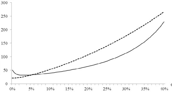
Figure 1: The timing of purchase and the associated gain for various levels of volatility This graph shows the timing of purchase and the associated gain for a buyer attending at the foreclosure sale for various levels of volatility of housing price inflation. The solid curve shows the critical level of the value of the property that triggers the buyer to make an immediate purchase, *
b
V defined in Equation (19), and the dotted
curve shows * 1( b)
F V (scaled up 100 times) defined in Equation (20), which is the gain at the date of purchasing. The benchmark parameter values are given by the irreversible transaction cost K1 unit, the redemption period
1
T year, the parameter for the buyer’s managerial ability 0.05, the expected rate of housing price inflation
1%
per year, and the discount rate r6% per year.
Figure 1 shows the result for the case where the volatility of housing price inflation, , changes in a region between 0% to 40% per year. We see that there exists a turning point at
3%
per year. As the volatility increases, the potential loss incurred by a buyer resulting
15 The transaction cost relative to the purchase price is equal to 1/64.51 = 1.55%, which is plausible as it is smaller than that spent in purchasing a property not subject to the foreclosure sale, i.e., 5% – 6% (Stokey, 2009).
21
from the repurchase option owned by the mortgagor also increases. Consequently, the buyer’s
gain from an immediate purchase and the option value from waiting will both decrease.
When uncertainty is very insignificant (i.e., the volatility is smaller than 3% per year), the
reduction in the former is less than the reduction in the latter such that the buyer will speed up
purchasing. This contrasts with the situation when uncertainty is significant (i.e., the volatility
is greater than 3%) because the loss resulting from the right for the mortgagor to redeem
his/her foreclosed property is sufficiently high such that the buyer will wait longer before
purchasing. Given that the volatility of housing price inflation less than 3% per year is
uncommon in most real estate markets, we thus predict that a buyer is less likely to bid if
housing price inflation fluctuates more severely. Nevertheless, without considering the time
value of money, the gain for the buyer at the date of purchasing will unambiguously increase
22
Table 1
Optimal timing of purchase and the associated gain at the date of purchase Benchmark case: 20%, 1%, K1, T1, 0.05, and r6%
Panel A: Variation in -1% 0% 1% 2% 3% * b V 52.45 57.17 64.51 76.58 98.57 * 1( b) F V 0.647 0.817 1.073 1.485 2.226 Panel B: Variation in K 0.5 0.75 1.0 1.25 1.5 * b V 32.25 48.38 64.51 80.63 96.76 * 1( b) F V 0.536 0.805 1.073 1.341 1.609 Panel C: Variation in T 0.5 0.75 1 1.25 1.5 * b V 48.37 54.73 64.51 80.60 110.9 * 1( b) F V 1.073 1.073 1.073 1.073 1.073 Panel D: Variation in 0.03 0.04 0.05 0.06 0.07 * b V 130.58 85.91 64.51 51.97 43.75 * 1( b) F V 1.043 1.058 1.073 1.088 1.103 Panel E: Variation in r 0.04 0.05 0.06 0.07 0.08 * b V 80.35 70.58 64.51 60.30 57.17 * 1( b) F V 1.577 1.265 1.073 0.941 0.844
Notes: The terms , , K, T, , and r are exogenous variables, which denote the volatility of the expected appreciation rate of
housing prices per year, the expected appreciation rate of housing prices per year, the transaction cost (in unit), the length of statutory
redemption (year), the parameter for the buyer’s managerial ability, and the discount rate per year, respectively. The terms * b
V and F V1( b*)
are endogenous variables, which denote the critical level of the property value that triggers a buyer to purchase the foreclosed property at
0
t , and the associated gain at the purchasing date, respectively.
The results conform to the theoretical results stated in Propositions 1, 2, and 3. Panel A
23
varies from -1% to 3% per year. It shows that a buyer who expects housing prices to
appreciate more rapidly in the future will lose more if making an immediate purchase than if
delaying the purchase. Consequently, the buyer will postpone purchasing, thus gaining more
at the date of purchasing.
Panel B shows the result for the case where the irreversible transaction cost, K , varies
from 0.5 units to 1.5 units. A buyer who incurs larger transaction costs in purchasing a
foreclosed property will delay purchasing, and thus will gain more at the date of purchasing.
However, after considering the time value of money, the gain associated with purchasing will
decrease with the transaction cost.
Panel C shows the result for the case where the statutory redemption period, T , varies
from a half year to one and half years. As expected, a longer statutory redemption period
encourages the buyer to delay purchasing, but leaves unchanged the gain at the date of
purchasing. However, a longer statutory redemption period will reduce the gain from
purchasing after we take the time value of money into account.
Panel D shows the result for the case where a buyer can increase the value of the
purchased property by 3% to 7%, i.e., varies from 0.03 to 0.07. As a buyer is more capable in enhancing the value of the bought property, the buyer will speed up purchasing
because the gain from purchasing will more than offset the increase of the potential loss
24
expected, at the purchasing date the buyer’s gain is increasing with the buyer’s managerial
ability.
Finally, Panel E shows the result for the case where the buyer’s discount rate, r, varies
from 4% to 8% per year. It shows that a far-sighted buyer (low r) will delay and thus gain
more from the purchase.
6. Conclusion
About one third of states in the U.S. offer the right of statutory redemption to a
defaulting mortgagor who can reclaim his/her foreclosed property within a certain period of
time, usually lasting for one month to one year. We derive a closed-form solution of a buyer’s
decision at the foreclosure sale, which predicts that the buyer is less likely to purchase in
states with statutory redemption than in states without it. In states with statutory redemption, a buyer’s likelihood to purchase will decline if the redemption period lasts longer or housing price inflation fluctuates more severely because the buyer will then be hurt more by the
defaulting mortgagor who owns more valuable repurchasing option.
To test our predictions, researchers need to collect empirical data on both the dependent and independent variables. For the former researchers need to use data to proxy a buyer’s likelihood to purchase. We suggest that “the average number of auctions being taken place for settling down a foreclosed property” could be such a proxy. For the independent variables, we
25
suggest that researchers can collect the state-level data on the statutory redemption period
from Baker, Miceli, and Sirmans (2008), and the metropolitan-level data on the housing price
volatility from Miller and Peng (2004). We, however, leave future work to test our
predictions.
Our predictions come from a very simplified model, which can be extended in the
following ways. First, we may consider the default decision made by a mortgagor, and thus
also take the equitable right of redemption into account. Second, we may allow more buyers
to compete at the foreclosure sale rather than consider only one single buyer. The game
played by the buyers and the mortgagor will then become a hierarchical one (Jou, 2004;
Krawczyk and Zaccour, 1999). Third, we may allow an auctioneer to lower his/her
reservation price each time when resetting the date for the foreclosure sale. Finally, we have
not discussed whether it is desirable to eliminate or shorten the period of statutory redemption
(see, e.g., Phillips and Rosenblatt, 1997). We may take the objective function of the regulator
into account in order to investigate this issue. We leave these extensions to future research.
Acknowledgements
We would like to thank the Editor (Carl R. Chen), two anonymous reviewers, and
seminar participants at the 16th New Zealand Finance Colloquium held in Massey University
(Albany Campus) in Feb., 2012 and 4th Annual Conference of Global Chinese Real Estate
26 References
Asabere, P. K., & Huffman, F. E. (1992). Price determinants of foreclosed urban land. Urban
Studies, 29(5), 701-707.
Baker, M. J., Miceli, T. J., & Sirmans, C. F. (2008). An economic theory of mortgage
redemption laws, Real Estate Economics, 36(1), 31-45.
Barone-Adesi, G., & Whalley, R. E. (1987). Efficient analytic approximation of American
option values, Journal of Finance, 42, 301-320.
Black, F., & Scholes, M. (1973). The pricing of options and corporate liabilities. Journal of
Political Economic, 3, 637-659.
Brueggeman, W. B., & Fisher, J. D. (2006). Real Estate Finance and Investments (13th
edition), McGraw-Hill: New York, NY, 10020.
Carr, P. (1995). The valuation of American exchange options with application to real options.
In Lenos Trigeorgis (Ed.), Real Options in Capital Investment, 109-120, Praeger.
Clauretie, T. M. (1987). The impact of interstate foreclosure cost differences and the value of
mortgages on default rates, AREUEA Journal, 15(3), 152-167.
Clauretie, T. M., & Herzog. T. (1990). The effect of state foreclosure laws on loan losses:
Evidence from the mortgage insurance industry, Journal of Money, Credit, and Banking,
27
Cox, J. C., & Ross, S. A. (1976). The valuation of options for alternative stochastic process.
Journal of Financial Economics 3(1), 145-166.
Dixit, A. K., & Pindyck, R. S. (1994). Investment under Uncertainty, Princeton University
Press, New Jersey.
Fischer, E. O. (1993). Analytic approximation for the valuation of American put options on
stocks with known dividend. International Review of Economics and Finance, 2(2),
115-127.
Geske, R. L., & Johnson, E. (1984). The American put option values analytically. Journal of
Finance, 39, 1511-1524.
Goetzmann, W. N., & Ibbotson, R. G. (1990). The performance of real estate as an asset class.
Journal of Applied Corporate Finance, 3(1), 65-76.
Grenadier, S. R. (2002). Option exercise games: An application to the equilibrium investment
strategies of firms. Review of Financial Studies, 15(3), 691-721.
Jaffee, A. (1985). Mortgage foreclosure law and regional disparities in mortgage financing
costs. Working paper no. 85-80, Pennsylvania State University.
Jou, J.-B. (2004). Environment, irreversibility and optimal effluent standards. The Australian
Journal of Agricultural and Resource Economics, 48(1), 127-158.
28
an oligopoly. Journal of Financial and Quantitative Analysis, 43(3), 769-786.
Jou, J.-B., & Lee, T. (2009). How does a development moratorium affect development timing
choices and land values? Journal of Real Estate Finance and Economics, 39, 301-315.
Kau, J. B., Keenan, D. C., & Kim, T. (1993). Transactions Costs, Suboptimal Termination and
Default Probabilities. Journal of the American Real Estate and Urban Economics
Association, 24(3), 279-299.
Kau, J. B., Keenan, D. C., & Smurov, A. A. (2011). Leverage and mortgage foreclosures.
Journal of Real Estate Finance and Economics, 42, 393-415.
Krawczyk, J. B., & Zaccour, G. (1999). Management of pollution from decentralized agents
by local government. International Journal of Environment and Pollution, 12, 343-357.
Lee, J., & Paxson, D. A. (2003). Confined exponential approximations for the valuation of
American options. European Journal of Finance, 9, 449-474.
Meador, M. (1982). The effect of mortgage laws on home mortgage rates. Journal of
Economics and Business, 34, 143-148.
Merton, R. C. (1973). The theory of rational option pricing. Bell Journal of Economics and
Management Science, 4, 141-83.
Miceli, T. J., & Sirmans, C. F. (2005). Time-limited property rights and investment incentives.
29
Miller, N. & Peng, L. (2006). Exploring Metropolitan Housing Price Volatility. Journal of
Real Estate Finance and Economics, 33(1), 5-18.
Phillips, R. A., & Rosenblatt, E. (1997). The legal environment and the choice of default
resolution alternatives: an empirical analysis. Journal of Real Estate Research, 13(2),
145-154.
Phillips, R. A., & VanderHoff, J. H. (2004). The conditional probability of foreclosure: an
empirical analysis of conventional mortgage loan defaults. Real Estate Economics,
32(4), 571-587.
Reinsdorf, M. (1994). New Evidence on the Relation Between inflation and Price Dispersion,
American Economic Review, 84(3), 720-731.
Stokey, N. L. (2009). The Economics of Inaction, Princeton University Press, New Jersey.
Wong, K. P. (2006). The Effects of Abandonment Options on Operating Leverage and Forward Hedging, International Review of Economics and Finance, 15(1), 72-86.
Wong, K. P. (2009). The Effects of Abandonment Options on Operating Leverage and Investment timing, International Review of Economics and Finance, 18(1), 162-171.
30
Table 1 presents the comparative-statics results, in which only one parameter is changed around its benchmark value, while the other parameters are held at their benchmark values.