s
. _-
..
!B
&d
1
ELSEVIER
A consistent
Comput. Methods Appl. Mech. Engrg. 156 (1998) 259-276
Computer methods
in
applied mechanics andengineering
finite element formulation for linear buckling analysis
of spatial beams
K.M. Hsiao*,
R.T. Yang, W.Y. Lin
Department of Mechanical Engineering, National Chiao Tung University, Hsinchu, Taiwan, ROC
Received 17 March 1997; revised 1.5 May 1997
Abstract
A consistent co-rotational finite element formulation and numerical procedure for the linear buckling analysis of three-dimenslonal elastic Euler beam is presented. A mechanism for generating configuration dependent conservative moment is proposed and the corresponding load stiffness matrix is derived. It is assumed that the prebuckling displacements and rotations of the structure and the corresponding deformations of the elements are linearly proportional to the external loading. The prebuckling rotations of the structure are fixed axis rotations or small rotations, and the effect of the prebuckling displacement on transformation matrix for the coordinates transformation can be ignored. All coupling among bending, twisting and stretching deformations for beam element is considered by consistent linearization of the fully geometrically nonlinear beam theory. An inverse power method for the solution of the generalized eigenvalue problem is used to find the buckling load and buckling mode. Numerical examples are presented to demonstrate the accuracy and efficiency of the proposed method. 0 1998 Elsevier Science S.A.
1. Introduction
The linear buckling analysis has been the subject of considerable research, and many valuable results have been reported in the literature [l- 131. The buckling of the beam structures is caused by the coupling among bending, twisting and stretching deformations of the beam members. Thus, the buckling analysis is known as a second-order analysis [l]. In order to capture correctly all coupling among bending, twisting and stretching deformations of the beam elements, the formulation of beam elements might be derived by consistent linearization of the fully geometrically nonlinear beam theory [14]. However, the governing equations of conventional linear buckling analysis are not derived from the consistent linearization of the fully geometrically nonlinear beam theory. Thus, the conventional linear buckling analysis cannot account for the complete deformational coupling. A large number of nonlinear models of thin-walled beams has been proposed (e.g. see the references in [ 151). However, most of them are applied to the non-linear analysis of beams. Their application in the linear buckling analysis has been rather limited (e.g. [ 12,131. To the authors’ knowledge, it seems that their governing equations are not obtained by consistent linearization of the fully geometrically nonlinear beam theory. The objective of this study is to present a consistent co-rotational finite eiement formulation and numerical procedure for the linear buckling analysis of three-dimensional elastic Euler beam using consistent linearization of the fully geometrically nonlinear beam theory. In [ 161, Hsiao presented a co-rotational total Lagrangian formulation of beam element for the nonlinear analysis of three-dimensional beam structures with large rotations but small strains. All coupling among bending, twisting and stretching deformations for beam element is correctly considered by the fully geometrically nonlinear beam theory. Element deformations and
* Corresponding author.
0045-7825/98/$19.00 0 1998 Elsevier Science S.A. All rights reserved
260 K.M. Hsiao et al. I Comput. Methods Appl. Mech. Engrg. 156 (1998) 259-276
element equations are defined in terms of element coordinates which are constructed at the current configuration of the beam element. The element deformations are determined by the rotation of element cross section coordinates, which are rigidly tied to element cross section, relative to the element coordinate system. In conjunction with the co-rotational formulation, the higher-order terms of nodal parameters in element nodal force and stiffness matrix are consistently dropped. It seems that this element can be adapted for the linear buckling analysis of the beam structures. Thus, the beam element presented in [16] is modified and employed here.
The configuration dependent conservative moment is considered and the corresponding load stiffness matrix is derived. It is assumed that the prebuckling displacements and rotations of the structure and the corresponding deformations of the elements are linearly proportional to the external loading. The prebuckling rotations of the structure are fixed axis rotations or small rotations, and the effect of the prebuckling displacement on transformation matrix for the coordinates transformation can be ignored. An inverse power method for the solution of the generalized eigenvalue problem is used to find the buckling load and buckling mode. Numerical examples are presented to demonstrate the accuracy and efficiency of the proposed method.
2.
Finite element formulation
In the following only a brief description of the beam element is given. The more detailed description may be obtained from [16].
2.1.
Basic assumptionsThe following assumptions are made in derivation of the beam element behavior. (1) The beam is prismatic and slender, and the Euler-Bernoulli hypothesis is valid. (2) The cross section of the beam is doubly symmetric.
(3) The unit extension and the twist rate of the centroid axis of the beam element are uniform.
(4) The cross section of the beam element does not deform in its own plane and strains within this cross section can be neglected.
(5) The out-of-plane warping of the cross section is the product of the twist rate of the beam element and the Saint Venant warping function for a prismatic beam of the same cross section.
(6) The deformations of the beam element are small.
2.2. Coordinate systems
In this paper, a co-rotational total Lagrangian formulation is adopted. In order to describe the system, we define four sets of right handed rectangular Cartesian coordinate systems:
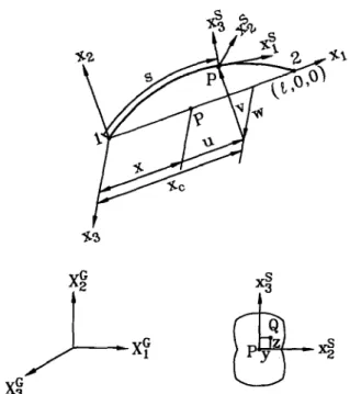
(1) A fixed global set of coordinates, Xc (i = 1,2, 3) (see Fig. 1); the nodal coordinates, displacements, and rotations, and the stiffness matrix of the system are defined in this coordinates.
(2) Element cross section coordinates, xf (i = 1,2,3) (see Fig. 1); a set of element cross section coordinates is associated with each cross section of the beam element. The origin of this coordinate system is rigidly tied to the shear center of the cross section. The ZK~ axes are chosen to coincide with the normal of the unwrapped cross section and the xi and .x: axes are chosen to be the principal directions of the cross section.
(3) Element coordinates, xi (i = 1,2,3) (see Fig. 1); a set of element coordinates is associated with each element, which is constructed at the current configuration of the beam element. The origin of this coordinate system is located at node 1, and the x, axis is chosen to pass through two end nodes of the element; the x2 and x3 axes are chosen to be the principal directions of the cross section at the undeformed state. Note that this coordinate system is a local coordinate system not a moving coordinate
system. The deformations, internal nodal forces and stiffness matrix of the elements are defined in terms of these coordinates. In this paper the element deformations are determined by the rotation of element cross section coordinate systems relative to this coordinate system.
KM. Hsiao et al. I Comput. Methods Appl. Mech. Engrg. 156 (1998) 259-276 261
Fig. I. Coordinate systems.
(4) Load base coordinates, Xp (i = 1,2,3);
a set of load base coordinates is associated with each
configuration dependent moment. The origin of this coordinate system is chosen to be the node where the
configuration dependent moment is applied. The mechanism for generating configuration dependent
moment is described in this coordinates, and the corresponding external load and load stiffness matrix are
defined in terms of this coordinates.
In this paper, the symbol { } denotes column matrix. The relations among the global coordinates, element
cross section coordinates, element coordinates and load base coordinates may be expressed by
XG=AG#,
XG=A,$,
XG = AGpXP(1)
where Xc = {XF, XF, X,“}, xS = {xf, xi, xs}, x = {xi, x2, x,}, and Xp = {Xp, X:, X:}; A,,, A,,
and AGP are
matrices of direction cosines of the element cross section coordinate system, element coordinate system, and
load base coordinate system, respectively.
2.3.
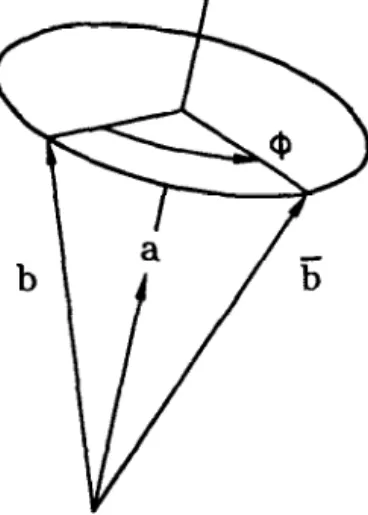
Rotation vector and rotation parametersFor convenience of the later discussion, the term ‘rotation vector’ is used to represent a finite rotation. Fig. 2
shows that a vector b which as a result of the application of a rotation vector + is transported to the new
position b. The relation between b and b may be expressed as
[171
b=cos&+(l-cos~$)(u~b)+sinf#@Xb)
(2)
where 4 is the angle of counterclockwise rotation, and a is the unit vector along the axis of rotation.
Let ej and es
(i =1,2,3) denote the unit vectors associated with the xi and $ axes, respectively. Here, the
traid es in the deformed state is assumed to be achieved by the successive application of the following two
rotation vectors to the traid ei:
0, = e,n
(3)
and
262 K.M. Hsiao et al. I Comput. Methods Appl. Mech. Engrg. 156 (1998) 259-276
Fig. 2. Rotation vector
where
n = (0, e&e;
+ 0:)“2, e&e;
+ rQ1’*]
= (0, n2, nJ
(5)
t =
{cos
en,
e,,
4,)
(6)
cos 0, = (1 - f?; -
oy
(7)
dW
O, = -
ds 7in which n is the unit vector perpendicular to the vectors e, and es and t is the tangent unit vector of the
deformed centroid axis of the beam element. Note that es coincides with t. 0, is the inverse of cos 6”. u(s) and
W(S) are the lateral deflections of the centroid axis of the beam element in the x2 and xg directions, respectively,
and s is the arc length of the deformed centroid axis.
Using Eqs. (2)-(8), the relation between the vectors e, and es (i = 1,2,3) in the element coordinate system
may be obtained as
ef = [t,
R,, R,]e, = Re,
(9)
R, =cosd,rl
+sinO,r,,
R, = -sin 8,r, + cos 0, r2
r, = {-f3,, cos 0, + (1 - cos O,>ni, (1 - cos 6,)n,n,>
r2 = {0,, (1 - cos O,>n,n,, cos 0, + (1 - Cos O,,)rz:>
(10)
where R is the so-called rotation matrix. The rotation matrix is determined by bi (i = 1,2,3). Thus, 0, are called
rotation parameters in this study.
Let 8 = {Or, o,, 0,) be the column matrix of rotation parameters, 68 be the variation of 6. The tmid ef
(i = 1,2,3) corresponding to 8 may be rotated by a rotation vector &#J = (64,)
S&, S+,> to reach their new positionscorresponding to 8 + 68
[161. When 0, and 0, are much smaller than unity, the relationship between 68
and SC+ may be approximated by [161
-412
0
1
6&=T-%$.
(11)
K.M. Hsiao et al. 1 Comput. Methods Appl. Mech. Engrg. 156 (1998) 259-276 263
2.4. Nodal parameters and forces
The element employed here has two nodes with six degrees of freedom per node. Two sets of element nodal parameters termed ‘explicit nodal parameters’ and ‘implicit nodal parameters’ are employed. The explicit nodal parameters of the element are used for the assembly of the system equations from the element equations. They are chosen to be ujj, the x, (i = 1, 2,3) components of the translation vectors uI at node j(j = 1,2) and +ij, the x, (i = 1, 2,3) components of the rotation vectors +j at node j(j = 1,2). Here, the values of 4j are reset to zero at current configuration. Thus, SC$~~, the variation of 4,j, represent infinitesimal rotations about the xi axes [16], and the generalized nodal forces corresponding to S+ij are m,,, the conventional moments about the x< axes. The generalized nodal forces corresponding to Suij, the variation of ulj, are J;,, the forces in the x, directions.
The implicit nodal parameters of the element are used to determine the deformation of the beam element. They are chosen to be u;,, the x1 (i = 1,2, 3) components of the translation vectors u, at node j (j = 1,2) and qj, the nodal values of the rotation parameters fl (i = 1,2,3) at node j (j = 1,2). The generalized nodal forces corresponding to Suij and Sflj are J;, and ml, the forces in the x, directions and the generalized moments, respectively. Note that rnt. are not conventional moments, because SO, are not infinitesimal rotations about the x, axes at deformed state.
In view of Eq. (1 l), the relations between the variation of the implicit and explicit nodal parameters maybe expressed as
(12)
where Su, = {SU,~, SuZj, SuJj}, Sg = {SO,,, SOZj, S13~~3j) and S4j = {SC&,, C&j, S&j, (j = 1,2); Z and 0 are the identity and zero matrices of order 3 X 3, respectively; T,:’ (j = 1,2) are nodal values of T - ’ given in Eq. ( 11).
Let f= If,,
m,,
f,,
m2>, f,
= if,,
mf,
.f,,m:l,
M,,
m$, mlj}
(j
=
1, 2), denote the internal nodal force vectors correspondingwhere
J;.
= {fij,
Ljr
f,>,
mj = {m,p
to the variation of the explicitm2p
m3,,19
and my =
and implicit nodal parameters, Sq and Sqe, respectively. Using the contragradient law [18] and Eq. (12) the relation betweenf
andf,,
may be given byf=Ti&
(13)The global nodal parameters for the system of equations corresponding to the element local nodes j ( j = 1, 2) should be consistent with the element explicit nodal parameters. Thus, they are chosen to be U,,, the Xi (i = 1, 2, 3) components of the translation vectors ZJ, at node j (j = 1,2) and qj, the X, (i = 1, 2,3) components of the rotation vectors q. at nodes j (j = 1,2). Here, the values of q. are reset to zero at current configuration. Thus, Sqj, the variation of qj, represent infinitesimal rotations about the Xi axes [ 161, and the generalized nodal forces corresponding to SqY are the conventional moments about the X, axes. The generalized nodal forces corresponding to SU,,, the variation of U,, are the forces in the X! directions.
2.5. Kinematics of beam element
The deformations of the beam element are described in the current element coordinate system. From the kinematic assumptions made in this paper, the deformations of the beam element may be determined by the displacements of the centroid axis of the beam element, orientation of the cross section (element cross section coordinates), and the out-of-plane warping of the cross section. Let Q (Fig. 1) be an arbitrary point in the beam element, and P be the point corresponding to Q on the centroid axis. The position vector of point Q in the undeformed and deformed configurations may be expressed as
rO =.xe, fye, +ze, (14)
and
264 K.M. Hsiao et al. I Comput. Methods Appl. Mech. Engrg. 156 (1998) 259-276
where x,(s), u(s) and w(s) are the x1, x2 and
x j
coordinates of point
P, respectively,s is the arc length of the
deformed centroid axis measured from node 1 to point
P.The relationship among x,(s), u(s), W(S) and s may be
given as
I
sx,(s)= u,, +
cos 8, ds0
(16)
where u,, is the displacement of node 1 in the x, direction, and cos 13, is defined in Eq. (7). Note that due to the
definition of the element coordinate system, the value of u
1 1is equal to zero. However, the variation of
u, ,is
not zero. Making use of Eq. (16), one obtains
2&
cos
en
d{
(17)
e =
x,(S) -
x,(O) =
L - U] 1 + u*2(18)
and
+1+$
(19)
in which S and 8 are the current arc length and chord length of the centroid axis of the beam element,
respectively, and L is the chord length of the undeformed beam axis.
Here, the lateral deflections of the centroid axis u(s) and W(S) are assumed to be the Hermitian polynomials of
s, and the rotation about the centroid axis 19~
(s) (Eq. (3)) is assumed to be linear polynomials of s. u(s), w(s) and
13,(s) may be expressed by
where uZj and u3, (j = 1,2) are nodal values of u and w at nodes j, respectively, and el, (i = 1,2,3, j = 1,2) are
nodal values of @ at
nodes j.Note that, due to the definition of the element coordinates, the values of u2j and LQ~
(j = 1,2) are zero. However, their variations are not zero. N, (i = l-6) are shape functions and are given by
N, =
$
Cl-
5>2(2
+
51,
N~=~~1-52)(1-5),
Nj =
$
(1 +
02(2 -
0,
N,=;(-1+&2)(1+&,
&=&l-C),
Ne=;(l+&.
The axial displacements of the centroid axis may be determined from the lateral deflections
extension of the centroid axis using Eq. (16).
(21)
and the unit
If X, y and z in Eq. (14) are regarded as the Lagrangian coordinates, the Green strain E,
!, q2and E,~ are
given by [19]
811 = + (r:r,, -
1)
Using the chain rule
r,X = r,(l + co)
for differentiation,
txin Eq. (22) may be expressed as
K.M. Hsiao et al. / Comput. Methods Appl. Mech. Engrg. 156 (1998) 259-276 265
(24)
where &(, is the unit extension of the centroid axis. Making use of the assumption of uniform unit extension, one may rewrite Eq. (24) as
S &,)=x- 1 .
Substituting Eqs. (5)-( IO), (15), (23), (25) into Eq. (22), c,, , q2 and E,~ can be calculated. 6, , , E,* and F,~ are given in [ 161 and are not repeated here.
2.6. Element nodal force vector
The element nodal force vectorf, (Eq. (13)) corresponding to the implicit nodal parameters are obtained from the virtual work principle in the current element coordinates. It should be mentioned again that the element
coordinate system is a local coordinate system not a moving coordinate system. Thus, a standard procedure is
used here for the derivation of f,. For convenience, the implicit nodal parameters are divided into four generalized nodal displacement vectors ui (i = a, 6, c, d), where
II, = {U,,? u12] (26)
and uh, uC and ud are defined in Eq. (20).
The generalized force vectors corresponding to 6u,, the variation of ui (i = a, b, c, d) are
f, = {A7
mf,,
.fk
4J
JI
=f.h19m5,~.tL~mZNJ
f, =
hP,
3mPJ
.
The virtual work principle requires that %A, + WJ, + W.& +
wlfd
=
I V (all SC,, + 2u,,, 6s,, + 2a,, 8QdV
(27)
where V is the volume of the undeformed beam, gi, = EC,, , CT,~ = 2Gs, *, and u,~ = AGE,,, where E is the Young’s modulus and G is shear modulus.
If the element size is chosen small enough, the values of the nodal parameters (displacements and rotation parameters) of the element defined in the current element coordinate system may always be much smaller than unity. Thus, the higher-order terms of nodal parameters in the element internal nodal forces may be neglected. However, in order to include the nonlinear coupling among the bending, twisting, and stretching deformations, the terms up to the second order of nodal parameters are retained in element internal nodal forces by consistent linearization of Eq. (28). The nodal force vectors J; (i = a, b, c, d) are given in [ 161 and not repeated here. 2.7. Element tangent stiffness matrices
The element tangent stiffness matrix corresponding to the explicit nodal parameters (referred to as explicit tangent stiffness matrix) may be obtained by differentiating the element nodal force vector f in Eq. ( 13) with respect to explicit nodal parameters. Using Eqs. (12) and (13), we obtain
where k, =
dfo/ aq,
is the tangent stiffness matrix corresponding to implicit nodal parameters (referred to as implicit tangent stiffness matrix), and H is a unsymmetrical matrix and is given by266 K.M. Hsiao et al. / Comput. Methods Appl. Mech. Engrg. 156 (1998) 259-276 1 in which 0 is a (30) 0 0 0 0 H, 0 1
zero matrix of order 3 X 3 and
0 0 m31 --m,j 1 O TrnYi 0
1
(31) 1 0 -- 2 m,iUsing the direct stiffness method, the implicit tangent stiffness matrix k, may be assembled by the submatrices
k,=$
I
(32) where J; (i = a, b, c, d) are defined in Eq. (27) and ui (i = a, b, c, d) are defined in Eqs. (20) and (26). k,, are given in [ 161, and are not repeated here. It is noted that the element tangent stiffness matrix k in Eq. (29) is unsymmetrical. This observation is consistent with that of Simo and Vu-Quoc [20] and Crisfield [21] who adopted different formulation. However, numerical experiments of the present authors have shown that for conservative problems the tangent stiffness matrix of the structure become symmetrical at equilibrium configuration. This observation is again consistent with the theory of Simo and Vu-Quot.
Note that because only the terms up to the second order of nodal parameters are retained in f,, only the terms up to the first order of nodal parameters are retained in the element stiffness matrix given in Eq. (29). Thus the element stiffness matrix in Eq. (29) may be rewritten symbolically as
k=k,+k, (33)
where k, comprises all zeroth order terms of nodal parameters in k and k, comprises all first-order terms of nodal parameters in k. k, is the linear stiffness matrix of elementary beam element, and k, is the geometrical stiffness matrix.
Note that the element coordinate system is only a local coordinate system not a moving or rotating coordinate system here. Thus, the element tangent stiffness matrix referred to the global coordinate system is obtained by using the standard coordinate transformation and may be expressed by
kc = T,,kT;, (34)
TGE=[; j- AiE A!,l (35)
where 0 is a zero matrix of order 3 X 3 and A,, is defined in Eq. (1). 2.8. Load stifness matrix
Different ways for generating configuration dependent moment were proposed in the literature [5,6]. Here, for simplicity, only the conservative moments generated by conservative force or forces (with fixed directions) are considered, and two possible ways for generating conservative moment are employed. In this study, a set of load base coordinates Xp (i = 1,2,3) associated with each configuration dependent moment are constructed at the current configuration. The mechanism for generating configuration dependent moment is described in this coordinates, and the corresponding external load and load stiffness matrix [22] are defined in terms of this coordinates. Unless stated otherwise, all vectors and matrices in this section are referred to this coordinates. Note that this coordinate system is just a local coordinate system constructed at the current configuration, not a
KM. Hsiuo et al. I Comput. Methods Appl. Mech. Engrg. 156 (1998) 259-276 261
moving coordinate system. Thus, it is regarded as a fixed coordinated system in the derivation of the load stiffness matrix.
The first way for generating configuration dependent moment may be described as follows.
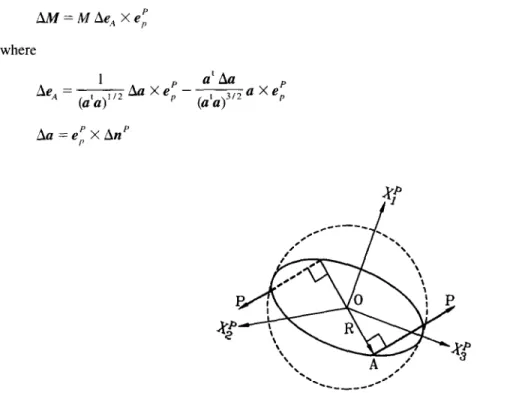
Consider a sphere of radius R which centroid is rigidly connected with the structure at node 0 as shown in Fig. 3. Two strings wound around a great circle of the sphere are acted upon by forces of magnitude I? Thus, the strings are always tangent to the sphere. The great circle and the forces are on the same plane at the undeformed configuration of the structure. However, the great circle and the forces are generally not on the same plane when the structure is deformed. The origin of the load base coordinate system is chosen to be located at the node 0. The Xr axis is chosen to coincide with the normal of the plane of the great circle, and the Xc and Xp axes lie in the plane of the great circle.
Let A denote the contact point of the force P and the great circle. Because P is tangent to the sphere, P is perpendicular to the line OA. Let eA denote unit vector in the direction of line OA. eA may be expressed by
e,, = ~/@‘a)“’ (36)
a=e,PXn’ = (0, (3, - .e*> (37)
where e,’ = {6,, kY2, CT} is th e unit vector in the direction of P, and 12’ is the unit normal of the plane of the great circle. Note that np coincides with ef = (1, 0, 0}, the unit vector associated with the XT axis.
The external moment vector at node 0 generated by the above mentioned mechanism may be expressed by
M=Me, Xe,P (38)
where M = 2RP is the magnitude of the moment.
The moment in Eq. (38) is rotation dependent. When an incremental rotation vector Avp = {Acp,, Ap2, A& passing through node 0 is applied to the sphere, the unit normal of the plane of the great circle, rzp has an incremental change AnP. If the magnitude of A4pp is small enough, AnP may be expressed as
An’ = Aqp X np = (0, APT, -Ap2}. (39)
Note that Aqp is not applied to the load base coordinates here. The incremental moment corresponding to A+D’
may be expressed by
hM=MAe,., Xeg (40)
where
Ae, = a Xe;
Aa=eiXAnP
Fig. 3. Mechanism for generating configuration dependent moment.
(41) (42)
268 K.M. Hsiao et al. I Comput. Methods Appl. Mech. Engrg. 156 (1998) 259-276
Using the tangent stiffness approach, the relation between the incremental moment AM and the corresponding
load stiffness matrix
k,may be expressed as
AM=k,&op.
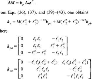
From Eqs. (36), (37), and (39)-(43), one obtains
k, = M( e; + e:)-“*kpa + M( e; + e;)-3’2kph
(43)
(44)
where
04 f3
- e, e2
kpa= 0 [ eze3 e; + e;(45)
0
-e;-e;
-
e2 e3
1
I
0 -e, e3( e; + e;) e, e2e,<
e; + e:)
k,, = 0 e:e2e3 -e;e;
(46)
0
efeg
-efe2e3
1
Three special cases shown in Fig. 4 are considered here. Following [5], they are referred to as quasitangential
(QT) moments of the first and second type, and semitangential (ST) moment. The load stiffness matrices
corresponding to QT and ST moment at the configurations shown in Fig. 4 may be obtained from Eqs.
(44)-(46) and given by
0 0 0 k,QT’=MO 0 0 [ 0-1
0
1
0 0 0 k,QT’=M [ 00 0 0
01
1
k;‘+
[ 0 0 0 0 01
0-1
0
1
(47)
(48)
(49)
The second way for generating configuration dependent moment may be described as follows.
Consider a rigid arm of length
Rwhich end is rigidly connected with the structure at node 0 as shown in Fig.
5. The other end of the rigid arm is acted upon by a conservative force (with a fixed direction) of magnitude P.
The origin of the load base coordinates Xt (i = 1,2,3) is chosen to be located at the node 0. The XT axis is
chosen to coincide with the axis of the rtgtd arm, and the XI and X: axes are perpendicular to the rigid arm.
XT
P
L
R
I
Rigid arm
0
x:
Xl
Fig. 4. Quasitangential (QT) moment and semitangential (ST) moment.
KM. Hsiao et al. I Comput. Methods Appl. Mech. Engrg. 156 (1998) 259-276 269
The external moment vector at node 0 generated by the above mentioned mechanism may be expressed by
M=RPtPXei (50)
where eg = {8,, eze,, &JJ} is the unit vector in the direction of P and tP is the unit vector in the axial direction of the rigid arm. Note that tP coincides with ep = { 1, 0, 0}, the unit vector associated with the XT axis.
The moment in Eq. (50) is rotation dependent. When an incremental rotation vector Aqp = {Acp,, Apz2, APT} passing through node 0 is applied to the rigid arm, the unit vector tP has an incremental change At’. If the magnitude of App is small enough, At’ may be expressed as
At’ =
Aqpp x tP = (0, Ap,, -a~~}. (51)Note thut App is not applied to the load base coordinates here. The incremental moment corresponding to A+cJ’ may be expressed by
AM = M At’ X e,’
= RPIG Av~ + 4 A4ov -4 A4pzv -4 44.
From Eqs. (43) and (52), the corresponding load stiffness matrix may be expressed as
0
k,=RP [ 0 -8,4 4
0 0 01
. -fi (52) (53)The load stiffness matrix referred to the global coordinate system is obtained by using the standard coordinate transformation and may be expressed by
k,” = A GPkpA ;, (54)
where A,, is the transformation matrix given in Eq. ( 1).
3.
Consistent linear buckling analysis
3.1.
AssumptionsFour assumptions are made in the present buckling analysis and given as follows: (1) The external loading is proportional to one loading parameter.
(2) The prebuckling displacements and rotations of the structure and the corresponding deformations and rigid body rotations of the beam element are linearly proportional to the external loading.
(3) The prebuckling rotations of the structure are rotations about axes with the same fixed direction or small rotations.
(4) The effect of the prebuckling displacements on the transformation matrix for coordinate transformation may be ignored.
3.2. Criterion of the buckling state
Here, the zero value of the tangent stiffness matrix determinant is used as the criterion of the buckling state. Let K,(A) denote the tangent stiffness matrix of the structure corresponding to the loading parameter h. The criterion of the buckling state may be expressed as
D(A) = det(K,( A)( = 0 .
The minimum root of Eq. (55) is the buckling load.
270 K.M. Hsiao et al. I Comput. Methods Appl. Mech. Engrg. 156 (1998) 259-276
3.3. Determination of the tangent st@ness matrix of the structure
The tangent stiffness matrix of the structure corresponding to A is assembled by the element stiffness matrices and load stiffness matrices corresponding to A using direct stiffness method. The element tangent stiffness matrix corresponding to A may be determined as follows.
A linear analysis for A = 1 is carried out first. Let uf = {uyj, ut,, &,,> and 44 = {+t,, 4ijy +ijI (j = 1,2) (referred to the initial element coordinates) denote displacement and rotation vectors of an element at node j, which are extracted from the linear solution for A = 1, and then transformed from the global coordinates to the initial element coordinates. The rotation vector corresponding to rotation about axis with fixed direction or small rotation may be regarded as true vector. Thus, making use of assumptions (2) and (3), the rigid body rotation vector of the element +” and the vectors of the deformational rotation parameters 4 at nodes j (j = 1,2) corresponding to uf and 4f (j = 1,2) may be determined by
q =
4” - cp”
(57)where L is the initial length of the beam element. The unit extension of the centroid axis of the beam element may be determined by
1
&” =,(u’;, - uk,). (58)
Making use of assumption (2), and Eqs. (56)-(58), the element tangent stiffness matrix given in Eq. (33) corresponding to loading parameter A referred to the current element coordinates can be calculated and written in the form
k = k, + Nzyf (59)
where kyf IS the geometric stiffness matrix corresponding to A = 1.
The current element coordinates corresponding to loading parameter A can be obtained by the application of the rotation vector A4R to the initial element coordinates. The current load base coordinates corresponding to loading parameter A can be obtained by the application of the rotation vector A4: to the initial load base coordinates, where 4: is the rotation vector at the origin of the load base coordinates, which is extracted from the linear solution for A = 1. However, making use of assumption (4), the initial transformation matrices A,, and A,, constructed at the undeformed structure are used in Eqs. (34) and (54), respectively, for different values of loading parameter A. Thus, the tangent stiffness matrix of the structure is also a linear function of the loading parameter A, and may be written in the form
KT
=
K, +AK:’
(60)
where K, is the linear stiffness matrix of the structure, and Kf”’ is the geometric stiffness matrix of the structure corresponding to A = 1.
3.4. Calculation of the buckling load
From Eq. (60), we know that Eq. (55) is equivalent to the generalized eigenvalue problem
K,Q = -,U(:"'Q
where Q is the eigenvector. The minimum eigenvalue of Eq. (61) is the buckling load and the corresponding eigenvalue is the buckling mode. Here, the inverse power method [23] is use to find the buckling load and buckling mode.
K.M. Hsiao et al. I Comput. Methods Appl. Mech. Engrg. 156 (1998) 259-276 271
4. Numerical studies
EXAMPLE 4.1: Cantilever beam subjected to end force. The example considered here is a cantilever beam
subjected to a lateral end force P as shown in Fig. 6. The Xp (i = 1,2, 3) axes of the global coordinate system shown in Fig. 6 coincide with xf axes, the axes of the element cross section coordinate system in the undeformed beam. The geometry and material properties are: length L = 1 m, cross sectional area A = 3 X lop5 m, moment of inertia about .xi axis Z, = 1.25 X lop9 m4, moment of inertia about $ axis I, = lo-’ m4, torsional constant J = lo-” m4, Young’s modulus E = 1.0 X 10’ N/m*, and shear modulus G = 5 X lO’N/m*. The classical buckling load for this example is P,, = (4.013/Lz)dv = 0.10033 N [3].
The buckling loads of the present study together with the results of [6] and [ 121 are given in Table 1. Very good agreement among all these solutions is observed.
EXAMPLE 4.2: Cantilever beam subjected to end moment. The example considered here is a cantilever beam
subjected to end moment M. The quasitangential and semitangential moments are considered. The corresponding load base coordinates are shown in Fig. 7. The geometry and material properties of the beam are identical with those of Example 1. The classical buckling moment is quoted in [3] as
The buckling loads of the present study together with the finite element results of [6] and [ 121, and analytical solution of [3] are given in Table 2. The results of the present study, [6], and [12] are obtained using ten elements. Very good agreement among all these solutions is observed.
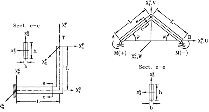
EXAMPLE 3: Cantilever angle subjected to a horizontal end force. The example of the end cross section as
shown in Fig. 8. Here P( +) and P(-) denote forces directed along positive and negative Xp axis, respectively. The geometry and material properties are: L = 240 mm, b = 0.6 mm, h = 30 mm, Young’s modulus E = 71240 N/mm*, and shear modulus G = 27191 N/mm’.
The buckling loads of the present study obtained by using 20 elements for P(+) and P(-) are 1.0880 N and 0.6804 N, respectively. The results of the present study are identical with those results given by Argyris et al. [7] using 20 elements. 8 P
jzq
L ----_-.-_-_ x:Fig. 6. Cantilever beam subjected to lateral load.
Fig. 7. Cantilever beam subjected to end moment.
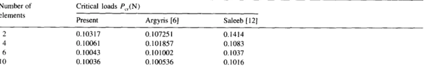
Table 1
Critical load of cantilever beam subiected to end force
Number of elements 2 4 6 10 Critical loads P_(N)
Present Argyris [6] Saleeb (121
0.10317 0.10725 1 0.1414
0.10061 0.101857 0.1083
0.10043 0.101002 0.1037
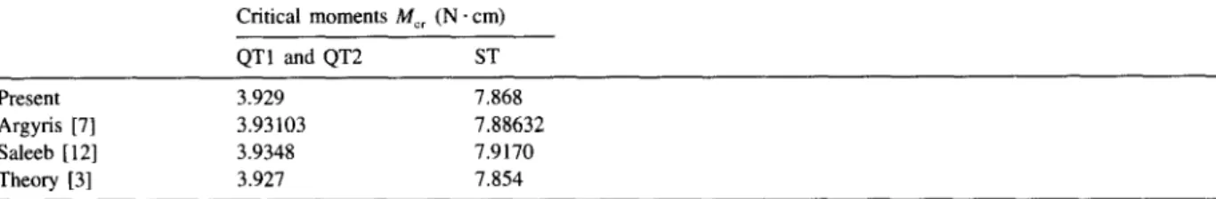
272 K.M. Hsiao et al. I Comput. Methods Appl. Mech. Engrg. 156 (1998) 259-276 Table 2
Critical load of cantilever beam subiected to end moment
Critical moments M,, (N . cm) Present Argyris [7] Saleeb [ 121 Theory [3] QTl and QT2 ST 3.929 7.868 3.93103 7.88632 3.9348 7.9170 3.927 7.854
L-=7l
----_-_____
e-JXS
v
i
Sect.
e-e
i L
XX
41
i P(+) _1__l XZh
4t.-b
Fig. 8. Cantilever angle subjected to a horizontal end force.
Fig. 9. Cantilever angle subjected to end moment.
EXAMPLE 4: Cantilever angle subjected to end moment.
The example considered here is a cantilever angle
subjected to end moment
M.The quasitangential and semitangential moments are considered. The corresponding
load base coordinates are shown in Fig. 9. The geometry and material properties of the beam are identical with
those of Example 1.
The buckling moments of the present study together with the results of [6] and
[121 are given in Table 3. Very
good agreement among all these solutions is observed.
Table 3
Critical moments for cantilever angle with end bending moment
Type of moment
Number of elements
Critical moments M,,(N . cm)
Present Argyris 161 Saleeb [12]
QTl 8 0.4934 0.4935 0.4936 12 0.4935 0.4935 0.4935 20 0.4935 0.4935 0.4935
QT2
8 3.445 3.453 3.467 12 3.439 3.442 3.448 20 3.435 3.437 3.439 ST 8 0.98655 0.98699 0.9878 12 0.98679 0.98698 0.9873 20 0.98691 0.98698 0.987 1KM. Hsiao et al. I Comput. Methods Appl. Mech. Engrg. 156 (1998) 259-276 213 Sect. e-e
Sect.
e-ex”z
x:
4
h --II-- b Fig. 10. Cantilever angle subjected to end torsion.Fig. 11, Simply supported angle frame subjected to uniform moment.
EXAMPLE 5: Cantilever angle subjected to end torsion. The example considered here is a cantilever angle
subjected to end torsion T. The quasitangential and semitangential moments are considered. The corresponding load base coordinates are shown in Fig. 10. Two cases of cross section are considered: (1) b = 0.6 mm, h = 10 mm, (2) b = 10 mm, h = 0.6 mm. The rest geometry and material properties of the angle are: L = 240 mm, Young’s modulus E = 71240 N/mm’, and shear modulus G = 27191 N/mm’.
The present results obtained by using 80 elements are shown in Table 4 together with the results of [lo]. As can be seen, the discrepancy between these two results are remarked for case (1) is observed. Note that the prebuckling displacements for this example is quite large. Thus a nonlinear buckling analysis [6,24,25] may be required for reliable solutions.
EXAMPLE 6: Simply supported angle frame subjected to uniform moment. The example considered here is a
simply supported angle frame subjected to uniform moment M as shown in Fig. 11. Here, M( +) and M(-) denote moments about positive and negative Xr axis, respectively. The ends of the beam are free to rotate about XF axis, but rotation about X$ and Xf axes are prevented. The translation of end point A is restrained, and end points B is free to move in the direction of Xp axis. Because of the rotational boundary conditions used here, the ways of generating end moments are rendered irrelevant here. The material properties are identical with those of Example 3. The theoretical results is M,, E&GJ= 622.21 N* mm [3], which is independent of the angle (p shown in Fig. 11.
Table 4
Critical moment for cantilever with end torsion
Type of moment QT1 QT2 ST Critical moment T,, (N . mm) bXh=0.6mmXlOmm
Present Yang [IO]
262.2 833
271.1 729
274.6 1444
bXh=lOmmX0.6mm
Present Yang [IO]
56.6 60.6
103.1 106.1
214 K.M. Hsiao et al. /
The buckling moment of the present N * mm, respectively, for M( + / -) and using 20 elements.
Comput. Methods Appl. Mech. Engrg. 156 (1998) 259-276
study and results given by [6] and [12] are 624.76, 624.17, and 627.37 M(- / +) and different values of angle q. All these results are obtained
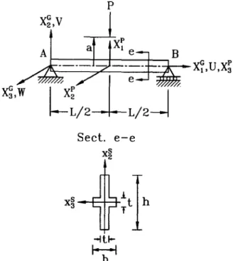
EXAMPLE 7: Simply supported beam subjected to a central concentrated load. The example considered here is
a simply supported beam subjected to a concentrated load P at the middle as shown in Fig. 12. Here, three cases are considered for the application point of P: (1
j
upper face, (2) centroid and (3) lower face. The ends of the beam are free to rotate about Xz and Xy axes, but rotation about Xy axis is restrained. The translation is restrained at end point A, and is free only in the direction of Xp axis at points B. The geometry and materialXF,
Sect. e-e
Fig. 12. Simply supported beam subjected to a central concentrated load.
Table 5
Critical loads for simply supported beam with central concentrated load
Load applied at Upper face L (m) P,,(N) p,,, IP,, a I 2460.03 0.998 2 740.37 1.396 3 529.85 1.083 4 354.51 1.025 5 248.57 1.007 Centroid 1 8382.96 1.000 2 2095.74 1.000 3 931.44 1 DO0 4 523.94 1 BOO 5 335.32 1.000 Lower face 1 19225.96 0.888 2 3451.12 1.013 3 1333.03 1.029 4 693.36 1.028 5 422.06 1.025
K.M. Hsiao et ul. I Comput. Methods Appl. Mech. Engrg. 156 (1998) 259-276 275
properties are: L = 1,
2,
3,
4,
5
m,b
= 0.06
m, h = 0.1 5m, t =0.002
m, Young’s modulusE = 2.04
X 10’ ’ N/m*, and shear modulus G = 7.9 X 10” N/m*. The classical buckling moment is quoted in [3] asP,,
=
0.5 h for upper face for centroid for upper face
The present results obtained by using 40 elements are shown in Table 5 together with the analytical solution of [3]. As can be seen, when the load is applied at the centroid, the results of the present study are identical with those results given in [3]. When the load is applied at the upper face, the maximum discrepancy (39.6%) between these two results occurs at L = 2m.
5. Conclusions
This paper has proposed a consistent linear buckling analysis of three-dimensional elastic Euler beams by using consistent second-order linearization of the fully geometrically nonlinear beam theory. The beam element proposed in 1161 for nonlinear analysis is modified and employed here. All coupling among bending. twisting and stretching deformations for beam element is exactly considered by consistent linearization of the fully geometrically nonlinear beam theory. Based on the assumptions that the prebuckling displacements and rotations are linearly proportional to the external loading, the prebuckling rotations of the structure are fixed axis rotations or small rotations, and the effect of the prebuckling displacement on transformation matrix for the coordination can be ignored, a generalized eigenvalue problem is obtained for linear buckling analysis. An inverse power method for the solution of the generalized eigenvalue problem is used to find the buckling load and buckling mode. Numerical examples are presented to demonstrate the accuracy and efficiency of the proposed method. The agreement between the results of the present study and those given in the literature is very good for most examples. However, for some cases with large prebuckling displacements, the discrepancy between the results of the present study and classical solutions given in the literature is not small. Thus when the prebuckling displacements are not negligible, a nonlinear buckling analysis may be required for reliable solutions.
References
[l] W.F. Chen and E.M. Lui, Structural Stability, Theory and Implementation (Elsevier Science Publishing Co., Inc. NY, 1988). [2] V.Z. Vlasov, Thin Walled Elastic Beams, 2nd edition (English translation published for US. Science Foundation by Israel Program for
Scientific Translations, 1961).
[3] S.P. Timoshenko and J.M. Gere, Theory of Elastic Stability, 2nd edition (McGraw-Hill, NY, 1963).
[4] R.S. Barsoum and R.H. Gallagher, Finite element analysis of torsional and torsional-flexural stability problems, Moments, Int. J. Numer. Methods Engrg. 2 (1970) 335-352.
[5] H. Ziegler, Principles of Structural Stability (Birkhauser, Verlag, Base], 1977).
[6] J.H. Argyris, P.C. Dunne and D.W. Scharpf, On large displacement-small strain analysis of structures with rotation degree of freedom. Comput. Methods Appl. Mech. Engrg. 14 (1978) 401-451; 15 (1978) 99-135.
[7] J.H. Argyris, 0. Hilpert, GA. Malejannakis and D.W. Scharpf, On the geometrical stiffness of a beam in space-A consistent V.W. Approach, Comput. Methods Appl. Mech. Engrg. 20 (1979) 105-131.
[8] J.H. Argyris, H. Balmer, J.St. Doltsinis, P.C. Dunne, M. Haase, M. Kleiber, G.A. Malejannakis, HP Mlejenek, M. Muller and D.W. Scharpf, Finite Element Method-The natural approach, Comput. Methods Appl. Mech. Engrg. 17/18 (1979) l-106.
[9] M.M. Attard, Lateral buckling analysis of beams by FEM, Comput. Struct. 23 (1986) 217-231.
[tOI Y.B. Yang and S.R. Kuo, Buckling of frames under various torsional loading, J. Engrg. Mech., ASCE I17 (1991) 1681-1697. [ 111 Z.P. Bazant and L. Cedolin, Stability of Structures (Oxford University Press, 1991).
[ 121 A.F. Saleeb, T.Y.P. Chang and A.S. Gendy, Effective modeling of spatial buckling of beam assemblages, accounting for warping constraints and rotation-dependency of moments, Int. J. Numer. Methods Engrg. 33 (1992) 469-502.
[13J M.Y. Kim, S.P. Chang and S.B. Kim, Spatial stability analysis of thin walled space frames, Int. J. Numer. Methods Engrg. 39 (1996) 499-525.
[ 141 J.C. Simo and L.Vu-Quoc, The role of non-linear theories in transient dynamic analysis of flexible structures, J. Sound Vib. 1 19 (1987) 487-508.
[ 151 A.S. Gendy and A.F. Saleeb, Generalized mixed finite element model for pre- and post-quasistatic buckling response of thin-walled framed structures, hit. J. Numer. Methods Engrg. 37 (1994) 297-322.
276 K.M. Hsiao et al. I Comput. Methods Appl. Mech. Engrg. 156 (1998) 259-276
[ 171 H. Goldstein, Classical Mechanics (Addision-Wesley, Reading, MA, 1980).
[ 181 D.J. Dawe, Matrix and Finite Element Displacement Analysis of Structures (Oxford University, NY, 1984). [19] T.J. Chung, Continuum Mechanics (Prentice-Hall Englewood Cliffs, NJ, 1988).
[20] J.C. Simo and L.Vu-Quoc, A three-dimensional finite strain rod model. Part II: Computational aspects, Comput. Methods Appl. Mech. Engrg. 58 (1986) 79-l 16.
[21] M.A. Crisfield, A consistent co-rotational formulation for non-linear, three-dimensional, beam elements, Comput. Methods Appl. Mech. Engrg. 81 (1990) 131-150.
[22] KS. Schweizerhof and E. Ramm, Displacement dependent pressure loads in nonlinear finite element analysis, Comput. Struct. 18 (1984) 1099-1114.
[23] K.J. Bathe, Finite Element Procedure in Engineering Analysis (Prentice-Hall, Englewood Cliffs, NJ, 1982).
[24] K.M. Hsiao, Nonlinear buckling analysis of 3-D beams by the FEM. Summaries of Papers, Conference on the Mathematics of Finite Elements and Applications held at Brunel Institute of Computational Mathematics, Brunel, 25-28 June 1995.
[25] Y. Goto, X.S. Li and T. Kasugal, Buckling analysis of elastic space rods under torsional moment, J. Engrg. Mesh. ASCE 122 (1996) 826-833.