Stable IIR Notch Filter Design with Optimal Pole
Placement
Chien-Cheng Tseng, Senior Member, IEEE, and Soo-Chang Pei, Fellow, IEEE
Abstract—This paper presents a two-stage approach for designing an infinite impulse response (IIR) notch filter. First, the numerator of the transfer function of the IIR notch filter is obtained by placing the zeros at the prescribed notch frequencies. Then, the denominator polynomial is determined by using an iterative scheme in which the optimal pole placements are found by solving a standard quadratic programming problem. For stability, the pole radius in the single notch filter design is specified by the designer, and in the multiple notch filter design, the pole radius is constrained by using the implications of Rouché’s theorem. Examples are included to illustrate the effectiveness of the proposed techniques.
Index Terms—Notch filters, quadratic programming.
I. INTRODUCTION
N
OTCH filters have been an effective means for eliminating narrowband or sinusoidal interferences in certain signal processing applications ranging from power line interference cancelation for electrocardiograms to multiple sinusoidal inter-ference removal for corrupted images. For the one-dimensional (1-D) case, several methods for the design and performance analysis of IIR and FIR notch filters have been developed; see [1]–[7], among others. For the two-dimensional (2-D) case, Pei and co-workers [8] and [9] proposed the methods that reduce the design of a stable IIR 2-D notch filter to the designs of sev-eral simple 1-D IIR filters. Usually, the IIR notch filter is pre-ferred when notch bandwidth is very small because it requires less computation load than FIR notch filter.During the past two decades, the IIR notch filters have been designed by algebraic methods without performing any opti-mization procedure. The well-documented methods can be di-vided into the following two groups. The first is that the zeros of IIR notch filter are constrained to lie on the unit circle whose angles are equal to notch frequencies, and the poles are placed at the same radial line as zeros. A typical pole-zero diagram and frequency response of this kind of filter are shown in Fig. 1. Thus far, these types of IIR filters have been widely used in the adaptive notch filtering applications to estimate and track the unknown frequencies of sinusoidal signals. The second is notch filter synthesized by using the allpass filter since both filters have the relation . In this type of notch filter, the zeros also lie on the unit circle
Manuscript received June 14, 1999; revised August 14, 2001. The associate editor coordinating the review of this paper and approving it for publication was Dr. Xiang-Gen Xia.
C.-C. Tseng is with the Department of Computer and Communication Engi-neering, National Kaohsiung First University of Science and Technology, Kaoh-siung, Taiwan, R.O.C. (e-mail: [email protected]).
S.-C. Pei is with the Department of Electrical Engineering, National Taiwan University, Taipei, Taiwan, R.O.C.
Publisher Item Identifier S 1053-587X(01)09601-5.
with angles equal to notch frequencies, but the poles are only near the zeros and do not have the same radian angles as zeros. Fig. 2 depicts the pole-zero diagram and frequency response of this type of notch filter. The main advantage of this method is that the mirror-image symmetry relation between numerator and denominator polynomials of can be exploited to obtain a computationally efficient lattice filter realization with very low sensitivity.
From the conventional IIR notch filters, we see that the IIR notch filters can be designed by a two-stage approach. First, place the zeros on the unit circle with angles equal to notch frequen-cies such that the frequency response of filter has zero gains at the notch frequencies. Second, place the poles inside the unit circle and near zeros to the make frequency response of the non-notch band be a unit gain. Now, a question may be asked. What is the optimal pole placement? The pole placements of conventional methods are just two subjective choices. In this paper, the denom-inator polynomial of the transfer function of the IIR notch filter is determined by using an iterative scheme in which the optimal pole placements are found by solving a standard quadratic program-ming problem. For stability, the pole radius in the single notch filter design is specified by the designer, and in the multiple notch filter design, the pole radius is constrained by using the implica-tions of Rouché’s theorem. Examples are included to illustrate the proposed techniques. As a result, our design method has smaller errors than the conventional methods.
II. PROBLEMSTATEMENT
The frequency response specification for ideal notch filter is given by
otherwise (1)
where are the notch frequencies. Without loss of generality,
we assume that . During the past
two decades, the notch filters have been designed by algebraic methods without using any optimization procedures [10]–[13]. The well-established methods can be divided into the following two types:
A. Type I
The transfer function of this type notch filter is given by
(2)
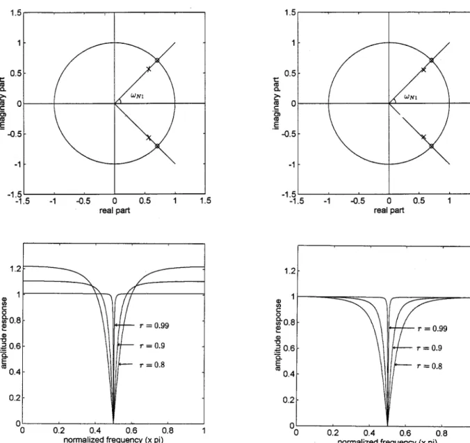
Fig. 1. Type I IIR notch filter. (Top) Pole-zero diagram (x: pole o: zero). (Bottom) Amplitude response for various pole radiusr values.
where is a symmetrical polynomial, that is
Given the notch frequencies , the coef-ficients can be computed by using a recursive relationship developed in [12]. Moreover, poles and zeros of this filter are given by
zeros poles
The zeros are constrained to locate on the unit circle at the notch frequencies , and the poles are at the same radial lines as zeros. Fig. 1 shows the pole-zero diagram and frequency
re-sponse for and notch frequency . For
stability, pole radius must be smaller than one. When ap-proaches unity, the becomes an ideal notch filter.
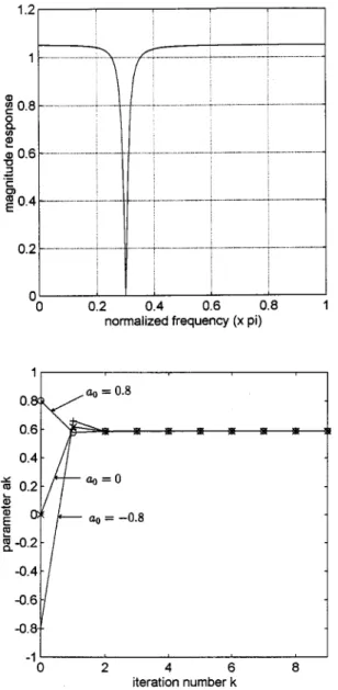
Fig. 2. Type II IIR notch filter. (Top) Pole-zero diagram (x: pole o: zero). (Bottom) Amplitude response for various pole radiusr values.
B. Type II
The transfer function of this type IIR notch filter has the fol-lowing form:
(3) where is a -order allpass filter given by
(4) When notch frequencies are specified, a procedure to de-termine the coefficients is presented in [13]. The zeros of are also at to make the filter a zero gain at notch frequencies. The poles of are all adjacent to the zeros to compensate for the frequency re-sponse to be the unit gain for the non-notch band. Fig. 2 shows the pole-zero diagram and frequency response for , notch
frequency , and allpass filter
(5) It can be shown that the gains at dc and Nyquist frequencies are always equal to unity. When approaches one, the becomes an ideal notch filter.
Based on the above description, a two-stage approach to de-sign the notch filter is as follows.
Step 1) Place zeros on the unit circle with
an-gles . Thus, the
nu-merator of transfer function is equal to .
Step 2) Place poles inside the unit circle and near zeros to make the frequency response of the non-notch band be the unit gain. When poles approach zeros, the notch filter becomes the ideal one. From the above discussion, a question may be asked. What is the optimal pole placement? The pole placements in the type I and II notch filters are just two subjective choices. In this paper, we will use the weighted least squares method to find the op-timal pole locations. Because the stability of single notch filter is easy to control, let us start with the design of single notch filter in Section III.
III. SINGLENOTCHFILTERDESIGN A. Design Method
The general form of transfer function of single notch filter is expressed as
(6) where the numerator and denominator are given by
Let ; then, the poles of this filter are , and the parameter must satisfy the following linear constraint
(7) In our design, the pole radius is specified in advance. Thus, the problem reduces to find the angle such that the cost function
(8) is minimized, where integral region
and is a weighting function. Note that is a pre-scribed small positive number. Substituting (6) into (8), we have
(9)
where and are given by
Using the technique described in [19], the optimization problem in (9) can be solved by the following iterative scheme:
(10)
where , , and are
Real
(11) The notation Real denotes the real part of complex number, and Imag denotes the imaginary part of complex number. Note that the denominator polynomial obtained from the preceding iteration is treated as a part of the weighting function in this scheme. Moreover, at the th iteration,
is known; therefore, the parameter can be determined by solving the standard quadratic programming problem
Minimize
Subject to (12)
Since only single variable is considered in this optimiztion problem and cost function is a parabola with its mouth opened up, the unique closed-form optimal solution is obtained as follows:
if if if
(13)
Based on the above description, we propose an iterative quadratic programming algorithm for obtaining the notch filter coefficent as follows.
Step 1) Specifiy the pole radius , notch frequency , in the integral region , and the weighting function
.
Step 2) Given initial parameter , set .
Step 3) Compute the values , , and using (11).
Step 4) Calculate the quadratic programming solution in (13) to obtain the new coefficient .
Step 5) Terminate the iterative procedure if
(14) where is a preset small positive number. Otherwise, set , and go to step 3.
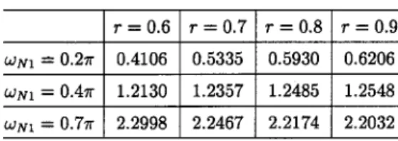
Fig. 3. (Top) Magnitude response of the designed single notch filter. (Bottom) Convergence curves ofa for various initial values a .
B. Design Example
Here, we present one design example of IIR notch filter to demonstrate the effectiveness of the proposed method. The pro-gram is performed in an IBM PC compatible computer (Intel Pentium II CPU insided) using the MATLAB language.
Example 1: In this example, let us consider the following
specifications for the notch filter: • pole radius ;
• notch frequency ;
• ,
• weighting function for all .
The initial parameter is chosen as . When the pro-posed algorithm with is used to design this filter, the resultant magnitude response of this filter is shown in Fig. 3(a). It is clear that the specification is well satisfied. To illustrate the convergence of the algorithm, the values are listed in Table I as a function of the number of iterations. It is seen that the errors
TABLE I PARAMETERa INEXAMPLE1
do not change significantly past three iterations. Thus, conver-gence speed of proposed algorithm is very fast.
In order to illustrate that the convergence of the proposed al-gorithm is insensitive to the choice of initial parameter , the convergence curves of for various initial values are shown Fig. 3(b). Fortunately, all of the curves converges the same final values. Thus, the design algorithm is initially independent. In fact, from an optimization-theoretic viewpoint, (12) is a convex quadratic programming problem that always has a unique min-imizer. This is why the algorithm always converges to the same minimizer, regardless of the initial point used.
C. Discussion
Given notch frequency and pole radius , type I and type II notch filters can be obtained immediately by simple compu-tation, and our method needs to take a lot of time to produce the optimal notch filter. If we care about the design time, we may discard the optimal method and choose heuristic type I or the type II notch filter. Meanwhile, a criterion must be provided to evaluate whether the type I or the type II notch filter is better. One of the methods is to compute the distance between the poles of two types of notch filters and the poles of optimal one because the zeros for the three notch filters are the same. The smaller the distance is, the better the notch filter is. Since three notch filters also have the same pole radius , we only need to compare the pole angles, which are given by
Type I pole angle Type II pole angle Optimal pole angle
Tables II–IV list three pole angles for various notch frequencies , pole radii , and . It is clear that type II is closer to the optimal one than the type I notch filter. Thus, type II is a better choice than type I in this sense.
IV. MULTIPLENOTCHFILTERDESIGN
The general form of the transfer function of IIR multiple notch filter is expressed as
TABLE II
POLEANGLES OF THETYPEI NOTCHFILTER FORVARIOUSNOTCH
FREQUENCIES! ANDPOLERADIUSr
TABLE III
POLEANGLES OF THETYPEII NOTCHFILTER FORVARIOUSNOTCH
FREQUENCIES! ANDPOLERADIUSr
TABLE IV
POLEANGLES OF THEOPTIMALNOTCHFILTER FORVARIOUSNOTCH
FREQUENCIES! ANDPOLERADIUSr
where the numerator is defined in (2), and the denominator is denoted by
(16)
is the pole radius, and are pole angles. The transfer func-tion is a generalization of the conventional type I notch filter. When are chosen as notch frequencies , be-comes the type I notch filter in (2). However, this choice is not optimal. The best choice can be obtained by finding the pole angles to minimize the cost function
(17) Because is not a quadratic function of angles , the quadratic programming approach cannot be applied to solve this nonlinear optimization problem. In order to obtain a satisfactory solution, we rewrite in (16) as follows:
(18)
The coefficients of has the following symmetrical
prop-erty: and .
Define two vectors and
..
. (19)
Then, the polynomial can be rewritten as
(20) Instead of finding pole angles to minimize function , we will find coefficient vector to minimize . Thus, (17) can be rewritten as
(21) where and are given by
and the integral region
. Using the technique developed in [19], the optimization problem in (21) can be solved by the following iterative scheme:
(22) where matrix , vectors , and scalar are
Real
Real (23)
Note that the denominator polynomial obtained from the pre-ceding iteration is treated as part of the weighting function in this scheme. Moreover, at the th iteration, is known; therefore, the parameter can be determined by solving the following optimization problem:
Minimize
Subject to the zeros of are all inside
the unit circle (24)
Because the symmetry of the coefficients is only necessary but not sufficient for all poles to lie on a circle with radius , the
condition does not guarantee that the filter is stable as in the single notch filter case. Thus, the stability problem must be solved by imposing a set of linear constraints on the coefficient of such that all of zeros of are inside the unit circle. Fortunately, Lang has proposed an interesting method to solve this problem [14]. This method is mainly based on Rouché’s theorem.
Rouché’s Theorem: If and are analytic inside and on a closed contour , and on , then and
have the same number of zeros inside .
A proof of Rouché’s theorem can be found in [15]. Now, let the contour be the unit circle, and let the denominator polyno-mial at iteration step have all its zeros inside the unit circle; then, according to Rouché’s theorem, the denomi-nator polynomial in the next iteration is given by
(25) and will also have all its zeros inside unit circle if the following condition is satisfied:
(26) Since two polynomials and are given by
(27) where has been defined in (19) and
(25) can be rewritten as
(28) Substituting (28) into (22), we obtain
(29) where
(30) Next, we study the constraints in (26). Let
be the set of dense grid points on ; then, this constraint, on the set , reduces to
(31)
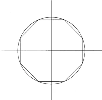
Fig. 4. Approximation of a circle with an octagon.
Letting , the vectors
Real Imag and two scalars
(32) (31) then becomes
(33) Obviously, it is a quadratic constraint of the coefficients . Now, this quadratic constraint can be converted to the linear constraints by approximating a circle with an octagon shown in Fig. 4. This approximation technique has also been used in the design of FIR filters in the complex domain [16]. Thus, the quadratic constraint in (33) can be approximated by the fol-lowing linear constraints:
(34) It is clear that if satisfies the linear constraints in (34) simultaneously, the must satisfy the quadratic constraint in (33). Substituting (32) into (34), we obtain
where matrix and vector are given by
(36) Using matrix notation, the condition in (35) becomes
(37) where
..
. ... (38)
Thus, the problem in (24) can be rewritten as the standard quadratic programming problem as
Minimize
Subject to (39)
Based on the above description, we propose an iterative quadratic programming algorithm for obtaining the denomi-nator polynomial of notch filter as follows.
Step 1) Specify the notch frequencies
, in the integral region , weighting func-tion , number of grid points , pole radius , and parameter .
Step 2) Specify the initial polynomial
. Compute the vector , and set .
Step 3) Use (23) to compute , , and . Step 4) Use (30) to compute , , and . Step 5) Use (36)–(38) to compute the stability constraint
pa-rameters and .
Step 6) Solve the quadratic programming problem in (39) to obtain the coefficient .
Step 7) Compute by using (28), i.e.,
Step 8) Terminate the iterative procedure if
(40) where is a preset positive number. Otherwise, set
, and go to Step 3.
The proposed design algorithm for the multiple IIR notch filter depends on the existence of efficient algorithms to solve
the quadratic programming (QP) problems that have been known for a long time. In the context of FIR filter design, several algorithms for solving the constrained least squares problem have been presented [17], [18]. On the other hand, using the QP to design IIR filter has also been investigated recently [19], [20]. In this paper, the subroutine QP.m in the optimization toolbox of MATLAB software is used to solve QP problem.
In the following, we present two design examples of the IIR multiple notch filter to illustrate the effectiveness of the pro-posed method. One is where distances between notch frequen-cies are large, and the other is where distances are small.
Example 2: In this example, let us consider the following
design parameters for the IIR multiple notch filter:
• notch frequencies , ,
, ;
• pole radius , , , ,
;
• weighting function for all .
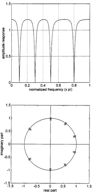
The design algorithm converges after three iterations. The re-sultant amplitude response of this filter and pole-zero diagram is shown in Fig. 5. It is clear that the specification is well satis-fied. Moreover, the square error defined in (21) is 0.5982 for the designed filter, 0.5989 for the conventional type II notch filter, and 0.6002 for the conventional type I notch filter. Thus, our approach provides a smaller design error than the conven-tional methods. Eight poles of the designed notch filter are given in the first expression shown at the bottom of the next page. Clearly, the radii of all poles are equal to the prescribed value 0.95; hence, the filter is stable. From this result, we see that the symmetric condition can make poles lie on a circle with pre-scribed radius if notch frequencies are well separate.
Example 3: The design parameters of this example are same
as those of Example 2, except that the notch frequencies
, , , and , and
the pole radius . That is, we let the notch frequency be very close to . The design algorithm converges after 12 iterations. The resultant amplitude response and pole-zero diagrams are shown in Fig. 6. From this result, we see that the amplitude response is almost equiripple in the non-notch band. The squares error defined in (21) is 2.2029 for the designed filter, 2.3246 for conventional type II notch filter, and 2.8750 for the conventional type I notch filter. Thus, our approach provides smaller design error than the conventional methods. Moreover, eight poles of the designed notch filter are given by the second expression at the bottom of the next page. Clearly, the maximum pole radius is equal to 0.9104; hence, the designed filter is stable. From this result, we see that the symmetric condition can make poles corresponding to well-separate notch frequencies and be on a circle with prescribed radius , but it cannot make poles corresponding to close notch frequencies and be on the prescribed circle. This result is because that symmetric condition is only necessary but is not a sufficient condition. Rouché’s theorem is only used to make those poles corresponding to close notch frequencies be inside the unit circle to guarantee that the filter is stable.
Fig. 5. Design results in the Example 2. (Top) Amplitude response. (Bottom) Pole-zero diagram (x: pole o:zero).
V. CONCLUSIONS
In this paper, a two-stage approach to design stable IIR notch filters has been presented. First, the numerator of the transfer function of the IIR notch filter is obtained by placing the zeros on the unit circle with angles equal to the prescribed notch frequencies. Then, the denominator polynomial is determined by using an iterative scheme in which the optimal pole place-ments are found by solving a standard quadratic programming
Fig. 6. Design results in Example 3. (Top) amplitude response. (Bottom) pole-zero diagram (x: pole o:zero).
problem. For stability, the pole radius in the single notch filter design is specified by the designer, and in the multiple notch filter design, the pole radius is constrained by using the implications of Rouché’s theorem. Examples are included to illustrate the effectiveness of the proposed technique. However, only 1-D notch filters are considered here. Thus, it is interesting to extend this method to the design of 2-D notch filters. This topic will be studied in the future.
REFERENCES
[1] R. Carney, “Design of a digital notch filter with tracking requirements,”
IEEE Trans. Space Electron. Telem., vol. SET-9, pp. 109–114, Dec.
1963.
[2] K. Hirano, S. Nishimura, and S. K. Mitra, “Design of digital notch fil-ters,” IEEE Trans. Circuits Syst., vol. CAS-21, pp. 540–546, July 1974. [3] M. H. Er, “Designing notch filter with controlled null width,” Signal
Process., vol. 24, no. 3, pp. 319–329, Sept. 1991.
[4] G. W. Medlin, “A novel design technique for tuneable notch filters,” in Proc. Int. Symp. Circuits Syst., New Orleans, LA, May 1990, pp. 471–474.
[5] S. C. D. Roy, S. B. Jain, and B. Kumar, “Design of digital FIR notch filters,” Proc. Inst. Elect. Eng.—Vis. Image Signal Process., vol. 141, pp. 334–338, Oct. 1994.
[6] S. B. Jain, B. Kumar, and S. C. D. Roy, “Design of FIR notch filters by using Bernstein polynomials,” Int. J. Circ. Theor. Applicat., vol. 25, pp. 135–139, 1997.
[7] T. H. Yu, S. K. Mitra, and H. Babic, “Design of linear phase FIR notch filters,” Sadhana, vol. 15, pp. 133–155, Nov. 1990.
[8] S. C. Pei and C. C. Tseng, “Two dimensional IIR digital notch filter design,” IEEE Trans. Circuits Syst. II, vol. 41, pp. 227–231, Mar. 1994. [9] S. C. Pei, W. S. Lu, and C. C. Tseng, “Analytical two dimensional IIR notch filter design using outer product expansion,” IEEE Trans. Circuits
Syst. II, vol. 44, pp. 765–768, Sept. 1997.
[10] M. V. Dragosevic and S. S. Stankovic, “An adaptive notch filter with improved tracking properties,” IEEE Trans. Signal Processing, vol. 43, pp. 2068–2078, Sept. 1995.
[11] S. C. Pei and C. C. Tseng, “Elimination of AC intereference in elec-trocardiogram using IIR notch filter with transient suppression,” IEEE
Trans. Biomed. Eng., vol. 42, pp. 1128–1132, Sept. 1995.
[12] T. S. Ng, “Some aspects of an adaptive digital notch filter with con-strained poles and zeros,” IEEE Trans. Acoust., Speech, Signal
Pro-cessing, vol. ASSP-35, pp. 158–161, Feb. 1987.
[13] S. C. Pei and C. C. Tseng, “IIR multiple notch filter design based on allpass filter,” IEEE Trans. Circuits Syst. II, vol. 44, pp. 133–136, Feb. 1997.
[14] M. C. Lang, “Weighted least-squares IIR filter design with arbitrary magnitude and phase responses and specified stability margin,” in
Proc. IEEE Symp. Adv. Digital Filtering Signal Process., Victoria, BC,
Canada, June 1998, pp. 82–86.
[15] R. V. Churchill and J. W. Brown, Complex Variables and
Applica-tions. New York: McGraw-Hill, 1984.
[16] X. Chen and T. W. Parks, “Design of FIR filters in the complex do-main,” IEEE Trans. Acoust., Speech, Signal Processing, vol. ASSP–35, pp. 144–153, Feb. 1987.
[17] M. Lang, I. W. Selesnick, and C. S. Burrus, “Constrained least squares design of 2-D FIR filters,” IEEE Trans. Signal Processing, vol. 44, pp. 1234–1241, May 1996.
[18] J. W. Adams and J. L. Sullivan, “Peak-constrained least-squares opti-mization,” IEEE Trans. Signal Processing, vol. 46, pp. 306–321, Feb. 1998.
[19] W. S. Lu, S. C. Pei, and C. C. Tseng, “A weighted least-squares method for the design of stable 1-D and 2-D IIR digital filters,” IEEE Trans.
Signal Processing, vol. 46, pp. 1–10, Jan. 1998.
[20] J. L. Sullivan and J. W. Adams, “PCLS IIR digital filters with simulta-neous frequency response magnitude and group delay specifications,”
IEEE Trans. Signal Processing, vol. 46, pp. 2853–2861, Nov. 1998.
Chien-Cheng Tseng (S’90–M’95–SM’01) was born in Taipei, Taiwan, R.O.C.,
in 1965. He received the B.S. degree, with honors, from Tatung Institute of Technology, Taipei, in 1988 and the M.S. and Ph.D. degrees from the National Taiwan University, Taipei, in 1990 and 1995, respectively, all in electrical engi-neering.
From 1995 to 1997, he was an Associate Research Engineer with Telecom-munication Laboratories, Chunghwa Telecom Company, Ltd., Taoyuan, Taiwan. He is currently an Associate Professor with the Department of Com-puter and Communication Engineering, National Kaohsiung First University of Science and Technology, Kaohsiung, Taiwan. His research interests include digital signal processing, pattern recognition, and quantum computation.
Soo-Chang Pei (S’71–M’86–SM’89–F’00) was
born in Soo-Auo, Taiwan, R.O.C. in 1949. He received the B.S.E.E. degree from National Taiwan University (NTU), Taipei, Taiwan, in 1970 and the M.S.E.E. and Ph.D. degrees from the University of California, Santa Barbara, in 1972 and 1975, respectively.
He was an Engineering Officer with the Chinese Navy Shipyard from 1970 to 1971. From 1971 to 1975, he was a Research Assistant with the University of California, Santa Barbara. He was Professor and Chairman of the Electrical Engineering Department, Tatung Institute of Technology, Taipei, and NTU from 1981 to 1983 and 1995 to 1998, respectively. He is currently a Professor with the Electrical Engineering Department, NTU. His research interests include digital signal processing, image processing, optical information processing, and laser holography.
Dr. Pei received the National Sun Yet-Sen Academic Achievement Award in Engineering in 1984, the Distinguished Research Award from the National Sci-ence Council from 1990 to 1998, the Outstanding Electrical Engineering Pro-fessor Award from the Chinese Institute of Electrical Engineering in 1998, and the Academic Achievement Award in Engineering from the Ministry of Educa-tion in 1998. He was the President of the Chinese Image Processing and Pattern Recognition Society of Taiwan from 1996 to 1998 and is a member of Eta Kappa Nu and the Optical Society of America.