藉由分享而得的影像還原技術

全文

(1)國立交通大學資訊科學與工程研究所碩士論文. 藉由分享而得的影像還原技術 Image Recovery by using Sharing. 研究生：林憲正指導教授：林志青. 中華民國. 教授. 九十五. 年六月.

(2) 藉由分享而得的影像還原技術 Image Recovery by using Sharing. 研究生：林憲正. Student：Sen-Jen Lin. 指導教授：林志青. Advisor：Ja-Chen Lin. 國立交通大學資訊科學與工程研究所碩士論文. A Thesis Submitted to Institute of Computer Science and Engineering College of Computer Science National Chiao Tung University in partial Fulfillment of the Requirements for the Degree of Master in. Computer Science June 2006 Hsinchu, Taiwan, Republic of China. 中華民國九十五年六月.

(3) 藉由分享而得的影像還原技術研究生：林憲正. 指導教授：林志青博士. 國立交通大學資訊科學與工程研究所. 摘要數位影像在 WWW 的環境中可能會被攻擊者竄改資料，或者在傳輸之中發生傳輸錯誤的情形。在本篇論文中，我們提出三種基於「資訊分享」技術的影像還原方法。在第一個方法之中，我們對每個 8x8 影像區塊進行編碼；其後，只要未被破壞的影像區塊數目大於ㄧ門檻值，我們就可以用它們來把其他已被破壞的影像區塊給還原回來。由於第一種方法若整張影像都被拿掉，則無還原機會，所以我們又提出第二種方法「多張影像交叉還原」技術。對於 n 張編碼後的影像，只要有 t 張影像是未被破壞的，我們就可以利用這 t 張影像來還原其他(n-t)張已被破壞的影像。第三種方法是第二種方法的變形；由於管理者可能希望影像具備自我修復的能力，但又不希望降低影像品質，所以我們的第三種方法以增加儲存空間的方式，對於每張輸入的影像會附加一塊類似雜訊的分存影像，而其功能亦可達到和第二種方法相同的效果。除了上述三種方法外，我們也觀察到視覺密碼學(Visual Cryptography)和利用多項式的影像分享(Image Sharing by Polynomials)各有其優劣點；所以本論文最後提出一個結合此二者的新的分享機制；其分存影像可以依據環境狀況來採用其中一種回復方法。. I.

(4) Image Recovery by using Sharing Student: Sen-Jen Lin. Advisor: Dr. Ja-Chen Lin. Institute of Computer Science and Engineering National Chiao Tung University. Abstract In WWW environment, digital images may be tampered by attackers, or get lost during transmitting. In this thesis, we propose three kinds of image recovery methods, based on sharing techniques. In the first method, the given image is partitioned into 8-by-8 blocks, and we encode each 8-by-8 image block. Later, if the number of the non-attacked blocks is greater than a threshold value, then we can recover all the tampered blocks by using them. Because the first method cannot recover the image if it is deleted completely, we propose the second method which is the cross recovery of multiple images. For n encoded images, if t out of the n images are not-attacked, we can recover the other (n-t) images by the t non-attacked images. The second method is not error-free when each image is embedded with recovery information. The third method is a modification of the second method; and it is for the users who require the images to have cross recovery ability without degrading the images’ qualities. This method appends a noisy shadow image to each input image. Besides the three methods described above, it is also observed that Visual Cryptography and polynomial-style image sharing both have their own advantages and disadvantages. So, this thesis also proposes a novel sharing mechanism combining the two methods. The recovery can be according to the computer resources available at the scene.. II.

(5) ACKNOWLEDGEMENTS I would sincerely thank my advisor, Prof. Ja-Chen Lin of his teaching and instruction. He guided me patiently and kindly during my study of the Master’s degree. Without him, it is impossible for me to complete this thesis. Besides, the whole group of the Computer Vision Laboratory at National Chiao-Tung University gave me much help and suggestion. Thanks are also given to them. Finally, I cordially thank my parents for their wholehearted support to my study. This thesis dedicated to them.. III.

(6) TABLE OF CONTENTS ABSTRACT IN CHINESE .................................................................................. I ABSTRACT IN ENGLISH .....................................................................II ACKNOWLEDGEMENT .................................................................... III TABLE OF CONTENTS....................................................................... IV LIST OF TABLES.................................................................................. VI LIST OF FIGURES ..............................................................................VII. Chapter 1 Introduction .........................................................................1 1.1. Motivation....................................................................................................1. 1.2. Related Works ..............................................................................................3 1.2.1. Literature Review of Secret Sharing................................................4. 1.2.2. Literature Review of Image Hiding .................................................6. 1.2.3. Base Transform ................................................................................7. 1.3. Overview of the Proposed Methods.............................................................9. 1.4. Thesis Organization ...................................................................................11. Chapter 2 Detection and Recovery of Tampered Images .....................................................................................12 2.1. Introduction................................................................................................12. 2.2. The Proposed Method ................................................................................13 2.2.1 The Main Algorithm .........................................................................13 2.2.2 The Verification and Recovery Algorithm ........................................17. 2.3. Experimental Results .................................................................................22. 2.4. Discussion ..................................................................................................27. 2.5. Remark.......................................................................................................29. IV.

(7) Chapter 3 Cross Recovery of Multiple Images..............32 3.1. Introduction................................................................................................32. 3.2. The Proposed Method ................................................................................33 3.2.1 The tool to share n pixels ..................................................................33 3.2.2 The Main Algorithm .........................................................................35. 3.3. Experimental Results .................................................................................40. 3.4. Discussion ..................................................................................................43. 3.5. Extra Topic- a lossless version...................................................................43. Chapter 4 Two-Layer Image Sharing....................................48 4.1. Introduction................................................................................................48. 4.2. A Review of the Basis Matrices [B0] and [B1] .......................................50. 4.3. The Proposed Method ................................................................................54 4.3.1 The main algorithm...........................................................................54 4.3.2 Some supportive algorithms .............................................................58. 4.4. Experimental Results .................................................................................61. 4.5. Concluding discussions..............................................................................66. 4.6. An application............................................................................................68. Chapter 5 Conclusions and Future Works......................69 5.1. Conclusions.................................................................................................69. 5.2. Future Works...............................................................................................70. References..........................................................................................................72 Appendix.............................................................................................................77. V.

(8) LIST OF TABLES Table. 2.1. The performance of restoration ratio by Lin’s method. (a) The number of un-recovered blocks for single-tampered-chunk. (b) The number of un-recovered blocks for spread-tampered blocks. ...........................................28 Table 4.1: A comparison between VC and PSS. ..........................................................49. VI.

(9) LIST OF FIGURES Fig. 1.1. The course of pre-processing, tampering and recovering an image. ...............2 Fig. 1.2. An example to change the base of a digital stream from 5 to 7. (a) base-5 look up table. (b) base-7 look up table. ............................................................8 Fig. 1.3. The framework of this thesis. ........................................................................11 Fig. 2.1. The flow chart of the embedding procedure..................................................13 Fig. 2.2. The bit plane of the block B’ .........................................................................17 Fig. 2.3. The flow chart of the verification procedure. ................................................19 Fig. 2.4. The flow chart of the recovery procedure......................................................22 Fig. 2.5. (a) the host image, (b) the stego image (PSNR=40.61 d.b.), (c) a tampered version, (d) the verification image, (e) the recovered image (PSNR=38.71 d.b.). ..........................................................................................................................24 Fig. 2.6. (a) the host image, (b) the stego image (PSNR=37.14 d.b.), (c) a tampered version, (d) the verification image, (e) the recovered image (PSNR=34.72 d.b.). ..........................................................................................................................25 Fig. 2.7. (a) the host image, (b) the stego image (PSNR=37.15 d.b.), (c) a tampered version, (d) the verification image, (e) the recovered image (PSNR=34.33 d.b.). ..........................................................................................................................26 Fig. 3.1. The flowchart of the sharing/revealing phase................................................34 Fig. 3.2. The main algorithm. ......................................................................................37 Fig. 3.3. The recovery algorithm. ................................................................................39 Fig. 3.4. (3, 4) sharing scheme by our method. (a) PSNR = 46.34 db (b) PSNR=46.36 db (c) PSNR=46.37 db (d) PSNR=46.37 db....................................................41 Fig. 3.5. (4, 6) sharing scheme by our method. (a) PSNR = 42.03 db. (b) PSNR = 42.11 db. (c) PSNR = 42.10 db. (d) PSNR = 42.10 db. (e) PSNR = 42.12 db. (f) PSNR = 42.09 db. ............................................................................................42 Fig. 3.5. The encoding algorithm.................................................................................45 Fig. 3.6. (2, 4) sharing scheme by our method. ...........................................................47 Fig. 4.1. A secret image Lena (a), and its JPEG-compressed version Lena* whose VII.

(10) PSNR is 39.31 dB (b). .....................................................................................62 Fig. 4.2. The halftone version (the binary image H) of Fig. 4.1(a)..............................63 Fig. 4.3. The n=4 transparencies T0-T3 generated from the pair {Fig. 4.1(b), Fig. 4.2} in our (t=2, n=4) threshold scheme. .................................................................63 Fig. 4.4. Stacking “any” two transparencies (e.g. 1st and 3rd transparencies here) yield an enlarged binary image of Lena....................................................................64 Fig. 4.5. The gray-value image Lena* (identical to Fig. 4.1(b)) reconstructed using the information embedded in any two transparencies (the 1st and 3rd transparencies here). ..............................................................................................................64 Fig. 4.6. The second experiment. ((t, n) = (3, 4), and this experiment uses 2-by-3 blocks). (a): a secret image Jet. (b): the JPEG-compressed version Jet* whose PSNR is 47.6dB. (c): the halftone version H of Fig. 4.6(a). (d): stacking result using “any three” of the four generated transparencies (here, 1st, 2nd and 4th transparencies). (e): the Jet* (identical to Fig. 4.6(b)) reconstructed using the information embedded earlier in the three transparencies mentioned in Fig. 4.6(d)................................................................................................................65. VIII.

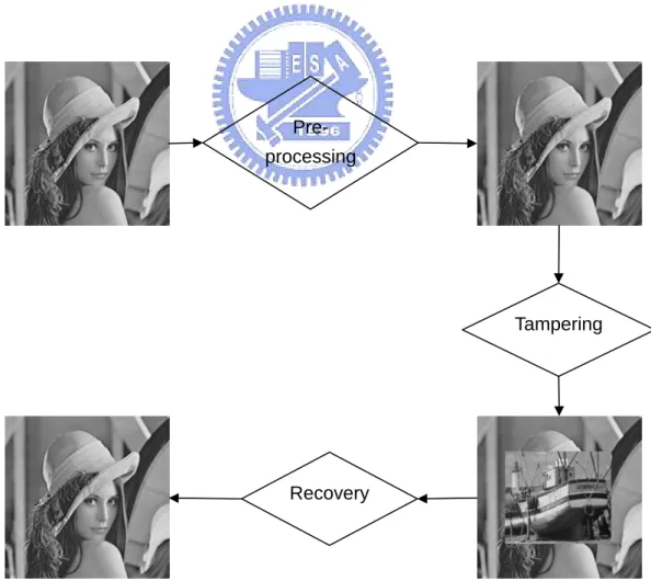
(11) Chapter 1 Introduction 1.1 Motivation Due to the popularity of Internet, people can exchange information conveniently. Many images are placed on Web pages, and authorized people can download them. Unfortunately, it’s hard to ensure that received data is identical to the original data; because Internet is an open environment, anyone can access the data, including attackers. Therefore, how to protect Internet data is a critical issue. In the thesis, we proposed some recovery methods to protect images. Those methods are based on the polynomial sharing technology. This technology contains two phases: the sharing phase and the revealing phase. In sharing phase, the given data are divided into n shadows; later, if anyone get any t of the n shadows (t is a given threshold value), then he can reconstruct the data; but if he gets t-1 or fewer shadows, he can’t get any information about the data. This is a very useful tool for image processing; in recent years, many literatures about this topic have been published [5-22]. With Fig. 1.1, we can realize the procedure of how to recover a tampered image. We roughly separate the process into three parts; the pre-processing step, the tampering step, and the recovery step. For these steps, the pre-processing step and the 1.

(12) recovery step are done by us. How. ever, the tampering is done by the attacker. Thus,. how to design a good algorithm in the pre-processing step and the recovery step is our concern. In Chapter 2, we present a method that can recover a single embedded image based on sharing technology. Since the ability of single image recovery technology is very limited, we also present in Chapter 3 a novel image recovery method for multiple images, and this method can recover the tampered images, even some of the images are destroyed completely.. Preprocessing. Tampering. Recovery. Fig. 1.1. The course of pre-processing, tampering and recovering an image.. 2.

(13) Visual Cryptography was introduced by Naor and Shamir. In (t, n) sharing, the secret data are dispersed into n transparencies, and we can’t get any message about the secret data from each transparency (except for the transparency size). If we stack any t out of n transparencies, then we can “see” the secret message; however, if we stack t-1 or fewer transparencies, then we can’t get any message about the secret data. Some comparisons between polynomial-style secret sharing and Visual Cryptography are described in Chapter 4. Each of the two technologies has its own advantage, thus, we try to combine VC with polynomial-style secret sharing in Chapter 4. Certain transparencies are generated by our method there. If the transparencies can be transmitted via network, the revealing mechanism can get a high quality image (by polynomial-style sharing) with the aid of a computer. But if there is a no computer, then, we still can get “view” a rough look of the secret image by stacking the transparencies.. 1.2 Related Works In this section, some previous works about Secret Sharing and Image Hiding technology will be reviewed. In Section 1.2.1, Shamir’s secret sharing method [1], Thien and Lin’s image sharing algorithm [7] and Galois field will be described briefly. In Section 1.2.2, we will introduce a simple method to hide a base-k digit stream in a. 3.

(14) host image. Because base transform is commonly used repeatedly in this thesis, it is also reviewed in Section 1.2.3.. 1.2.1 Review of Secret Sharing Sharing technology is one of the commonly used methods to protect secret data. Shamir’s secret sharing [1] is a threshold method based on the polynomial interpolation. The (t, n)-threshold secret sharing scheme can disperse the secret data into n shadows, and each shadow has the properties below: 1.. Any t (or more) out of n shadows can be used to reconstruct the secret data.. 2.. Any t-1 (or fewer) shadows cannot be get any information about the secret data.. The. secret. data. could. be. text. files, images,. multimedia. data,. or. encryption/decryption keys. The polynomial used in Shamir’s method is described below:. Shamir’s (t, n)-threshold secret sharing: For (t, n)-threshold sharing, let. Q( x) = a0 + a1 x + a2 x 2 + ... + at −1 x t −1. 4.

(15) where a0 is the secret data, a1 , a2 ,..., at −1 are random numbers, and the n shadows are {1, Q(1)},{2, Q(2)},...,{n, Q(n)} . Any t-1 or fewer shadows can’t get any useful information about the secret data. However, when people receive any t of those shadows, they can evaluate the secret data a0 by using Lagrange interpolation.. In order to save space, Thien and Lin [7] modify the above idea and apply it to the sharing of secret images. For (t, n)-threshold scheme of secret image sharing, an image f of size L is breaks into n shadows, and each shadow has following properties: 1.. Any t (or more) out of n shadows can be used to reconstruct the secret image.. 2.. The size of each shadow is L/t.. The algorithm is very similar to Shamir’s secret sharing scheme, and we introduce the method below.. (t, n)-threshold Secret Image Sharing:. Steps: 1.. For whole secret image, if a pixel value g is larger than 250, then change the value into 250, and creates one more pixel whose gray value is g-250.. 2.. Encrypt the secret image by a encryption key.. 5.

(16) 3.. Divide the secret image into several sections, each section has t pixels.. 4.. For each section, we define the polynomial P( x) = a0 + a1 x + a2 x 2 + ... + at −1 x t −1 (mod 251) where a0 , a1 ,..., at −1 are t pixels of the section.. 5.. Evaluate Share1 = P(1) , Share 2 = P(2) , ..., Sharen = P(n) . Each Sharei is assigned to each shadow image i.. When we receive any t of those shadow images, we can evaluate the secret pixels by using Lagrange interpolation.. If some pixel values of the secret image are larger than 250, the coding, decoding, and share size will all be influenced a little. A better method is that, we change the finite field of the sharing polynomial, as below: Let Galois field be a finite field, denoted by GF ( p n ) , where p is a prime number, and n is a positive integer. In this thesis, unless stated otherwise, the polynomial sharing technology works on GF (28 ) = GF (256) , rather than GF(251).. 1.2.2 Review of Image Hiding Image hiding is a method to embed some secret data in a cover image. For the same hiding capacity, the goal is usually to reduce the difference between the cover. 6.

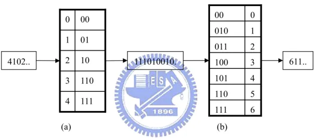
(17) image and the stego image for human’s sense. The simplest hiding method is the least significant bit (LSB) method; the data are embedded in the least k bits of the pixels. In order to improve the image quality of the cover image, Thien and Lin present a method to embed the secret data by using modulo operation [28]. Thien and Lin’s algorithm is more complex than the LSB method; in this thesis, we use a simpler method [30] whose performance is identical to Thien & Lin’s, as below:. Algorithm of module-based data hiding. Let p be a pixel value, d ∈ {0,1,…,b-1} a secret digit to be hidden, and b the module-base. To embed d in p, we replace p by p ' = d + b × rounding[. p−d ] . If p' < 0 , b. then p' ← p'+b . Similarly, if p' > 255 , then p' ← p'−b . Here, the rounding operator means rounding to the “nearest” integer. Also, we assume the pixel value is at least 0 and at most 255. Later, if we want to extract the value d from p′, just use d ← p' (mod b) .. 1.2.3 Base Transform In this thesis, changing the base of a digital stream is a tool used often. We propose a simple method to do this. An example of our method is shown in Fig. 1.2. In this example, we change the base of a digit stream from 5 to 7. The method can be. 7.

(18) divided into two stages. In the first stage, we generate a look up table, as shown in Fig. 1.2(a). This table can map each digit to a binary code. Thus, a binary stream could be yielded. In the second stage, we generate a 7-base look up table, as shown in Fig. 1.2(b). By using the table, we can transform the binary stream into a base-7 digit stream. Later, if we want to convert the digital stream into the original stream, we only reverse this procedure.. 4102... 0. 00. 1. 01. 2. 10. 3. 110. 4. 111. 111010010.. (a). 00. 0. 010. 1. 011. 2. 100. 3. 101. 4. 110. 5. 111. 6. 611... (b). Fig. 1.2. An example to change the base of a digital stream from 5 to 7. (a) base-5 look up table. (b) base-7 look up table. No matter in stages 1 or 2, we need a look up table to map the base from 5(or 7) to 2.. Algorithm of generating a base-k look up table. Input: The base k. Output: A look up table. 8.

(19) Steps: 1.. Evaluate integers c and b so that c = ⎡log 2 k ⎤ and b = 2 c − k .. 2.. For each digit from 0 through b-1, the corresponding binary code is its ...3 00 , 1 → 00 ...3 01 , (c-1)-bit binary expression 0(for example, 0 → 00 12 12 c −1 bits. c −1 bits. 2 → 00 ...3 10 , …). 12 c −1 bits. 3.. Let B denote the (c-1)-bit binary expression of b, then append a zero to the right of B, which is the corresponding binary code of b.. 4.. Each digit from b+1 to k-1 is obtained by adding value to B accordingly.. 1.3 Overview of the Proposed Methods In this section, we will describe the main methods that will be proposed in this thesis briefly. In this thesis, Single-Image Recovery is our first application of the polynomial sharing technology. In the embedding procedure, we use the polynomial sharing technology to share the compressed version (JPEG) of the host image, and then hide each shadow and embed the checksum (CRC64) in each block of the host image. If the image had been tampered, our verification procedure can detect which blocks are altered. Finally, our recover procedure can reconstruct the altered blocks by extracting the compressed version of the original image. However, if the attackers destroy the image completely or replace it with other. 9.

(20) image, the Single Image Recovery technology cannot handle this case. Hence, we propose a Multiple Images Recovery method to resolve the problem. If (n-t) or fewer images of the n images have been deleted, we still can reconstruct those deleted images by the remaining images. Multiple Image Recovery method needs to alter the input images. However, if some people don’t want the images be changed; then they can use a different method of ours to achieve the requirement. The mechanism doesn’t alter any pixel value of the input image, but each image is appended with a shadow file, whose size depends on the threshold value and the size of the input images. Visual Cryptography (VC) is also a secret sharing technology; the most special characteristic of VC is that its is the decoding phase doesn’t need any computer, all we have to do is just to stack those transparencies. Our two-layer Image Sharing method is a method which combines VC with polynomial sharing technology. At the revealing phase, if the decoding-computer is temporarily not available in the decoding sense, we can stack those transparencies to “see” the secret image of rough version. In the other case, when the computer is available, we can get a much finer gray-valued secret image using the information hidden earlier in the shadows by using polynomial sharing algorithm.. 10.

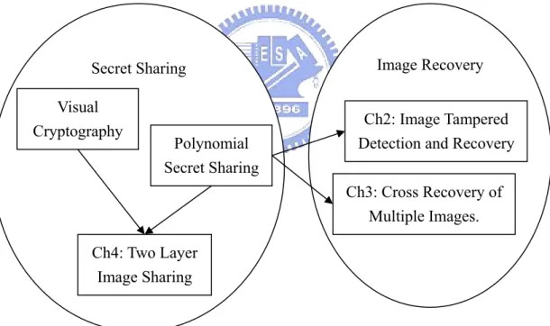
(21) 1.4 Thesis Organization Fig. 1.3 illustrates the framework of this thesis. polynomial secret sharing is the main tool of our whole thesis. In Chapter 2, we will present the scheme of image recovery, which is based on the polynomial sharing approach. The method of cross recovery of multiple images is specified in Chapter 3. Chapter 4 proposes a novel secret sharing method, which can decode the secret image either by a computer or by stacking the transparencies.. Image Recovery. Secret Sharing Visual Cryptography. Ch2: Image Tampered Detection and Recovery. Polynomial Secret Sharing. Ch3: Cross Recovery of Multiple Images. Ch4: Two Layer Image Sharing. Fig. 1.3. The framework of this thesis.. 11.

(22) Chapter 2 Detection and Recovery of Tampered Images This chapter presents an image recovery technology. We use polynomial sharing to share the critical information of the original image into many shadows, and the size of each shadow is very small. Then use data hiding technology to embed those shadows in each block of the original image. Finally, the checksum is also embedded in the block. If the image is tampered, the checksum of each block can determine whether the blocks are altered. If the block is integrity, then the embedded information can be extracted and be used to reconstruct the original image; otherwise, we mark the block as an error block and will be recover by the other integrity blocks.. 2.1 Introduction With the popularity of Internet, we can get multimedia data conveniently. However, attackers can modify those multimedia data easily, via Internet. Therefore, how to protect the integrity of multimedia data is an important issue. Image recovery technology [23-27] is one of the methods to protect important web images. In this chapter, an image recovery method is proposed.. 12.

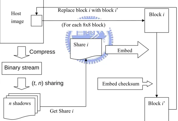
(23) 2.2 The Proposed Method 2.2.1 The Main Algorithm In this section, the host image is a 512-by-512, gray-level image, the range of the gray value is 0~255. Fig. 2.1 shows the embedding procedure of our method.. Replace block i with block i’. Host image. Block i. (For each 8x8 block). Share i Embed. Compress Binary stream. Embed checksum. (t, n) sharing n shadows. Block i’ Get Share i. Fig. 2.1. The flow chart of the embedding procedure. The process of our embedding procedure consists of four stages. The first stage is called “image compression stage”; in this stage, we compress the host image by 13.

(24) using JPEG method (actually, we can use any image compression method). The output is a bit stream, and the resulting size is smaller than the original image file. The second stage is called the “sharing stage”. In this stage, we use polynomial sharing technology to share the binary stream, which was got from the first stage. The final stage is called the “embedding stage”. For each 8-by-8 block, we embed a share and the checksum in it. The details of our method is described in the following algorithm.. Embedding Algorithm: Input: A grey-value host image S of size Width ×Height, a decimal value d, 0＜d＜1,. which indicates the minimal percentage of the integrity blocks needed in order to recover the image if the stego image is tampered later. Output: a stego image. Steps:. 1.. Produce a grey-value image J by compressing the host image S using JPEG compression technology. Hereinafter, the data file representing the compressed image J will be treated as a bit-stream data-file.. 2.. Then, the bit stream of J is shared using an (t, n) sharing algorithm. Where n is equal to the number of 8-by-8 blocks in the host image; that is to say, n= Width/8 ×Height/8. The threshold value t means the percentage of integrity shares could be recovered, so t = d×n. Here the value of n may be 14.

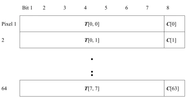
(25) very large; for example, if the image size is 512-by-512, then n=(512/8)×(512/8)=4096, this is a large number. In order to get those shadows, the sharing algorithm must works on GF(212 ) = GF(4096) or modulo 4099(this a minimal prime number which larger than 4096). 3.. Partition the host image S into non-overlapping 8-by-8 blocks, then set i=0 initially. For each 8-by-8 block i, doing following steps.. 4.. Embed the share i was produced at step 2 and a checksum in the block i. The embedding algorithm is described in Embedding-Sub Algorithm. Let the output is a block i’.. 5.. Replace the block i by the block i’, then increment the value of i by 1. Finally, go to Step 4 unless all of the blocks are replaced.. 6.. The image S is our desired output.. Embedding-Sub Algorithm: Purpose: To embed a share data and checksum in an 8-by-8 block. Input: An 8-by-8 block B, and a share data D. Output: An 8-by-8 block B’. Steps:. 1.. Discard all of the least significant bits in the block B. Let T the output block.. 15.

(26) We use a pseudo-code to represent it, For all of pixels in T, T[x, y] ← B[x, y]/2;. Where B[x, y] (resp. T[x, y]) denotes the pixel value at position (x, y) of the block B (resp. block T). 2.. Get the block T’ by using module-based data hiding method (see section 1.2) to hide the share data D in block T.. 3.. Get the checksum C by evaluating the CRC64 of the block T’ (each pixel of the block T’ is consist of 7 bits).. 4.. Append the checksum C to the block T’. Our desired block B’ consists of block T’ and checksum C. We can use the following pseudo-code to get block B’. For all of pixels in B’, B’[x, y] ← T[x, y]+C[x×8+y];. Where C[X] denotes the X-th bit value of the checksum C (C contains 64 bits). Fig. 2.2 shows the bit plane of the block B’.. 16.

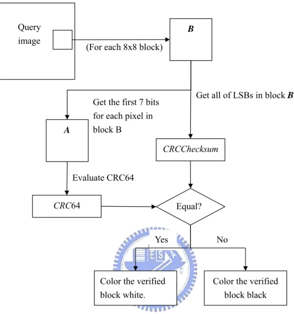
(27) Bit 1. 2. 3. 4. 5. 6. 7. 8. Pixel 1. T[0, 0]. C[0]. 2. T[0, 1]. C[1]. . : 64. T[7, 7]. C[63]. Fig. 2.2. The bit plane of the block B’.. 2.2.2 The Verification and Recovery Algorithm The verification method is based on CRC64. For each 8-by-8 block, we use CRC64 algorithm to check whether the block is integrity or not. If the block is integrity, then we color the corresponding location of the verified image V white; otherwise, color black. The details are described at below.. Verification Algorithm: Input: A query image Q. Output: A verified image V. If a verified block is a black block, it means the block. had been altered. The color is white, if the block is not altered. Steps: 17.

(28) 1.. Divide the query image Q into 8-by-8, non-overlapping blocks.. 2.. For each block B in the image Q, extracting all of LSBs in the block B. Combine those bits, we can get a value called CRCChecksum.. 3.. Evaluating CRC64 of the block B (eliminate all of LSBs in the block B). If the value is equal to CRCChecksum, than we can say this block B is an integral block. Otherwise, the block B is an altered block.. 4.. If the block B is an altered block, we color the block of verified image V black at the corresponding location. Otherwise, color white.. 5.. If there are some blocks un-processed, go to step 2.Otherwise, terminate this procedure, then output the verified image V.. Fig.2.3 illustrates the verification algorithm. With this algorithm, we can know which blocks are tampered. With the verified image, we can even correct those blocks by using recovery algorithm.. 18.

(29) Query image. B. (For each 8x8 block). Get all of LSBs in block B. Get the first 7 bits for each pixel in block B. A. CRCChecksum Evaluate CRC64 CRC64. Equal?. Yes. Color the verified block white.. No. Color the verified block black. Fig. 2.3 The flow chart of the verification procedure. After the image verification procedure, we know which blocks were tampered. In order to recover the tampered blocks, the JPEG version of the original image will be extracted to restore those tampered blocks. The Recovery Algorithm below describes the details of this method.. Recovery Algorithm: 19.

(30) Input: A query image Q and the verified image V. Output: a recovered image R, whose altered blocks had been restored. Steps:. 1.. Divide the image Q into 8-by-8, non-overlapping blocks.. 2.. For each block B, if it is a integral block, extracting the share data which be embedded in the block B.. 3.. Use revealing algorithm to get the secret data from those extracted share files. (The secret data is a JPEG-format file of the original image). From the secret data, we can know a JPEG version of the original image, denote the image is J.. 4.. For each 8-by-8 block of the verified image V, if the block color is black (this means the block had been tampered), we use a corresponding block of the image J to replace the block of the image Q.. 5.. The image Q is our desired output.. Fig. 2.4. Illustrates the three passes of the Recovery Algorithm.. 20.

(31) Pass 1:. Query Image Q. Is it a correct block?. B. Yes Extract No shadow. Verified Image V. Do nothing. Pass 2:. Shadow set. Retrieve the secret data Compressed data of the original image Image decoder. Compressed version of the original image. 21.

(32) Pass 3:. Query Image Q. Verified Image V. JPEG version of the original image. White block. Black block 2 x 1 MUX. Recovered Image R. Fig. 2.4. The flow chart of the recovery procedure.. 2.3 Experimental Results In order to evaluate the ability of our method, in this section, we design some experiments, and the results are show below. 22.

(33) Fig. 2.5. shows our first experiment; Lena is the host image, as shown in Fig. 2.5(a). The decimal value d of embedding algorithm is set 0.5. Fig. 2.5(b) shows the embedded image, which the PSNR is 40.61 d.b.. Fig. 2.5(c) shows that some straight lines had been added on the embedded image. Fig. 2.5(d) and Fig. 2.5(e) show the verification result and the recovered result. The PSNR of Fig. 2.5(e) is 38.71 d.b. (This result is compared with the original image, the following two experiments are also the same). Fig. 2.6. shows our second experiment; Fruit is the host image, as shown in Fig. 2.6(a). The decimal value d of embedding algorithm is 0.25. Fig. 2.6(b) shows the embedded image, which the PSNR is 37.14 d.b.. Fig. 2.6(c) shows some handwriting had been added on the embedded image.. Fig. 2.6(d) and Fig. 2.6(e) show the. verification result and the recovered result. The PSNR of Fig. 2.6(e) is 34.72 d.b.. Fig. 2.7. shows our third experiment; Jet is the host image, as shown in Fig. 2.7(a). The decimal value d of embedding algorithm is 0.25. Fig. 2.7(b) shows the embedded image, which the PSNR is 37.15 d.b.. Fig. 2.7(c) shows a picture “Car” had been added on the embedded image.. Fig. 2.7(d) and Fig. 2.7(e) show the. verification result and the recovered result. The PSNR of Fig. 2.7(e) is 34.33 d.b... 23.

(34) (a). (b). (c). (d). (e) Fig. 2.5. (a) the host image, (b) the stego image (PSNR=40.61 d.b.), (c) a tampered version, (d) the verification image, (e) the recovered image (PSNR=38.71 d.b.) 24.

(35) (a). (b). (c). (d). (e) Fig. 2.6. (a) the host image, (b) the stego image (PSNR=37.14 d.b.), (c) a tampered version, (d) the verification image, (e) the recovered image (PSNR=34.72 d.b.). 25.

(36) (a). (b). (c). (d). (e) Fig. 2.7. (a) the host image, (b) the stego image (PSNR=37.15 d.b.), (c) a tampered version, (d) the verification image, (e) the recovered image (PSNR=34.33 d.b.). 26.

(37) 2.4 Discussion In this chapter, our recovery method is based on polynomial sharing technology. A secret worry is that, if any a mis-judgment occurs in the verification phase, some portions of the image will be lost. Because if any one of the shadows had been altered (or the shadow is a fake), then we cannot get any information at revealing phase! Therefore, the verification phase is very important, we cannot allow any one mis-judgment, and a strict verification algorithm is much needed. Review the verification algorithm of our method, the probability of the correct judgment for a block is 1 − 2 −64 . In our experiment, there are 4096 blocks in a 512-by-512 image. So, the probability of the correct judgment upon all of those blocks is (1 − 2 −64 ) 4096 ≈ 1 − 4096 × 2 −64 = 1 − 2 −52 , this number is very close to 1, so, we can believe that, the case almost doesn’t happen. Lin, Hsieh and Huang [23] present an image recovery method. They use a watermarking technology to embed some recover data in the host image. Table 2.1 shows the relation between restoration performance and the number of un-tampered blocks. From this table, we can know the restoration performance very depend on the ratio of integral blocks to whole blocks. Compare with our method, if the correct blocks is only exceed the threshold, then we can reconstruct the image completely.. 27.

(38) (a). (b) Table. 2.1. The performance of restoration ratio by Lin’s method. (a) The number of un-recovered blocks for single-tampered-chunk. (b) The number of un-recovered blocks for spread-tampered blocks. 28.

(39) 2.5 Remark In our experiment, the number of blocks and the threshold is very large (Actually, in general case, the two numbers should very large). How to increase the speed of encoding/decoding time is a very important issue. Rabin [20] provides a method to design the sharing matrix. For (t, n)-threshold sharing, the time complexity of the revealing phase is θ (t 2 + tL) , where L is the size of the sharing file. However, Rabin’s method requires designing a sharing matrix. This section we introduce a method to compute the inverse matrix, and the time complexity is equal to Rabin’s method. Our method is based on Lagrange’s interpolation. Firstly, the sharing/revealing algorithm will be introduced. We use matrix operator to represent the sharing algorithm. ⎡ h1 ⎤ ⎡10 ⎢h ⎥ ⎢ 0 2 In (t, n) sharing, ⎢ 2 ⎥ = ⎢ ⎢M⎥ ⎢M ⎢ ⎥ ⎢ 0 ⎣hn ⎦ ⎣⎢n. 11 L 1t −1 ⎤ ⎡ s1 ⎤ ⎥⎢ ⎥ 21 L 2 t −1 ⎥ ⎢ s 2 ⎥ , where s1 , s 2 ,..., st are the secret M O M ⎥⎢ M ⎥ ⎥⎢ ⎥ n1 L n t −1 ⎦⎥ ⎣ s t ⎦. message, and h1 , h2 ,..., hn are the n shadows. If we get any t of the n shadows, then we also get the secret message by evaluating the matrix operation below. ⎡ s1 ⎤ ⎡k10 ⎢s ⎥ ⎢ 0 ⎢ 2 ⎥ = ⎢k 2 ⎢M⎥ ⎢M ⎢ ⎥ ⎢ 0 ⎣ st ⎦ ⎣⎢k t. k11 L k1t −1 ⎤ ⎥ k 21 L k 2t −1 ⎥ M O M ⎥ ⎥ k t1 L k tt −1 ⎦⎥. −1. ⎡ hk1 ⎤ ⎢h ⎥ ⎢ k 2 ⎥ , where h , h ,..., h are the t received shadows. k1 k2 kt ⎢ M ⎥ ⎢ ⎥ ⎣⎢ hkt ⎦⎥. 29.

(40) Let L be the size of the secret file, then the time complexity is θ (t 3 + Lt ) , where the term t 3 is the time complexity of computing the inverse matrix. If the threshold t is a large number (In section 2.3, the threshold is 1024 or 2048), the time cost is very much. In order to reduce the time complexity of the revealing algorithm, we proposed a θ (t 2 ) time complexity of evaluating the inverse matrix method. This method is based on Lagrange’s interpolation. Firstly, we rewrite the Lagrange’s interpolation below: t −1. t −1. i =0. j =0 j ≠i. F ( x) = ∑ hki ∏. x−kj ki − k j. t −1. t −1. i =0. j =0. = ∑ hki ∑ bi , j x j. t −1 t −1. t −1 t −1. t −1. t −1. i =0 j =0. j =0 i =0. j =0. i =0. ,. = ∑∑ hki bi , j x j = ∑∑ hki bi , j x j = ∑ x j ∑ hki bi , j. The secret message is the coefficient of the variable x j , so if we use a matrix operation to represent the secret message, then ⎡ s1 ⎤ ⎡ b0,0 ⎢s ⎥ ⎢ b ⎢ 2 ⎥ = ⎢ 0,1 ⎢M⎥ ⎢ M ⎢ ⎥ ⎢ ⎣ st ⎦ ⎣b0,t −1. b1,0 b1,1 M b1,t −1. bt −1,0 ⎤ ⎡ hk1 ⎤ L bt −1,1 ⎥⎥ ⎢⎢hk2 ⎥⎥ , this means bi , j is the coefficient of the O M ⎥⎢ M ⎥ ⎥⎢ ⎥ L bt −1,t −1 ⎦ ⎢⎣ hkt ⎥⎦ L. inverse matrix. Therefore, we can get the inverse matrix by evaluating the polynomial, and the method is described below.. Computing the inverse matrix method: Input: t numbers, i.e. {k i | 1 ≤ i ≤ t}.. 30.

(41) ⎡k10 ⎢ 0 k Output: a t-by-t matrix of ⎢ 2 ⎢M ⎢ 0 ⎢⎣k t. −1. k11 L k1t −1 ⎤ ⎥ k 21 L k 2t −1 ⎥ . M O M ⎥ ⎥ k t1 L k tt −1 ⎥⎦. Notation: ⎡ b0, 0 ⎢b 0 ,1 B=⎢ ⎢ M ⎢ ⎣b0,t −1. b1, 0 b1,1 M b1,t −1. bt −1,0 ⎤ L bt −1,1 ⎥⎥ is the output. i.e., bi , j means the (i+1)th column and O M ⎥ ⎥ L bt −1,t −1 ⎦ L. (j+1)th row of the output matrix. Steps: t −1. 1.. Expand the polynomial G ( x) = ∏ x − k i = g 0 + g1 x + ... + g t −1 x t −1 + x t . i =0. 2.. Let the initial value l be 0.. 3.. Evaluate c = ∏ k l − k j .. t −1. j =0 j ≠l. 4.. Expand. the. polynomial. D ( x) =. G ( x) = d 0 + d1 x + ... + d t −1 x t −1 c( x − k l ). ,. then bl ,0 = d 0 , bl ,1 = d1 ,..., bl ,t −1 = d t −1 . 5.. If value l is t-1, then the matrix B is our desired output; otherwise, go to step 3.. The time complexity of this method is θ (t 2 + t (t + t )) = θ (t 2 ) .. 31.

(42) Chapter 3 Cross Recovery of Multiple Images This chapter presents a novel cross recovery system of multiple images. We use polynomial-sharing and module-based data-hiding techniques to hide the recovery message. If any (n-t) of the n stego images are lost, then the system can recover these stego images by using other t stego images.. 3.1 Introduction In a (distributed) storage system of n images, if some images were lost, a trivial way to recover them is by the back-up copies (identical to the lost images but stored elsewhere). Recently, there are some non-trivial approaches [23-27] that recover a tampered image gorgeously. In this chapter, instead of dealing with a single image, we try to consider several images simultaneously (so that the recovery of any member images in this group can be done through the mutual support of the remaining member images). More specifically, we present a novel cross-recovery method that modify the n input images and obtain n stego images in which the cross-recovery information is hidden; later, up to (n-t) of the stego images are allowed to get lost, for we can still recover the lost stego images using t of the non-lost stego images. Here,. 32.

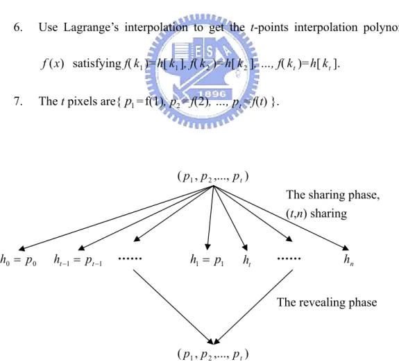
(43) t≧n/2 is a threshold value pre-specified by the reader.. 3.2 The Proposed Method Sec. 3.2.1 presents a novel polynomial sharing method. On basis of this sharing method, our main algorithm is described in Sec. 3.2.2.. 3.2.1 The Tool to Share n Pixels The sharing phase and the revealing phase are described below. Fig. 3.1 shows the flowchart of the sharing/revealing phase. By using the sharing method, the first t shadows is equal to the input message.. The sharing phase: Input: the t pixels. {p i | 1 ≤ i ≤ t }. where 0 ≤ pi ≤ 255 .. Output: n numbers {{h[1], h[2],K , h[t ]}; h[n + 1],K , h[n]} , where 0 ≤ h[i ] ≤ 255 for. each i, and h[1] = p1 , h[2] = p 2 ,K , h[t ] = pt . Steps:. 1.. Use Lagrange’s interpolation (see Ref. [3], the finite Galois Field used here is GF(256)) to get an n-points interpolation polynomial f ( x) satisfying f(1)= p1 , f(2)= p2 , …, f(t)= pt .. 33.

(44) 2.. Compute f(t+1), f(t+2), …, f(n) ; then the u numbers are { {h[1]=f(1)= p1 , h[2]=f(2)= p2 , …, h[t]=f(t)= pt }; h[t+1]=f(t+1),…, h[n]=f(n)}.. The revealing phase: Input: any t of the n shadow-numbers, i.e. {h[k i ] | 1 ≤ i ≤ t} where 1 ≤ k i ≤ n for. each k i . Output: the t pixels {pi | 1 ≤ i ≤ t}. Steps:. 6.. Use Lagrange’s interpolation to get the t-points interpolation polynomial. f (x) satisfying f( k1 )=h[ k1 ], f( k 2 )=h[ k 2 ], …, f( k t )=h[ k t ]. 7.. The t pixels are{ p1 =f(1), p2 =f(2), …, pt =f(t) }.. ( p1 , p 2 ,..., p t ) The sharing phase, (t,n) sharing h0 = p0. ht −1 = pt −1. ……. h1 = p1. ht. ……. hn. The revealing phase. ( p1 , p 2 ,..., p t ) Fig. 3.1. The flowchart of the sharing/revealing phase.. 34.

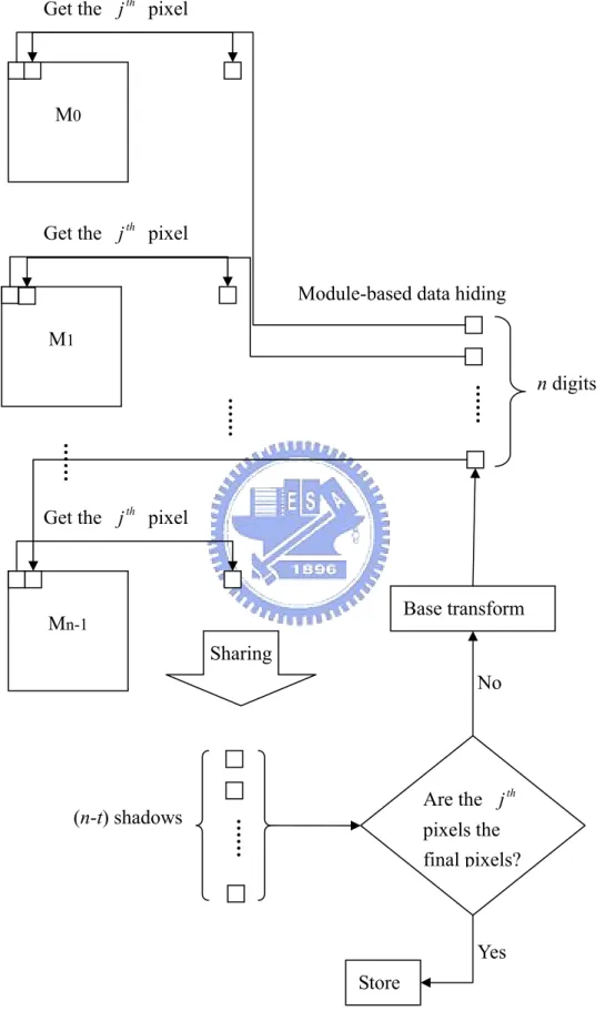
(45) 3.2.2 The Main Algorithm The Main Algorithm: Input: n gray-level images {M i | 1 ≤ i ≤ n} (each is, say, 512-by-512); and a specified. integer t≧n/2. Output: n stego images. Goal: Later, if any (n-t) of the n stego images are lost, we may recover the lost stego. images by using other t stego images. Steps:. 1.. Let the initial value of j be 1.. 2.. Let M i [ j ] denote the j th pixel value of the i th image M i . Then use the sharing tool in Sec. 2.2 to share the n pixel values {pi | 1 ≤ i ≤ n; pi = M i [ j ]} and. thus. generate. u = 2n − t. shadow-numbers. {h[1], h[2],K , h[n],K, h[2n − t ]} . 3.. Among the 2n-t shadow numbers, the final (n-t) shadow-numbers {h[n+1], h[n+2], …, h[2n-k]} are the auxiliary data. In order to hide the auxiliary data. in n images, we need to split the data into n units. Therefore, before hiding, treat these (n-t) numbers (each is in the range 0-255) as a value of (n-t) digits in the base-256 system; then, transform this value from base-256 to a. 35.

(46) n-digits. value. d1d 2 K d n. in. the. base-b. system. (where. b=. n−k ⎤ ⎡ (n-t)/n n 256 ) is the smallest integer not less than 256(n-t)/n). ⎥ =ceiling(256 ⎢ ⎥ ⎢. 4.. For i=1,2,..,n, respectively, hide in M i [ j + 1] the i th digit d i of the base-b auxiliary data. (d1d2 K d n )b. by the module-based data-hiding. algorithm mentioned in Section 1.2.2. 5.. Let j ← j + 1 . Then go to step 2 if j < 512×512=262144 (the image size).. 6.. The images {M i | 1 ≤ i ≤ n} are now the desired output. Also store in a safe place (or attach to each stego image) the n numbers {M i [262144] | 1 ≤ i ≤ n} where 262144=512×512 is the final pixel-position. Use these n numbers as a recovery seed later.. 36.

(47) Get the j th pixel. M0. Get the j th pixel Module-based data hiding M1 ……. ……. ……. Get the j th pixel. Base transform. Mn-1 Sharing. No. pixels the final pixels?. ……. (n-t) shadows. Are the j th. Yes Store. Fig. 3.2. The main algorithm. 37. n digits.

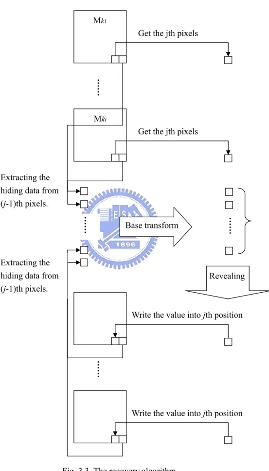
(48) The Recovery Algorithm: Input: t gray level stego images {M ki | 1 ≤ i ≤ t} . Output: n recovered images. Goal: Recover the other (n-t) tampered images by using the input t images. Steps:. 1.. Let the value j be S, where S is one of the size of the input images (each image size is the same value).. 2.. Set the t shadow values are {h[1] = M k1 [ j ], h[2] = M k2 [ j ],..., h[t ] = M kt [ j ]} . Then set {h[t + 1], h[t + 2],..., h[n]} be the store values generated at the main algorithm step 6 (must revealing the base).. 3.. Recover. the. jth. deleted. pixels. by. revealing. the. n. shadows {h[1], h[2],..., h[n]} described in Sec. 3.2.2. Then Decrease the value j by 1. If remain any pixel not to recover (In other words, j>0), then go to step 4, else go to step 5. 4.. Set the t shadow values are {h[1] = M k1 [ j ], h[2] = M k2 [ j ],..., h[t ] = M kt [ j ]} . Then set. {h[t + 1], h[t + 2],..., h[n]}. be. the. hiding. values. embedded. in. the. {M k1 [ j + 1], M k2 [ j + 1],..., M kn [ j + 1]} (must revealing the base). Finally, go to step 3. 5.. The images {M i | 1 ≤ i ≤ n} are now the desired output.. 38.

(49) Mk1 Get the jth pixels. ……. Mkt Get the jth pixels. Extracting the hiding data from (j-1)th pixels.. Extracting the hiding data from (j-1)th pixels.. ……. ……. Base transform. Revealing. Write the value into jth position. ……. Write the value into jth position. Fig. 3.3. The recovery algorithm. 39.

(50) 3.3 Experimental Results Fig. 3.4 shows an experiment using (t, n)=(3, 4). If 4-3=1 of the four 512-by-512 stego images in Fig. 3.4 is lost, we can still recover it by using the other three stego images. Without the loss of generality, assume that stego image M 1 is the one disappears. So, we only have M 2 , M 3 , M 4 , and the 4-numbers seed. {M i [262144] | 1 ≤ i ≤ 4}. mentioned in Step 6. We first use Sec 2.3 to extract the n=4. hidden digits (d1d2…d4)b from the seed, where b=ceiling(256(n-t)/n)=4, then covert (d1d2…d4)b to a value h[5]. Together with h[2]=M2[262143], h[3]=M3[262143], h[4]=M4[262143], we have four h[ti], enough to do inverse sharing to recover the. value M1[262143] (see Sec. 2.2). Then, in next iteration, extract analogously the next n=4 hidden digits (d1d2…d4)b from {Mi [262143]｜1≦i≦4}, and convert (d1d2…d4)b to. a new value of h[5]. Together with h[2]=M2[262142], h[3]=M3[262142], h[4]=M4[262142], we can do inverse sharing to recover M1[262142]. The process. repeats to find all values of M1. The recovered image is exactly the once-lost Fig. 3.4(a). The embedding (to achieve cross-recovery goal) did not give the images big impact; for all four stego images shown in Fig. 3.4 have PSNR about 46.3 db. Fig. 3.5 shows another experiment using (t, n) = (4, 6). If 6-4=2 of the six 512-by-512 stego images in Fig. 3.5 is lost, we can still recover it by using the other four stego images. The six stego images have PSNR around 42 db.. 40.

(51) (a). (b). (c). (d). Fig. 3.4. (3, 4) sharing scheme by our method. (a) PSNR = 46.34 db (b) PSNR=46.36 db (c) PSNR=46.37 db (d) PSNR=46.37 db.. 41.

(52) (a). (b). (c). (d). (e) (f) Fig. 3.5. (4, 6) sharing scheme by our method. (a) PSNR = 42.03 db. (b) PSNR = 42.11 db. (c) PSNR = 42.10 db. (d) PSNR = 42.10 db. (e) PSNR = 42.12 db. (f) PSNR = 42.09 db.. 42.

(53) 3.4 Discussion In this chapter, we have presented a cross recovery system for multiple images. Since we required in the introduction that t≧n/2, i.e. at least one half of the images are not lost, the value of b=ceiling(256(n-t)/n) is at most 16. The p and p′ =d + b×rounding[(p-d) / b] in Sec. 2.2.2 has difference at most 16/2=8 (see Ref. [4]). So the. PSNRs of the stego images are at least 10×log(255×255/(8×8))=30.07 db. (Indeed, our experimental values are about 34 db, when (t, n)=(2, 4) and the four original images utilized to produce Fig. 3.4 are used again as input. ) On the other hand, if t≧3n/4 (the case in Fig. 3.4), then b≧4 and the difference between the input pixel. value p and stego pixel value p′ is at most 4/2=2. The PSNRs of the stego images are therefore at least 10×log(255×255/(4×4))=42.11 db (indeed, the experiment in Fig. 3.4 has PSNRs around 46.3 db).. 3.5 Extra Topic - a Lossless Version The yielded images by the method that be presented in this chapter are loss version images. In this section, we present a loss-less version of image recovery method. However, the dealer must consume extra memory space to store the shadows. Each shadows append to each image, the size of each shadow is depend the original images size and the threshold coefficient.. 43.

(54) The Encoding Algorithm: Input: n gray-value images {M i | 1 ≤ i ≤ n}, and those images are all the same size; and. a specified integer t. Output: n shares, each share consists of a visible image (identical with the input. image) and a shadow. Goal: Later, if any (n-t) of the n image are lost, we may recover the lost images by. using other t images. Steps:. 1.. Use the sharing tool in Sec. 3.2.1 to share the n gray-value images and thus generate 2n − t shadows, then combine those shadows as a large shadow H.. 2.. Use (t, n)-threshold sharing mechanism to share the shadow file H into n sub- shadows {h1 , h2 ,..., hn } .. 3.. For each input image M i , append a sub-shadow hi . Then output those images.. 44.

(55) M1. Share 1. M2. Share 2. ……. ……. Share n. Mn. sharing. (t, n) sharing. h1. h2 …… ……. (n-t) shadow. hn. Fig. 3.5. The encoding algorithm. 45.

(56) If we get any t of the shadow images (or there are (n-t) shadow images have been destroy), then we can recover the miss images by inverse the encoding algorithm. Step 1: Get the secret shadow image H by revealing the noise-like shadow images. Step 2: Recover the images by the revealing algorithm described in Sec. 3.2.1. Actually, because this sharing method can be applied on any binary file, we also can apply this method on any compressed image file (for example, JPEG, JPEG2000,…,etc). The critical advantage is to reduce the memory space of the appended shadow.. Experimental Results Fig. 3.6 shows an experiment in (t, n)=(2, 4). Each input image appends a noise-like shadow image. If 4-2=2 of the four 512-by-512 appended images in Fig. 3.6 is lost, we can still recover it by using the other two appended images. The size of each shadow image is (n/t-1), therefore, if we want the shadow size smaller, the value t must close to n.. 46.

(57) (a). (b). (c). (d) Fig. 3.6. (2, 4) sharing scheme by our method.. 47.

(58) Chapter 4 Two-Layer Image Sharing This chapter presents a novel method to combine two major branches of image sharing: Visual Cryptography and Polynomial-style Sharing. n transparencies are created for a given gray-valued secret image. If the decoding-computer is temporarily not available at (or, not connected to) the decoding scene, we can still physically stack any t received transparencies (t≦n is a threshold value) to get a vague black-and-white view of the secret image immediately. On the other hand, when the decoding-computer is finally available later, then we can get a much finer gray-valued view of the secret image using the information hidden in the transparencies. In summary, each transparency is a two-in-one carrier of the information, and the decoding has two options. The case of virtual-transparencies (electronic-files) is also discussed.. 4.1 Introduction Image sharing can be used in a team when no member alone should be trusted. Visual Cryptography (VC) [1-4] and Polynomial-Style Sharing (PSS) [5-19] are both well-known branches to share images. Both can be designed as (t, n) schemes. (In this. 48.

(59) chapter, we say that a sharing technique is (t, n) if and only if it shares a secret image. S among n shadows so that any t of the n shadows (n≧t) can unveil the secret image S (or a compressed version of S), whereas less than t shadows cannot.) Although both VC and PSS can share images, they are quite different in many manners. The table below compares VC and PSS.. Table 4.1: A comparison between VC and PSS.. The Secret image S being shared. Decoding speed (and decoding method). Visual Cryptography. Polynomial-Style Sharing. Black-and-white. Gray or color. Instant (by using eyes after stacking shadows). Slow (by computation). Is a computer needed in decoding?. No. Yes. Recovered image’s perceptual quality. vague. fine. Size of each shadow. Larger than that of S. Smaller than that of S. From Table 1, we can see that VC is simple and fast, while PSS gives good image quality. A question arises naturally: “Can VC be combined with PSS?” To certain extent, the answer is positive, as is shown here. In this chapter, we present a method to combine these two techniques and achieve a goal: if the decoding-computer is temporarily not available in (or, not connected to) the decoding scene, we can still. 49.

(60) physically stack the t received shadows to get a vague black-and-white view of the secret image immediately; later, when the computer is finally available, we can get a much finer gray-valued view of the secret image using the information hidden earlier in the shadows by using PSS. (In this chapter, our generated “shadows” will be called as “transparencies” because, as mentioned above, one of the two decoding manners is that the shadows can be stacked physically for viewing, just like ordinary transparencies can be stacked and view.) Below in Sec. 4.2 we first review the basis matrices [B0] and [B1] used in VC, and then in Sec. 4.3 we introduce our method. The experimental results are in Sec. 4.4, and the conclusions are in Sec. 4.5. The case that the transparencies are virtual (electronic files) rather than physical is also discussed in Sec. 4.5.. 4.2 A Review of the Basis Matrices [B0] and [B1] Below we review the two basis matrices [B0] and [B1] often mentioned in VC field (e.g. see Reference [2]). The matrix [B0] is called a “white matrix” because it is useful to produce blocks whose stacking result will represent white pixels of a black-and-white (e.g. halftone) image. Matrix [B1] is called a “black matrix” for analogous reason. Without the loss of generality, below we only show the case (t,. 50.

(61) n)=(2,4), i.e. only 2 out of 4 shares are needed in recovering. For a general pair of. given values (t, n), the readers may either design their own [B0] and [B1], or use the appendix to create some pairs of [B0] and [B1] by setting parameters there (see Step 1 of the appendix). In fact, even if the values of u and n are fixed, the choice of [B0] and [B1] is still not unique. To apply the proposed VCPSS two-in-one sharing method, people can use any pair of [B0] and [B1] satisfying the requirements (i)-(iii) stated in next paragraph (these three requirements also appear in the appendix). In summary, the pair [B0] and [B1] is not necessarily generated from the appendix; the appendix is just to let the readers know that there always exists at least one solution to find out [B0] and [B1].. In the (t, n)=(2,4) case, one of the several possible choices for the white matrix [B0] and the black matrix [B1] is to use. ⎡0 ⎢0 [B 0 ] = ⎢ ⎢0 ⎢ ⎣0. 0 0 0 0. 1 1⎤ ⎡0 ⎢1 ⎥ 1 1⎥ ; and [B 1 ] = ⎢ ⎢0 1 1⎥ ⎢ ⎥ 1 1⎦ ⎣1. 0 1. 1 0. 1 0. 1 0. 1⎤ 0 ⎥⎥ . 0⎥ ⎥ 1⎦. (Equation 1). Both matrix has n=4 rows. (In general, no matter how we assign the two matrices, each matrix must have n rows if n transparencies are to be created. This is the so-called requirement (i).) In both matrices, each 0 means that a white element is painted there, and each 1 means a black element is painted there. As we can see, both [B0] and [B1] have 2 black elements per row. (In general, the number of 1s appearing 51.

(62) in each row of [B0] must be identical to that of [B1]. This is the so-called requirement (ii).) It is also obvious that if we stack any two (=t) rows of our [B0], the stacking result has 2 black elements and 2 white elements. On the other hand, if we stack any two(=t) rows of our [B1], the stacking result has at least 3 black elements. (In general, no matter how we choose [B0] and [B1], the number of 1s contained in the result of stacking any t rows of [B1] must exceed that of stacking any t rows of [B0]. This is the so-called requirement (iii).) Now, assume that we want to create 4(=n) blocks, each is 2-by-2 in size, so that stacking any 2(=t) of them will yield a 2-by-2 so-called “white block” (defined here as a block in which only two of the four elements are 1s [i.e. only two black elements]). All we have to do is to permute the columns of [B0] randomly, and then distribute the 4(=n) rows of the permuted [B0] to 4 customers. After that, each customer uses the first two elements as the first row of his block, and next two elements as the 2nd row of his block. As a result, each of the 4(=n) customers has his own 2-by-2 block, and any two of these four 2-by-2 blocks can be stacked to yield a 2-by-2 white block (only two of its 2x2=4 elements are 1s). Similarly, if we want that any t(=2) of the n(=4) created blocks (each is still 2-by-2 in size) can be stacked to yield a so-called “black block” (defined as a 2-by-2 block in which at least three of the four elements are 1s [i.e. at least three black. 52.

(63) elements] ), then we only have to replace the role of [B0] by [B1] in the above argument, and obtain four blocks corresponding to [B1]. Then distribute these four blocks arbitrarily to the four customers (one block per customer.) In the above example, each block has w=2 white elements and b=2 black elements, (or equivalently, each row of [B0] or [B1] has 2 white elements and 2 black elements), and the permutation of the columns of [B0] or [B1] will not affect the stacking result’s brightness (i.e. number of black elements of the stacking result). Moreover, when we do column permutation of the matrix [B0] (or [B1]), if we look at (concentrate on) the first row, we can see that the first row can be either [0011], or [0101], or [1001], or [0110], or [1010], or [1100]. Therefore, all types of row vectors can appear. The by these. C 22 + 2 = C 24 = 6. C bw + b = C 24 = 6 types of blocks represented. C bw + b = C 24 = 6 types of row vectors will be called as fundamental blocks.. (In general, if a VC system uses blocks of size L-by-L, and each block of each transparency has w white elements and b (b=L×L-w) black elements, then there. C bw + b types of fundamental blocks. For example, if 3-by-3 blocks are to be used, and if each block of each transparency has 5 white elements and 4=3x3-5 black elements, then there will have. C 55 + 4 =126 types of fundamental blocks.). As a remark of this section and the appendix, note that the appendix is a self-explained appendix extracted from Ref. [2] which is a graceful paper proposed by. 53.

(64) G. Ateniese et. al. In order to reduce current chapter length and concentrate on our topic, we did not intend to discuss in our appendix the many materials mentioned in Ref. [2]. Interested readers should refer to Ref. [2] for further details. As stated earlier, the appendix here is just to show the readers that they can always create two basis matrices [B0] and [B1] for any pair of given t and n (2≦t≦n).. 4.3 The Proposed Method The n expected transparencies can be created using the main algorithm given below in Section 4.3.1, which is supported by some other supportive algorithms described in Section 4.3.2.. 4.3.1 The Main Algorithm. Main Algorithm (the main algorithm for (t, n) sharing scheme): Input: A grey-value secret image S of size Width ×Height, an integer threshold value t,. and an integer n (n≧t) indicating the number of produced transparencies. Output: n transparencies R = { r0 , r1,..., rn−1} are produced. Steps:. 54.

(65) Step 1. Use the appendix to create two basic matrices [B0] and [B1] for the given t and n (see Sec. 4.2 to understand [B0] and [B1]; see appendix to know. how to create [B0] and [B1].) Then, from the [B0] and [B1], the corresponding values of w and b can be found (each block in each transparency has w white elements and b black elements). Step 2. Since each block of each share is required to have w white elements and b black. elements, there are. C bw + b fundamental blocks. Label all. fundamental blocks, i.e. create a mapping table L that maps each number in {0, 1, …, ( Cbw+ b -1)} to its corresponding fundamental block. Step 3. Produce an image H (the halftone binary version of the image S). Step 4.Produce another grey-value image J=S* by compressing S using some image compression techniques (e.g. JPEG, GIF…); and the compression ratio C must be at least. 8× n so that the space needed to store J is u × log Cbw + b. small enough. Hereinafter, the data file representing the compressed image J will be treated as a bit-stream data-file.. Step 5. Due to security concern, we may encrypt J to get an encrypted bit stream J' . This can either be done by using a security key, or by using some very. simple functions. (For example, to get J', we may just use XOR function in a bit-by-bit manner on the bit stream J and the bit stream of the image H. 55.

(66) (re-read the image H several times if the size of J is larger than that of H). Step 6. Then, the bit stream of J' is shared using an (t, n) sharing method that share a sequence of numbers by polynomials (see Pages 766-767 of Ref. [7]. But we use mod-257 function here to replace the mod-251 function used in Ref. [7] ). Let {s0 , s1 ,..., sn −1} be the n created bit-string-shares. Notably, according to Ref. [7], each bit-string-share is t times smaller than J', so the n so-called bit-string-shares together have n[(Width ×Height × 8 / C)/t] bits.. Step 7. For each si in {s0 , s1 ,..., s n−1} , transform the data in si from base 257 to base. C bw + b . This step is for the hiding purpose later in Step 8. (Because. we only have. C bw + b types of fundamental blocks, we can only embed. digits in the range {0, 1, …, ( Cbw+ b -1)} according to Step 2. ) Step 8. Use the TC Algorithm below to create n transparencies {r0 , r1 ,..., rn −1} so that the n shares {s0 , s1 ,..., s n−1} are hidden in them, and any t of the n transparencies can be stacked to obtain an image looks like the halftone image H. Remark: In Step 4 above, it was stated that the compression ratio (C) must be greater. than. 8× n . We explain why. Since J is the compressed version of S, which has u × log Cbw + b. Width × Height pixels, the number of bits contained in image J (or J') is Width × Height × 8 / C. Then, according to Ref. [TL02], each bit-string-share will have (Width. 56.

(67) ×Height × 8 / C)/t bits after (t, n) sharing of J' by using polynomial-style sharing. Therefore the n bit-string-shares together will have (Width × Height × 8 / C) x n/t bits. On the other hand, since we will use the indices of fundamental blocks to hide the bit-string of each bit-string-share of J' , and since there are. Cbw+b kinds. of. fundamental blocks, each index of a block can represent a value in the range from 0 w+b. through ( Cb. -1). As a result, each block can use its index (the block type) to w+b. recover a value in the range 0~ ( Cb. -1). In other words, if we grab the n so-called. bit-string-shares, and divide their n[(Width × Height × 8 / C)/t] bits into many small segments (each segment has log Cbw+b bits), then each segment can be hidden in (i.e. represented by the block type of) a suitably chosen block whose block index happens to be this value. In summary, the n so-called bit-string-shares can be represented by n[(Width ×Height × 8 / C) /t]/ log Cbw+b blocks. Since S has Width × Height pixels, there are Width × Height binary pixels in H. Since each binary pixel is extended to a block when VC creates transparencies, there will exist Width × Height blocks in the enlarged recovered binary image of H after stacking. So we require n[(Width × Height × 8 / C) /t ] / log Cbw+b ≦ Width × Height .That is why we require C ≧. 8× n . u × log Cbw + b. 4.3.2 Some Supportive Algorithms The main algorithm above requires the use of the following supportive. 57.

(68) algorithms. The TC algorithm is to create n transparencies. The step 2a of this algorithm use a subroutine called TC-SUB. (Notably, TC-SUB is to create n blocks [each transparency will receive one block], and the first of these n blocks can be used w+b. to hide a value in the range {0 ,1,…, ( Cb. -1)}. ). TC Algorithm (Transparencies-creating Algorithm): Purpose: to create n transparencies in which the n shares {s0 , s1 ,..., sn −1} are hidden. Input: the n shares {s0 , s1 ,..., sn −1} , and the halftone image H. Output: n transparencies {r0 , r1 ,..., rn −1} . Steps:. Step1: Divide the halftone image H into n parts of equal size. Then, for each i= 0,1,…,n-1, the Step 2 below will be utilized to hide the encrypted share si with the help of Part i of H. Therefore, set i=0 and j=0 initially, then go to Step 2. Step 2: (To hide the encrypted share si ) (2a): Read the next not-yet-processed integer (the j-th integer si ( j ) ) from the share si ; also read the next not-yet-processed binary pixel (the j-th pixel) value of. Part i of H; then use them to create n blocks {b0 , b1 ,..., bn −1} by the sub-algorithm TC-SUB below. Among {b0 , b1 ,..., bn −1} , the generated block. 58.

(69) b0 is particularly assigned to the transparency ri at location j, and other. n-1 blocks {b1 ,..., bn−1} are arbitrarily assigned to the n-1 remaining transparencies {rl | 0 ≤ l ≤ n − 1, l ≠ i } at location j . (2b): jÅj+1, and go to (2a) unless all integer values { si ( j ) } of si have been processed and embedded in Transparency ri (in that case, go to Step 3 instead). Step 3: Let j=0 again. Increment the value of i by 1. Then go to Step 2 unless i =n. (When i=n, all n shares {s0 , s1 ,..., sn −1} have been hidden in the n transparencies {r0 , r1 ,..., rn −1} .). □. Notably, in the Step (2a) above, si is hidden in ri ; some readers might wonder: at the decoding phase, if. ri is missed, how can si be recovered? To answer this. question, note that si is an (t, n) sharing result (see Step 6 of the Main Algorithm), so any t of n encrypted shares {s0 , s1 ,..., sn −1} can recover the secret information (i.e. the encrypted bit-stream J' of the JPEG image J).. Sub-algorithm TC-SUB Purpose: to hide an integer si ( j ) . Input: an integer value si ( j ) and a pixel q (either black or white) of the halftone. image H.. 59.

(70) Output: n blocks {b0 , b1 ,..., bn−1} (one block per transparency). Notably, the secret. value si ( j ) is hidden in b0 ; meanwhile, stacking together any t of these n blocks can reveal the pixel value (black vs. white) of q. Steps:. Step 1: Use the mapping table L to map the value si ( j ) to a fundamental block. Let b0 be that block. In other words, b0 = L ( si ( j ) ). Step 2: If q is a white pixel, set matrix [B] to the basic matrix [B0] produced in Step 1 of the Main Algorithm. If q is black, set matrix [B] to the basic matrix [B1] .. Step 3: Permute each column of [B] so that the first row of [B] is the same as b0 (treat the 2-by-2 matrix b0 as a row vector of 4 elements). Then, for each d= 1,2,…,n-1, transform Row d of [B] to a 2-by-2 block sequentially assigning the elements of Row d to elements of block Step 4: {b0 , b1 ,..., bn −1} is now the desired output.. bd (by bd ) .. □. Remark (about the TC-SUB algorithm): At the decoding phase, when we stack any t. of the n generated blocks, then, due to Steps 2 and 3 of TC-SUB algorithm, the stacking result will be a black block if and only if the pixel q of the halftone image H is a black pixel.. 60.

(71) 4.4 Experimental Results In our first experiment, the secret image is the image 512-by-512 Lena shown in Fig. 4.1(a). Its JPEG-compressed version, the so-called image J in Step 4 of the main algorithm, is the 512-by-512 Lena* shown in Fig. 4.1(b); and the PSNR of Lena* is 39.31 dB. The 512-by-512 halftone image H of Lena is shown in Fig. 4.2. Assuming (t, n)=(2,4). In other words, the target is that any two of the four generated transparencies can be used for image reconstruction. Then, using Fig. 4.1(b) and Fig. 4.2, the n=4 transparencies are created, as shown in Fig. 4.3. Each transparency is 2×2 times bigger than each image in Fig. 4.1 and .42, for each fundamental block used to expand a pixel (see Sec. 2) is 2-by-2 in this experiment. Now, if we stack any two of the four generated transparencies, as shown in Fig. 4.4, we get a 1024-by-1024 black-and-white image which looks like a 2×2-times enlarged version of the halftone image H shown in Fig. 4.2. On the other hand, if we use the two transparencies to extract the information hidden in them, we can recover exactly the 512-by-512 grey-value compressed image Lena* shown in Fig. 4.1(b), as is shown in Fig. 4.5. In the second experiment, the secret image is the 512-by-512 image “Jet” shown in Fig. 4.6(a). Assuming (t, n)=(3, 4). In other words, the goal is that any three of the four generated transparencies can be used for image reconstruction. The. 61.

(72) corresponding experimental results are shown in the remaining parts of Fig. 4.6. Note that 6(d) is 2-by-3 times larger than the halftone image H because we use 2-by-3 blocks to expand pixels of the halftone image H there. Also note that any two transparencies together (2<3=t) cannot reveal the JPEG version (Jet*) or the halftone version H. (Stacking two transparencies together only gets an image with nothing but noise; no trace of the image H can be seen. As for the reason why the JPEG version Jet* cannot be revealed, it is due to the decoding of Jet* requires the use of the recovered H. [See Steps 1 and 2a of the TC algorithm.]). (a). (b). Fig. 4.1. A secret image Lena (a), and its JPEG-compressed version Lena* whose PSNR is 39.31 dB (b).. 62.

(73) Fig. 4.2: The halftone version (the binary image H) of Fig. 4.1(a).. Fig. 4.3. The n=4 transparencies T0-T3 generated from the pair {Fig. 4.1(b), Fig. 4.2} in our (t=2, n=4) threshold scheme.. 63.

(74) Fig. 4.4. Stacking “any” two transparencies (e.g. 1st and 3rd transparencies here) yield an enlarged binary image of Lena.. Fig. 4.5. The gray-value image Lena* (identical to Fig. 4.1(b)) reconstructed using the information embedded in any two transparencies (the 1st and 3rd transparencies here).. (a). (b). 64. (c).

(75) (d). (e). Fig. 4.6. The second experiment. ((t, n) = (3, 4), and this experiment uses 2-by-3 blocks). (a): a secret image Jet. (b): the JPEG-compressed version Jet* whose PSNR is 47.6dB. (c): the halftone version H of Fig. 4.6(a). (d): stacking result using “any three” of the four generated transparencies (here, 1st, 2nd and 4th transparencies). (e): the Jet* (identical to Fig. 4.6(b)) reconstructed using the information embedded earlier in the three transparencies mentioned in Fig. 4.6(d).. 4.5 Concluding Discussions In this , we have proposed a new method which combines two major branches of. 65.