Stock Returns and Volatility in Emerging Stock Markets
Jaeun Shin*
KDI School of Public Policy and Management, Korea
Abstract
Both parametric and semiparametric GARCH in mean estimations find a positive but insignificant relationship between expected stock returns and volatility in emerging stock markets. The 1997–1998 global emerging market crisis seems to induce changes in GARCH parameters.
Key words: emerging markets; stock returns; volatility; semiparametric GARCH JEL classification: G12; G15; C14
1. Introduction
Understanding the risk-return trade-off is fundamental to equilibrium asset pricing and has been extensively explored in the finance literature. It is perhaps surprising to note, therefore, that there is still much controversy around this important issue. Many traditional asset-pricing models (e.g., Sharpe, 1964; Merton, 1980) postulate a positive relationship between a stock portfolio’s expected return and the conditional variance as a proxy for risk. However, as demonstrated in Campbell (1993), such a positive relationship is contingent on strong assumptions of earlier models. Under more general assumptions, a positive relationship between a stock portfolio’s expected return and the conditional variance may not necessarily apply. More recent theoretical works (Whitelaw, 2000; Bekaert and Wu, 2000; Wu, 2001) consistently assert that stock market volatility should be negatively correlated with stock returns. Obviously, there is no theoretical agreement over the issue.
Empirical studies on the relationship between expected returns and conditional volatility also yield mixed findings. Most of these studies focus on developed markets, particularly the U.S. stock market, and typically employ the parametric (G)ARCH in mean (GARCH-M) model of Engle et al. (1987) to allow for time-varying behavior of volatility. Although some earlier studies (e.g., French et al., 1987) find a positive and significant relationship, more studies (e.g., Baillie and DeGennaro, 1990; Theodossiou and Lee, 1995) report a positive but insignificant
Received December 27, 2004, revised March 15, 2005, accepted March 30, 2005.
*Correspondence to: KDI School of Public Policy and Management, 207-43 Cheongnyangri2-dong,
Dongdaemoon-gu, Seoul 130-868, Korea. E-mail: [email protected]. The author thanks Qi Li and Jian Yang for superb research support.
relationship. Furthermore, consistent with the asymmetric volatility argument, many researchers (Nelson, 1991; Glosten et al., 1993; Bekaert and Wu, 2000; Wu, 2001; Brandt and Kang, 2003; Li et al., 2003) recently report a negative and often significant relationship.
The issue of a proper functional form in modeling conditional volatility has been controversial in this line of research. In particular, many previous studies (e.g., Baillie and DeGennaro, 1990; Theodossiou and Lee, 1995; Choudhry, 1996) are concerned about the appropriateness of modeling conditional variance as a parametric GARCH process and attribute the finding of the weak relationship to the lack of a proper measure of conditional variance. As pointed out by Pagan and Schwert (1990, p. 284-288), the nonparametric estimates of conditional variance adapt more quickly than the parametric (G)ARCH estimates to the fast increase in volatility and to its decrease when a financial panic subsides. The parametric specifications of conditional variance show slow adjustment to large volatility shocks and thus persistent effects of these shocks because these models are only able to capture the persistent, smoother aspects of the data by construction (p. 288). Such a possibility of misspecification in parametric GARCH modeling becomes notoriously serious in the context of GARCH-M estimation because consistent estimation of the GARCH-M model critically depends on correct specification of the full model (Bollerslev et al., 1992, p. 14). By contrast, consistent parameter estimates of the conditional variance equation can still be obtained even in the presence of misspecification in conditional variance in a parametric GARCH model (Bollerslev et al., 1992).
Recently, researchers have empirically demonstrated (e.g., Harvey, 2001; Li et al., 2003) that the relationship between return and volatility depends on the specification of conditional volatility. In particular, using a parametric GARCH-M model, Li et al. (2003) find that a positive but statistically insignificant relationship exists for all the 12 major developed markets. By contrast, using a flexible semiparametric GARCH-M model, they document that a negative relationship prevails in most cases and is significant in 6 out of the 12 markets.
This study comprehensively examines the relationship between expected return and risk in a number of emerging stock markets. Compared to a large empirical literature on developed markets, only a few studies have been conducted on emerging markets, including Choudhry (1996) on 6 emerging markets, De Santis and Imrohoroglu (1997) on 14 emerging markets, and Lee et al. (2001) on China’s stock markets. All these studies are based on a parametric GARCH-M model, and all report positive but not statistically significant relationships between stock market returns and conditional variance in most of the emerging stock markets under investigation.
The main contribution of this study is to present more reliable evidence on the relationship between stock returns and volatility in emerging stock markets by exploiting a recent advance in nonparametric modeling of conditional variance. This study employs both a parametric and a semiparametric GARCH model for the purpose of estimation and inference. The use of a flexible semiparametric
specification of conditional variance is particularly appealing here, as estimation of a parametric GARCH-M model is very sensitive to model misspecification. Very little was previously known about the infinite sample properties of such nonparametric techniques (Bollerslev et al., 1992, p. 13), which might explain why nonparametric modeling of the conditional variance was not widely used. Recently, Batagi and Li (2001) demonstrate the asymptotic normality of a nonparametric estimator of conditional variance as proposed by Pagan and Ullah (1988), which is applicable to the semiparametric estimator used in this paper (see Li et al. (2003) for more details).
The problem that inferences drawn on the basis of GARCH-M models may be highly susceptible to model misspecification is also well known to applied researchers. For example, Jones et al. (1998) do not estimate a GARCH-M model to measure a possible change in the risk premium simply due to the concern that a potential misspecification problem may contaminate the estimation of conditional variance parameters. This study also extends the literature (e.g., Choudhry, 1996; De Santis and Imrohoroglu, 1997) by investigating how the recent 1997–1998 global emerging market crisis might affect the relationship between stock market returns and the conditional variance as well as market volatility.
The rest of this paper is organized as follows. Section 2 briefly discusses the empirical methodology, Section 3 presents empirical results, and Section 4 concludes.
2. Empirical Methodology
This section presents a brief review of the empirical methodology used in this study. To examine the relationship between stock market returns and volatility, both parametric and semiparametric GARCH-M specifications are used.
2.1 A parametric GARCH-M specification
The time varying pattern of stock market volatility has been widely recognized and modeled as conditional variance in a parametric GARCH framework. To be comparable with previous studies on emerging stock markets (e.g., Choudhry, 1996; De Santis and Imrohoroglu, 1997), the parametric method in this study is based on an AR(1)-GARCH (1,1)-M model specified as follows:
t t t t by y =µ+ − +δσ2+ε 1 (1) ) , 0 ( ~ 2 1 t t t N σ ε Ω− (2) 2 1 1 2 1 1 2 − − + + = t t t ω αε βσ σ , (3)
where yt is the stock market return, or the first difference of log stock market index
prices, and ε stands for a Gaussian innovation with zero mean and a time-varying t
conditional variance 2
t
σ . Among the parameters to be estimated, the most relevant one for this study is the parameter δ , because both the sign and significance of this parameter directly shed light on the nature of the relationship between stock market
returns and volatility. More precisely, a significant positive estimate of δ implies that investors who trade stocks are compensated with higher returns for bearing higher levels of risk. A significant negative estimate indicates that investors are penalized for bearing higher levels of risk.
To guard against the possibility that a parametric GARCH-M model may be misspecified, I use a recently developed model specification test to check the correctness of a GARCH specification. Specifically, Hsiao and Li (2001) propose a consistent test for a parametric conditional heteroskedasticity functional form, which can be applied to a time-series regression with weakly dependent data. In light of consistency, this new test outperforms many of the existing tests because, under certain forms of conditional heteroskedasticity, existing tests have only trivial power asymptotically. Hsiao and Li (2001) show that under the null hypothesis of the correctly specified conditional heteroskedasticity, the test statistic they developed follows an asymptotically normal distribution. See Hsiao and Li (2001) for more technical details.
2.2 A semiparametric GARCH-M specification
This study also considers a semiparametric GARCH-M model defined by:
t t t t t t y u x u y =α +α − +δσ + ≡ α+ 2 1 1 0 , (4)
where yt is the stock market return, (1, , )
2 1 t t t y x = − σ , α =(α0,α1,δ)' , and ) var( 1 2 − Ω = t t t y
σ is the variance of yt conditional on Ωt−1 (with Ωt−1 the
information set available at time t−1 ). Consider the following simple semiparametric GARCH model (with var( 1) var( 1)
2 − − = Ω Ω = t t t t t y u σ ): 2 1 1 2 ( ) − − + = t t t mu γσ σ , (5)
where the functional form of m( )⋅ is unspecified. If 2 1 1)
(ut− = + ut−
m α β , then (5) reduces to a standard GARCH(1,1) model. Thus, the semiparametric model (5) contains the parametric GARCH(1,1) model as a special case.
The objective is to assess whether the conditional variance affects the conditional mean of the stock returns. Thus, it is necessary to test the null hypothesis
0
H : δ =0. Under H0 and from (4), one obtains ut−1= yt−1−α0−α1yt−2. A more
general conditional variance specification is:
2 2 2 1 1 2 var( ) ( , ) − − − − = + Ω = t t t t t t y g y y γσ σ , (6)
where the functional form of g( )⋅ is not specified. When g(yt−1,yt−2)= )
( ) (yt−1− 0− 1yt−2 =mut−1
m α α , (6) reduces to (5). Thus, (6) is more general than (5) and allows the conditional variance to have general interactions between yt−s and
1 ( 1, 2,...)
t s
y− − s= .
Next 2
t
σ is estimated based on a recursive version of (6) using the nonparametric series estimation method. See Li et al. (2003) for a detailed
illustration of the estimation procedure. Once ˆ2
t
σ , the resulting nonparametric series estimator of 2 t σ , is obtained, replacing 2 t σ by ˆ2 t σ in Equation (4) yields t t t t y y =α +α − +δσ +ε 2 1 1 0 ˆ , (7) where ( 2 ˆ2) t t t t u δ σ σ
ε = + − . The coefficient vector α =(α0,α1,δ)' is estimated by
least squares, regressing yt on the vector (1, , ˆ )
2
1 t
t
y− σ . Equation (7) contains a
nonparametrically generated regressor, ˆ2
t
σ , and the asymptotic distributional properties of model (7) are worked out by Baltagi and Li (2001).
3. Empirical Results
The data for this study cover 14 relatively well-established emerging markets which have stock price index series available from the International Finance Corporation (IFC) Emerging Markets database. These emerging markets are the same as those studied in De Santis and Imrohoroglu (1997). Regionally speaking, there are 6 Latin American emerging markets (Argentina, Brazil, Chile, Colombia, Mexico, and Venezuela), 6 Asian emerging markets (India, Korea, Malaysia, Philippines, Taiwan, and Thailand), and two European emerging markets (Turkey and Greece). The sample period is from January 1989 to May 2003, after the 1987 international stock market crash. Similar to De Santis and Imrohoroglu (1997), daily data are converted into weekly observations to address the potential autocorrelation problem, yielding a total of 750 weekly observations. All data are in local currency terms.
The data selection of this study has two main advantages. The application of the weekly data instead of the monthly data makes findings of this study directly comparable to those of De Santis and Imrohoroglu (1997). Thus, employing a semiparametric model to this database is expected to provide more reliable evidence for the previous parametric results on the relationship between stock returns and volatility with little concern about the misspecification problem and possible influence of data frequency on results. By including in the sample period observations as recent as May 2003, this study examines the impact of the 1997– 1998 global emerging stock market crisis on GARCH parameters in line with Choudhry (1996), who studies the impact of the 1987 stock market crash using monthly data between January 1976 and August 1994.
Estimation with monthly data tends to reflect long-term movements in volatility by providing the advantage of covering a longer period (Baillie and DeGennaro, 1994, p. 211). As a consequence, the size and significance of parameters in the conditional variance process are expected to depend on data frequency: the GARCH parameter, denoted α in Equation (3), takes values larger in magnitude when 1
monthly data is used if the impact of shocks on the conditional variance gets amplified over time. It reflects higher volatility clustering in the long-run than in the short-run. In this case, it is noted that estimation with monthly data may capture the long-term effect of the stock market shock on volatility. Note that (the
autocorrelation parameter) β , the coefficient in the conditional variance equation, 1
might be larger when using weekly as opposed to monthly data. The autocorrelation in the volatility is stronger in the weekly series (short-run with less noise) than in the monthly series (long-run with more noise), which comes as no surprise. Higher autocorrelation means better predictability of future volatility using past observations. Finally, the persistence of the conditional variance process measured by α1+β1 depends on the relative difference in the sizes of the two parameters
between the weekly series and the monthly series. These conjectures are well verified by findings of this study in comparison with Choudhry (1996, pp. 974-976).
Even though there are some differences in the parameter estimates of the conditional variance process resulting from data frequency choice and even though the monthly data set seems to capture the long-term effect of shocks and autocorrelation of the volatility, I find no particular reason for the major conclusions of this study to be subject to data frequency in any significant way. In fact, empirical results of this study are found to be consistent with previous research that uses monthly data.
The sample period covers “the first truly global emerging market crisis” (Kamin, 1999, p. 506), i.e., the period 1997 to 1998. Both the Asian and the Russian financial crises were major events reflecting the prolonged global emerging market crisis. The literature (e.g., Forbes and Rigobon, 2002) typically defines the window of the Asian financial crisis from October 1997 to November 1997 and the Russian financial crisis from August 1998 to October 1998. Although it is generally hard to precisely define the onset of these crises, the modest variation in the definition of crisis periods does not appear to affect the main findings of this study. There were also other, smaller, and more country-specific crises in the Latin American region during the sample period (e.g., the Brazilian crisis in January 1999). One might treat these events as part of “normal life” in emerging stock markets. Hence, to comprehensively investigate the impact of the 1997–1998 global emerging market crisis on stock volatility and the relationship between stock returns and volatility in these stock markets, I conduct analyses for sub-periods conservatively defined as follows: pre-crisis period (January 1989–June 1997) and post-crisis period (February 1999–May 2003 for Latin America and January 1998–May 2003 for Asia and Europe).
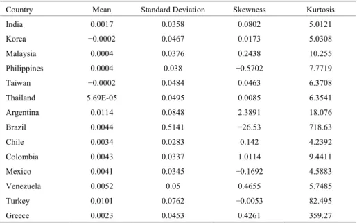
The stock return used in this study is defined as the first difference of the logarithm of stock index prices ( yt =ln(pt pt−1)). Table 1 provides some basic
summary statistics. Because risk-free interest rates were not available to all the emerging markets under consideration during the entire sample period, I use stock returns instead of excess stock returns to conduct analysis. Many researchers (Baillie and DeGennaro, 1990; Nelson, 1991; Choudhry, 1996) show that using stock returns instead of excess returns produces little difference in estimation and inference in this line of research.
Table 1. Summary Statistics for Weekly Stock Returns
Country Mean Standard Deviation Skewness Kurtosis
India 0.0017 0.0358 0.0802 5.0121 Korea −0.0002 0.0467 0.0173 5.0308 Malaysia 0.0004 0.0376 0.2438 10.255 Philippines 0.0004 0.038 −0.5702 7.7719 Taiwan −0.0002 0.0484 0.0463 6.3708 Thailand 5.69E-05 0.0495 0.0085 6.3541 Argentina 0.0114 0.0848 2.3891 18.076 Brazil 0.0044 0.5141 −26.53 718.63 Chile 0.0034 0.0283 0.142 4.2392 Colombia 0.0043 0.0337 1.0114 9.4411 Mexico 0.0041 0.0345 −0.1692 4.5883 Venezuela 0.0052 0.05 0.4655 5.7485 Turkey 0.0101 0.0762 −0.0053 82.495 Greece 0.0023 0.0453 0.4261 359.27
Notes: The indices of skewness and kurtosis for the normal distribution are equal to zero and three, respectively.
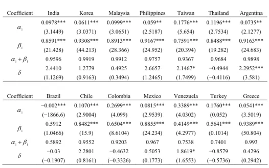
Panels A, B, and C in Table 2 present the results for the most relevant parameters (α , 1 β , and δ ) obtained from the parametric GARCH (1,1)-M tests for 1
the entire period, the pre-crisis period, and the post-crisis period, respectively. Results from the whole period (Panel A) show that the GARCH effect is present for all 14 markets. This is evidence of significant volatility clustering in the stock returns of these markets during 1989–2003. The sum of the GARCH parameters (α1+β1) is often close to unity, implying that volatility shocks are highly persistent
in emerging markets.
Based on the whole sample period, the influence of volatility on stock returns (δ ) is found to be positive for 10 out of 14 markets. A positive time-varying risk premium is significant for 3 markets (Taiwan, Argentina, and Venezuela). Further results based on sub-period analyses suggest a similar pattern. In particular, this influence of volatility on returns is positive for 10 out of 14 markets and a significant positive relationship only exists for Argentina in the pre-crisis period. In the post-crisis period, I find stronger evidence for the significance of the risk premium effect on returns, as the relationship is significant for 4 markets. This implies that the global emerging crisis generates the effect of a risk premium on the stock returns by making investors more alert to market risk. Among these 4 markets, the risk premium is significant and positively correlated with returns for Taiwan, Thailand, and Greece. In contrast, the Brazilian data shows a negative relationship between stock returns and market risk.
Table 2. Parametric GARCH(1,1)-M Estimation Results Panel A: Whole Sample Period
Coefficient India Korea Malaysia Philippines Taiwan Thailand Argentina
1 α 0.0978*** (3.1449) 0.0611*** (3.0371) 0.0999*** (3.0651) 0.059** (2.5187) 0.1776*** (5.654) 0.1196*** (2.7534) 0.0735** (2.1277) 1 β 0.8591*** (21.428) 0.9308*** (44.213) 0.8913*** (28.366) 0.9167*** (24.952) 0.7591*** (20.394) 0.8488*** (19.282) 0.9163*** (24.683) 1 1 β α + 0.9596 0.9919 0.9912 0.9757 0.9367 0.9684 0.9898 δ 2.4410 (1.1269) 1.2779 (0.9163) 0.4925 (0.3494) 2.6657 (1.2465) 2.1467* (1.7499) −0.4944 (−0.4116) 2.2952*** (3.581)
Coefficient Brazil Chile Colombia Mexico Venezuela Turkey Greece
1 α −0.002*** (−1866.6) 0.1070*** (2.9004) 0.2699*** (4.099) 0.0815*** (2.9539) 0.3389*** (4.0302) 0.1760*** (0.052) 0.0541*** (3.5019) 1 β 0.5912 (1.0466) 0.8482*** (15.9) 0.6504*** (8.6104) 0.8855*** (24.234) 0.4149*** (4.2977) 0.5641*** (0.1014) 0.9389*** (50.804) 1 1 β α + 0.5892 0.9552 0.9203 0.967 0.7538 0.7401 0.993 δ −0.03 (−0.1907) 2.2801 (0.8161) −0.4632 (−0.3326) 0.5053 (0.1773) 1.8619* (1.6553) −0.8579 (−0.5736) 0.4296 (0.2942)
Panel B: Pre-Crisis Period
Coefficient India Korea Malaysia Philippines Taiwan Thailand Argentina
1 α 0.1378*** (3.1507) 0.0878 (1.1802) 0.1004** (1.9666) 0.0318 (1.5959) 0.2345*** (3.2153) 0.1383* (1.7198) 0.0681* (1.8116) 1 β 0.8111*** (15.075) −0.103 (−0.4029) 0.8593*** (13.126) 0.9468*** (23.53) 0.7185*** (9.8826) 0.7913*** (9.2656) 0.9298*** (26.814) 1 1 β α + 0.9489 −0.0152 0.9597 0.9786 0.953 0.9296 0.9979 δ 0.6137 (0.2667) 31.775 (1.4066) −0.2532 (−0.0739) 0.1895 (0.0475) 0.699 (0.6033) −2.9676 (−1.1818) 1.8818*** (3.2922)
Coefficient Brazil Chile Colombia Mexico Venezuela Turkey Greece
1 α −0.004*** (−2013.0) 0.1444*** (2.4959) 0.3033*** (3.0951) 0.083* (1.806) 0.4408*** (0.1201) 0.2197*** (0.0664) 0.1713*** (0.0543) 1 β 0.599 (1.1148) 0.7505*** (8.8444) 0.6435*** (6.9812) 0.8439*** (10.199) 0.0749 (0.6864) 0.6028*** (0.0967) 0.76*** (0.0482) 1 1 β α + 0.5953 0.8949 0.9468 0.9239 0.5157 0.8225 0.9313 δ −0.216 (−0.5489) 0.8017 (0.1926) 0.5486 (0.3617) 0.3907 (0.0756) 1.0725 (0.7673) −1.9281 (−1.1959) 0.7954 (0.494)
Panel C: Post-Crisis Period
Coefficient India Korea Malaysia Philippines Taiwan Thailand Argentina 1 α 0.0408* (1.9752) 0.0021 (0.768) 0.0249 (1.4532) 0.1638*** (2.6744) 0.0629* (1.9441) 0.1776** (2.4101) 0.0835 (1.4986) 1 β 0.9554*** (33.035) 0.6354*** (4.0975) 0.9725*** (59.302) 0.7707*** (13.265) 0.8110*** (9.0805) 0.6638*** (5.0245) 0.836*** (7.1164) 1 1 β α + 0.9962 0.6375 0.9974 0.8345 0.8739 0.8414 0.9195 δ 6.1601 (1.3162) 635.26 (0.7939) 1.8201 (0.9205) 3.3921 (1.4601) 22.786* (1.7418) 4.8758* (1.6761) 5.897 (1.4276) Coefficient Brazil Chile Colombia Mexico Venezuela Turkey Greece
1 α −0.066*** (−3.9898) 0.0158 (0.8224) 0.3338*** (3.0776) 0.0546* (1.6672) 0.1289** (2.392) 0.1117 (1.0777) 0.0003 (0.0328) 1 β 0.5402*** (7.4463) 0.9797*** (32.16) 0.2534 (1.2472) 0.9418*** (33.577) 0.7752*** (8.9627) 0.1526 (0.435) 1.0101*** (81.543) 1 1 β α + 0.4745 0.9955 0.5872 0.9964 0.9041 0.2643 1.0104 δ −10.999*** (−2.9336) −4.7437 (−0.367) 2.1336 (0.4245) 1.1283 (0.2934) 3.7795 (0.948) 5.7347 (0.7524) 15.266*** (2.9153) Notes: The symbols ***, **, and * denote statistical significance at the 1%, 5%, and 10% levels, respectively; t-ratios are in parentheses.
As a robustness check, I apply the Hsiao and Li (2001) consistent model specification test to test the correctness of the parametric GARCH(1,1)-M specification. The testing results are reported in Table 3, where it can be observed that at the 5% level, the null hypothesis of a parametric GARCH(1,1)-M conditional heteroskedasticity is not rejected for 10 out of 14 markets with the only exceptions of Philippines (after crisis), Mexico (whole sample and before crisis), Turkey (before crisis), and Greece (whole sample and before crisis). Although Hsiao and Li’s (2001) test may still suffer from some finite sample size distortions due to its slow convergence to its asymptotic distribution, the test results are quite reassuring and suggest that the parametric GARCH(1,1)-M is fairly well behaved. To the best of my knowledge, this is the first time evidence based on a statistical test that a GARCH(1,1)-M model adequately captures the GARCH effect of stock returns has been presented. Previous studies typically examine some gross statistics such as skewness and kurtosis, which may capture the effects of higher moments other than GARCH effects. The results also hint that there might be only minor differences between the parametric and the more flexible semiparametric estimation discussed next.
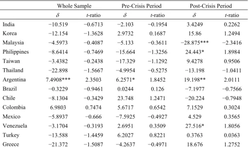
The semiparametric estimation results, as reported in Table 4, to a great extent confirm the findings based on parametric estimation results. Specifically, from Table 3, it can be observed that the estimates of δ are negative in 12 out of 14 markets, which apparently supports the hypothesis of a negative relationship between stock market return and volatility in these stock markets. The only significant relationship
is found for Argentina and is positive at the 1% significance level. However, as shown below, the estimates based on the whole sample period appear to be strongly biased due to ignoring a potential structural change due to the 1997–1998 crisis.
Table 3. Specification Test Results for Parametric GARCH (1,1)-M Model Estimation
India Korea Malaysia Philippines Taiwan Thailand Argentina Whole sample −1.467 0.397 −0.156 −0.999 1.78 −0.923 −0.184 Before crisis −0.702 −0.316 −0.3617 −0.979 −0.22 −0.153 −0.026 After crisis −0.638 −0.66 −2.264 2.23 −1.281 0.226 −2.074 Brazil Chile Colombia Mexico Venezuela Turkey Greece Whole sample −11.62 1.036 0.286 2.159 −0.919 0.93 1.987 Before crisis −9.491 0.369 0.038 2.25 −0.984 2.106 1.974 After crisis −0.973 −1.043 0.855 0.599 0.268 −0.972 −1.441
Table 4. Semiparametric GARCH(1,1)-M Estimation Results
Whole Sample Pre-Crisis Period Post-Crisis Period
δ t-ratio δ t-ratio δ t-ratio
India −10.519 −0.6713 −2.103 −0.1954 3.4249 0.2262 Korea −12.154 −1.3628 2.9732 0.1687 15.86 1.2494 Malaysia −4.5973 −0.4087 −5.133 −0.3611 −28.875*** −2.3416 Philippines −8.6414 −0.7469 −15.664 −1.3256 24.443* 1.8984 Taiwan −3.4382 −0.2438 −17.329 −1.1292 9.4278 0.9506 Thailand −22.898 −1.5667 −4.9954 −0.5275 −13.198 −1.0411 Argentina 7.4908*** 2.3503 6.2571* 1.8452 19.198** 2.0111 Brazil −0.3229 −0.9461 0.0244 0.126 −7.1977 −0.7566 Chile −8.1304 −0.3429 23.748 1.2471 −20.224 −0.7948 Colombia 6.9803 0.7474 5.6717 0.6542 7.1529 0.3024 Mexico −5.8937 −0.666 −7.5925 −0.4927 4.529 0.3565 Venezuela −3.1704 −0.3193 2.6951 0.3509 27.516* 1.8056 Turkey −13.588 −1.4459 6.2027 0.8221 0.3763 0.0363 Greece −21.372 −1.5087 −4.2637 −0.4971 18.676 1.2752
Notes: The symbols ***, **, and * denote statistical significance at the 1%, 5%, and 10% levels, respectively.
The results for the pre-crisis period show that the parameter estimates are negative only for 7 of the 14 markets. Again, the only significant relationship is found for Argentina and is positive at the 10% significance level. The results for the post-crash period further show that the coefficient estimates of δ are positive for 10 markets and negative only for 4 of the 14 markets, which more clearly contradicts the finding of Li et al. (2003) and the asymmetric volatility argument of Bekaert and
Wu (2000) and Wu (2001). Furthermore, among the 4 markets where a significant coefficient estimate is reported at the 10% significance level or lower, a significant positive relationship is reported for 3 markets (Philippines, Argentina, and Venezuela) and a significant negative relationship only for 1 market (Malaysia).
Finally, the estimation results of this study also clarify the impact of the 1997– 1998 crisis on emerging stock market volatility. To be consistent with the literature and for the ease and richness in interpretation of parameters, discussion is based on the parametric GARCH(1,1)-M model estimation results (Table 2). I also separately conducted a parametric GARCH(1,1) model estimation. The results based on the whole period were qualitatively the same as those for the parametric GARCH-M estimation. There were some differences for a few countries during both sub-periods, particularly those countries where a GARCH-M is found to be significant. It might be expected that the global emerging market crisis may have a substantial impact on emerging stock market behavior. Choudhry (1996) provides evidence of changes in the ARCH parameters, the risk premia, and volatility persistence before and after the 1987 crash in several emerging markets.
Comparing the results for the pre-crisis period and post-crisis period (Panels B and C in Table 2), the GARCH parameters usually exhibit nontrivial changes in terms of their significance and magnitude, although no consistent pattern can be summarized across all markets. For example, there was no significant GARCH effect in Philippines in the pre-crisis period, while such an effect emerged in the post-crisis period. By contrast, there was a significant GARCH effect in Turkey in the pre-crisis period, while this effect disappeared in the post-crisis period. Furthermore, the persistence of stock market volatility as measured by α1+β1
increased for 7 markets and decreased for the other 7 markets in the post-crisis period. Hence, consistent with Choudhry (1996), changes in stock market volatility are not uniform and depend on the individual market, which suggests that factors other than the 1997–1998 crisis may also be responsible for changes in stock market behavior.
4. Conclusions
This study examines the relationship between expected stock returns and conditional volatility in 14 emerging international stock markets. Using both a parametric and a flexible semiparametric GARCH in mean model, I find that a positive relationship prevails for the majority of the emerging markets, while such a relationship is insignificant in most cases. The basic finding of this study is largely consistent with the literature using a parametric GARCH-M model (e.g., Baillie and DeGennaro, 1990; Choudhry, 1996; De Santis and Imrohoroglu, 1997; Lee et al., 2001), where the existence of a weak relationship between risk and return is documented.
However, the results lend little support to the recent asymmetric volatility argument that stock return volatility should be negatively correlated with stock returns, yet this argument has received much support from research on developed
markets (Nelson, 1991; Glosten et al., 1993; Bekaert and Wu, 2000; Wu, 2001; Brandt and Kang, 2003; Li et al., 2003). Also noteworthy, the results of the study stand in sharp contrast to Li et al. (2003), who apply similar methods to major developed markets and find that a negative and often significant relationship prevails for the majority of developed markets based on the more robust semiparametric estimation.
The findings of this study also suggest fundamental differences between emerging markets and developed markets. An important factor is the degree of integration between emerging markets and the world market. Arguably, the local market volatility in emerging markets can be considered quite relevant in these markets as they are largely segmented from the world market. By contrast, the local market volatility in emerging markets can be considered irrelevant in major developed markets as these markets are largely integrated with the world market. Hence, it is possible that investors in emerging markets are often compensated for bearing relevant local market risk, while investors in developed markets are often penalized by bearing irrelevant local market risk. Another factor could be related to the most commonly known characteristics of emerging stock markets—that their stock market volatility is notoriously high compared to developed markets (De Santis and Imrohoroglu, 1997, p. 561-562). In this context, different findings on risk-return tradeoff patterns between developed and emerging markets could be attributable to the different threshold levels of volatility. Obviously, further research is needed to examine whether there are indeed different patterns between developed and emerging markets and, if any, what factors might account for such differences.
References
Baillie, R. T. and R. P. DeGennaro, (1990), “Stock Returns and Volatility,” Journal
of Financial and Quantitative Analysis, 25, 203-214.
Baltagi, B. H. and Q. Li, (2001), “Estimation of Econometric Models with Nonparametrically Specified Risk Terms: With Applications to Foreign Exchange Markets,” Econometric Reviews, 20, 445-460.
Bekaert, G. and G. Wu, (2000), “Asymmetric Volatility and Risk in Equity Markets,” Review of Financial Studies, 13, 1-42.
Bollerslev, T., R. Y. Chou, and K. F. Kroner, (1992), “ARCH Modeling in Finance,”
Journal of Econometrics, 52, 5-59.
Brandt, M. and Q. Kang, (2004), “On the Relationship between the Conditional Mean and Volatility of Stock Returns: A Latent VAR Approach,” Journal of
Financial Economics, 72(2), 217-257.
Campbell, J. Y., (1993), “Intertemporal Asset Pricing without Consumption Data,”
American Economic Review, 83, 487-512.
Choudhry, T., (1996), “Stock Market Volatility and the Crash of 1987: Evidence from Six Emerging Markets,” Journal of International Money and Finance, 15, 969-981.
De Santis, G. and S. Imrohoroglu, (1997), “Stock Returns and Volatility in Emerging Financial Markets,” Journal of International Money and Finance, 16, 561-579.
Engle, R. F., D. M. Lillian, and R. P. Robins, (1987), “Estimating Time Varying Risk Premia in the Term Structure: The ARCH-M Model,” Econometrica, 55(2), 391-407.
Forbes, K. J. and R. Rigobon, (2002), “No Contagion, Only Interdependence: Measuring Stock Market Comovements,” Journal of Finance, 57(5), 2223-2261.
French, K. R., G. W. Schwert, and R. F. Stambaugh, (1987), “Expected Stock Returns and Volatility,” Journal of Financial Economics, 19(1), 3-29.
Glosten, L. R., R. Jagannathan, and D. E. Runkle, (1993), “On the Relation between the Expected Value and the Volatility of Nominal Excess Return on Stocks,”
Journal of Finance, 48(5), 1779-1801.
Harvey, C. R., (2001), “The Specification of Conditional Expectations,” Journal of
Empirical Finance, 8(5), 573-637.
Hsiao, C. and Q. Li, (2001), “A Consistent Test for Conditional Heteroskedasticity in Time-Series Regression Models,” Econometric Theory, 17(1), 188-221. Jones, C., O. Lamont, and R. Lumsdaine, (1998), “Macroeconomic News and Bond
Market Volatility,” Journal of Financial Economics, 47(3), 315-337.
Kamin, S. B., (1999), “The Current International Financial Crisis: How Much Is New?” Journal of International Money and Finance, 18, 501-514.
Lee, C. F., G. Chen, and O. Rui, (2001), “Stock Returns and Volatility on China’s Stock Markets,” Journal of Financial Research, 24(4), 523-543.
Li, Q., J. Yang, and C. Hsiao, (2003), “The Relationship between Stock Returns and Volatility in International Stock Markets,” Working Paper, Texas A&M University and University of Southern California.
Merton, R. C., (1980), “On Estimating the Expected Return on the Market: An Exploratory Investigation,” Journal of Financial Economics, 8(4), 323-361. Nelson, D. B., (1991), “Conditional Heteroskedasticity in Asset Returns: A New
Approach,” Econometrica, 59(2), 347-370.
Pagan, A. and A. Ullah, (1988), “The Econometric Analysis of Models with Risk Terms,” Journal of Applied Econometrics, 3(2), 87-105.
Pagan, A. R. and G. W. Schwert, (1990), “Alternative Models for Conditional Stock Volatility,” Journal of Econometrics, 45, 267-290.
Sharpe, W. F., (1964), “Capital Asset Prices: A Theory of Market Equilibrium under Conditions of Risk,” Journal of Finance, 19(3), 425-442.
Theodossiou, P. and U. Lee, (1995), “Relationship between Volatility and Expected Returns across International Stock Markets,” Journal of Business Finance and
Accounting, 22(2), 289-300.
Whitelaw, R., (2000), “Stock Market Risk and Return: An Empirical Approach,”
Review of Financial Studies, 13(3), 521-547.
Wu, G., (2001), “The Determinants of Asymmetric Volatility,” Review of Financial