Using Heuristic Model to Improve the Efficiency of Support Vector Machines

全文

(1)Int. Computer Symposium, Dec. 15-17, 2004, Taipei, Taiwan.. Using Heuristic Model to Improve the Efficiency of Support Vector Machines Cheng-Wen Li, Yen-Ju Yang Department of Information Management, Tatung University [email protected] [email protected]. conventional classifiers on variety of benchmarks. In the decision problem we have a number of vectors divided into two sets, and we must find the optimal decision frontier to divide the sets. This optimal election will be the one that maximizes the distance from the frontier to the data. In the two dimensional case, the frontier will be a line, in a multidimensional space the frontier will be a hyperplane.. Abstract-Support Vector Machines (SVM) have become increasingly popular tools for many data mining tasks. It can be used in classification, novelty detection, regression, and clustering. It has been successfully applied to a lot of applications about text categorization, handwritten character recognition, medical diagnosis, bioinformatics and database marketing. However, the application of SVM to large datasets is limited because of the high computational cost involved in solving quadratic programming problem arising in training. To solve this problem, this research tried to develop a heuristic model to reduce the computational and space cost. The model is composed of three parts. 1. Finding the principal attributes by PCA. 2. Error-tolerance constraints for lossy compression. 3. Replaced values computation and similar records deletion. Then we apply SVM on the compressed database. The experimental results have proved that the heuristic model will reduce the input features to save the memory and the computation time. And the accuracy is acceptable even improved.. However, the application of SVMs to large datasets is limited because of the high computational cost involved in solving quadratic programming problem arising in their training. And we just use few vectors (support vectors) of a lot of vectors in the input space to find the hyperplane, so our motive is how to reduce the vectors and find the exact support vectors. Thus, we can reduce the stored memory and decrease the execution time for solving quadratic programming problem. Data compression can be described as "representing the information in a message using fewer bits." The information conveyed by a sequence of bits depends on what those bits represent, and that information may be expressible using fewer bits. The essential figure of merit for data compression is the "compression ratio", or ratio of the size of a compressed file to the original uncompressed file.. Keywords: Data Mining, Machine Learning, SVM, Heuristic Model.. 1. Introduction. Since we want to reduce the vectors of input space, compression is the important method that we want to adopt. There are "lossless" and "lossy" forms of data compression. Lossless data compression is used when the data has to be uncompressed exactly as it was before compression. Lossy compression, in contrast, works on the assumption that the data doesn't have to be stored perfectly. But the lossless compression is not to suit to our model. Since it can reduce the stored memory, but till the execution, it has to decompress to recover original data. It is no use for our goal, so we want to use the concept of lossy compression to develop a heuristic model to achieve our goal in this study to improve the speed of the execution time and save the stored memory.. Recently, the support vector machines (SVMs) are more and more spectacular. SVMs are a family of learning algorithms, which introduced by Vapnik in 1995 [7] for solving two-class pattern recognition problems. They are well founded in terms of computational learning theory and very open to theoretical understanding and analysis. The formulation embodies the Structural Risk Minimization (SRM) principle. The original idea of SVMs is to use a linear separating hyperplane (linear decision surface) to create a classifier. The power of its idea is getting the non-linearly input vectors mapped to a higher dimension feature space; and it will easily construct the hyperplane and which ensures high generalization ability to classify new objects. SVMs have been proven to exhibit several attractive theoretical properties [2]. In addition, SVMs have been empirically shown to outperform. 2. Literature Review Support vector machines (SVMs) are a family of learning algorithms, which is currently considered as. 374.

(2) Int. Computer Symposium, Dec. 15-17, 2004, Taipei, Taiwan. dot-product or some distance measure), and then make a non-linear transformation of the value of the result, for example polynomial decision surfaces of arbitrarily degree [7].. one of the most efficient method in many real-world applications.. 2.1 Support Vector Machines (SVMs). 2.3 Advantages of SVMs Support Vector Machines (SVM) is a relatively new learning approach introduced by Vapnik in 1995 [7] for solving two class pattern recognition problems. Not only it has a better theoretical foundation, practical comparisons have also shown that is competitive with existing methods such as neural networks and decision trees [4], [5]. The original idea of SVM is to use a linear separating hyperplane to create a classifier. The idea of the support vector network implementation is that maps the input vectors into some high dimensional feature space Z through some non-linear mapping chosen a priori. In this space a linear decision surface is constructed with special properties that ensure high generalization ability of the network. The goal is to produce a classifier that will work well on unseen examples, i.e. it generalizes well [3], [9]. In general, theoretical results suggest that the efficiency of SVM is mainly due to its capacity to find rules, which classify objects with high confidence to prevent them from overfitting. Overfitting is an important issue for learning algorithm. When a training set is presented to a learning algorithm, the algorithm usually tries to find a rule, which explains well the observation in the training set. Sometimes the algorithm can find a very complicated rule, which perfectly classifies the objects in the training set, but this rule could be useless to classify new observations because it is too related to the training set. The situation is called “overfitting”, and such a rule does not generalize well.. SVMs have several attractive characteristics as following [3], [8]: 1. Good generalization performance: Once the SVM is presented with a training set, it is able to learn a rule, which often can correctly classify any new object. 2. SVMs have the computational efficiency. The algorithm is efficient in terms of speed and complexity; it has no problem with local minima (unlike neural networks). 3. SVMs are robust in high dimensions. Dealing with large dimensional objects is usually difficult for learning algorithm, because of the overfitting issue. SVMs seem to be more robust than other methods in most cases. 4. SVMs are a rare example of a methodology where geometric intuition, elegant mathematics, theoretical guarantees, and practical algorithms meet. 5. SVMs represent a general methodology for many types of problems. It can be applied to a wide range of applications, such as classification, regression, and novelty detection tasks. 6. The method is relatively simple to use. You will successfully apply existing SVM software, even if you are not a SVM expert.. 2.4 Basic Concept of SVMs Let us consider a binary classification task with data points xi (i=1,…,m) having corresponding labels yi = ± 1. Each data-point is represented in a d dimensional input space. Let the classification function be: f(x,w,b) = sign (w . x – b). The vector w determines the orientation of a discrimination plane. The scalar b determines the offset of the plane from the origin. If there are two sets are linearly separable, there are infinitely many possible separating planes that correctly classify the training data. How can we construct the plane “furthest” from both classes? We can examine the convex hull of each class’s training data and then find the closest points in the two convex hulls (c and d). If we construct the plane that bisects these two points (w = d - c), the resulting classifier should be robust in some sense. The closest points in the two convex hulls can be found by solving the following quadratic problem.. 2.2. Problems of SVMs Two problems arise in the SVMS. One is conceptual and the other is technical. The conceptual problem is how to find a separating hyperplane that will generalize well. The dimensionality of the feature space will be huge, and not all hyperplanes that separate the training data will generalize well. There exist many hyperplanes, which can separate the data, but the there is no criterion to choose. It was solved in 1965 for the case of optimal hyperplanes (maximal margin) for separable classes. The technical problem is how computationally to process such high-dimensional spaces. If to construct polynomial of degree 4 or 5 in a 200 dimensional space it may be necessary to construct hyperplanes in a billion dimensional feature spaces. It was solved by making a non-linear transformation of the input vectors followed by dot-products with support vectors in feature space, one can first compare two vectors in input space (by e.g. taking their. minα c=. 375. ∑α χ. i yi∈Class1. 1 c−d 2 i. d=. 2. ∑α χ. i yi∈Class −1. i.

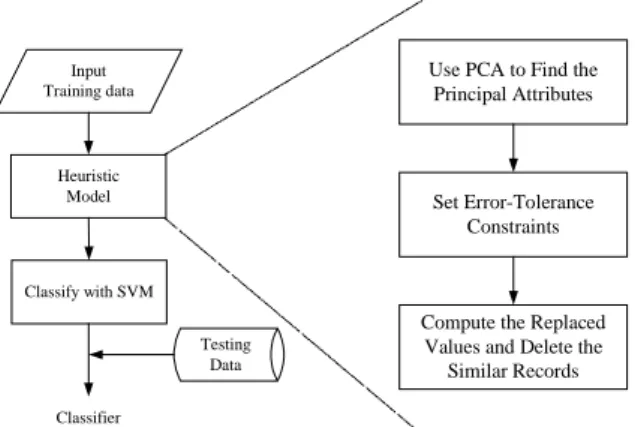
(3) Int. Computer Symposium, Dec. 15-17, 2004, Taipei, Taiwan.. ∑α. s.t.. i yi∈Class1. (αi. ∑α. =1. i yi∈Class −1. =1. Heuristic Model. Then, we want to maximize the margin between two parallel supporting planes. A plane supports a class if all points in that class if all points in that class are no one side of that plane. For the points with the class label +1 we would like there to exist w and b such that w. xi > b or w. xi – b > 0 depending on the class label. We can simply maximize the distance or margin between the support planes for each class. The distance or margin between these supporting planes w. x = b and w. x = b – 1 is. γ. = 2/. Testing Data. w,b. s.t. The. Figure 3.1 The framework of the Heuristic Model. 3.1 Finding the Principal Attributes by PCA. w 2 /2 in the following. In data mining, there will be usually large number of variables in the database. The accuracy and reliability of a classification or prediction model will suffer if you include highly correlated variables or variables that are unrelated to the outcome. Superfluous variables increase the data-collection and data-processing costs to deploy a model on a large database. The dimensionality of a model is the number of independent or input variables used by the model. One of the key steps in data mining is finding ways to reduce dimensionality without sacrificing accuracy. Principal component analysis (PCA) is a mathematical procedure that transforms a number of (possibly) correlated variables into a (smaller) number of uncorrelated variables called principal components. The main use of PCA is to reduce the dimensionality of a data set while retaining as much information as is possible. It computes a compact and optimal description of the data set. The first principal component is the combination of variables that explains the greatest amount of variation. The second principal component defines the next largest amount of variation and is independent to the first principal component. There can be as many possible principal components as there are variables. In this research, we use Weka to find the principal attributes and it will be described later.. y i (w ⋅ x i. 1 2 w 2 w. xi ≥ b + 1. yi ∈ Class 1 W . xi ≤ b + 1 yi ∈ Class -1. constraints − b) ≥ 1 .. can. be. simplified. Compute the Replaced Values and Delete the Similar Records. Classifier. quadratic program:. min. Set Error-Tolerance Constraints. Classify with SVM. w 2 . Thus maximizing the margin. is equivalent to minimize. Use PCA to Find the Principal Attributes. Input Training data. ≥ 0 , i = 1,….,m). to. 2.5 Summary The SVMs have been introduced for almost 10 years. There are many studies focus on its concepts and principle [3], [7]. Some studies research the applications of its [8]. And some studies explore the ability of multi-category for SVM [6]. The SVMs are not always the best, it still requires skill to apply them and other methods may be better suited for particular applications. There are more and more studies confer the kernels [1]. It is not easy to develop a good kernel, and it is hard to find the suitable kernel (including its parameters) for different cases. There are fewer studies considering the data preprocessing of SVMs. In the study, we hope to find a way that can effectively and efficiently reduce the input space for the characteristics of SVMs.. 3.2 Error-Tolerance Constraints After finding out the principal attributes, we can set the error-tolerance constraints if needed. In general, if the principal attributes all belong to discrete types, and the categories are not many, we don’t need to set the error-tolerance constraints. But if some principal attributes belong to continuous types or the categories are many, we have to set the error-tolerance constraints. Who will set the error-tolerance constraints? That is the man who has the specialized knowledge for the domain of the database. For this research, there will be five different datasets from UCI database. The. 3. Methodology The theme of the methodology includes three parts. Figure 3.1 is the framework of the Heuristic Model.. 376.

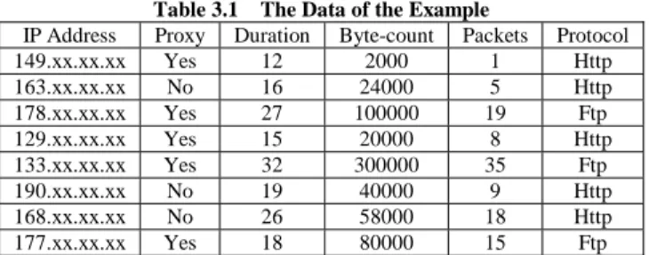
(4) Int. Computer Symposium, Dec. 15-17, 2004, Taipei, Taiwan. found principal attributes of three of them need not to set the error-tolerance constraints, because the principal attributes all belong to discrete types and the categories are not many. The other two datasets are medical; therefore we have been to hospitals to consult the doctor. Then set the error-tolerance constraints according to the suggestion of the doctor.. 3.3 Replaced Values Computation Similar Records Deletion. 3.4.1 Finding the Principal Attributes by PCA for Example There are a lot of software for the data mining, such as ID3, C4.5, S plus, and Weka. They almost can help us to find the principal attributes of databases but for the consistency of software, we select the Weka, which can support the packages of SVM. Weka reads database in ARFF format. It is necessary to have type information of each attribute because that can’t be automatically deduced form the attribute values. So we must convert our data to ARFF form. The ARFF file consists of a list of all the instances with the attribute values being separated by commas. The most important thing is we have to add the dataset’s name using the @relation tag, the attribute information using @attribute, and a @data; then save the file as filename.ARFF. After converting our data to ARFF form with necessary tags, we can use the package of Principle Components in Weka Explorer to find the principle attributes.. and. After setting the error-tolerance constraints, we can compute the replaced value for found principal attributes. Then, we search and delete the similar records which have the same replaced values of selected principal attributes. The algorithm as following: Step1. Select the next principal attribute, if none, go to Step 4. Step2. For the selected principal attribute (step1), sort the records by values of the attribute increasingly. Step3. Compute the replaced values. Step 3.1 Select the next value, if none, go to Step1. Step 3.2 Add (2 * error-tolerance) to the current value. Step 3.3 Select the next value. Step 3.4 If the value (Step3.3) < the sum (Step3.2) /* within the error-tolerance Use the sum replaced the value (3.3), and go to Step 3.4 Else go to Step 3.1. Step4. Search the similar records which have the same replaced values of selected principal attributes. Step5. Select the ordinal of (n+1)/2 record from the similar records and delete the other redundant similar records. Step6. Restore the values of all selected records.. 3.4.2 Error-Tolerance Example. 3.4.3 Replaced Values Computation and Similar Records Deletion for Example After setting the error-tolerance constraints, we can compute the replaced value for found principal attributes – byte-count and packet. After the program processing, the replaced values are shown at Table 3.2.. Now we use a simple example to illustrate how we process with the proposed heuristic model. The data of the example is shown as Table 3.1. The class attribute is Internet Protocol. Table 3.1 The Data of the Example Proxy Duration Byte-count Packets Yes 12 2000 1 No 16 24000 5 Yes 27 100000 19 Yes 15 20000 8 Yes 32 300000 35 No 19 40000 9 No 26 58000 18 Yes 18 80000 15. for. The found principle attributes for our example are Byte-count and Packages that belong to the continuous type of data. Therefore we have to set the error-tolerance constraints. We assume the error-tolerance of byte-count is 25000, and the error-tolerance of packet is 4.. 3.4 A Simple Example. IP Address 149.xx.xx.xx 163.xx.xx.xx 178.xx.xx.xx 129.xx.xx.xx 133.xx.xx.xx 190.xx.xx.xx 168.xx.xx.xx 177.xx.xx.xx. Constraints. Protocol Http Http Ftp Http Ftp Http Http Ftp. 377. Table 3.2 Computed Replaced Values Byte-count Packets Protocol 2000 Æ 52000 1Æ9 Http 24000 Æ 52000 5Æ9 Http 100000 Æ 108000 19 Æ 19 Ftp 20000 Æ 52000 8Æ9 Http 300000 Æ 350000 35 Æ 44 Ftp 40000 Æ 52000 9Æ9 Http 58000 Æ 108000 18 Æ 19 Http 80000 Æ 108000 15 Æ 19 Ftp Then, we search the similar records with the same replaced values of selected principal attributes. For easily to illustrate, we sort and re-categorize the records as shown at Table 3.3..

(5) Int. Computer Symposium, Dec. 15-17, 2004, Taipei, Taiwan.. Table 3.3 Re-Categorized Result Byte-count Packets Re-categorize 2000 Æ 52000 1Æ9 A 20000 Æ 52000 8Æ9 A 24000 Æ 52000 5Æ9 A 40000 Æ 52000 9Æ9 A 58000 Æ 108000 18 Æ 19 B 80000 Æ 108000 15 Æ 19 B 100000 Æ 108000 19 Æ 19 B 300000 Æ 350000 35 Æ 44 C. Table 4.2 Summary of Results of Second Experiment Precision (%). Table 3.5 Final Data Duration Byte-count 16 24000 32 300000 18 80000. 82.8241. 92.3077. 55.9846. 83.2326. 71.0526. 66.2791. 81.7435. Training. 96.7181. 77.9923. 88.8889. 55.8774. 77.3234. Bayes. Testing. 98.8439. 81.9767. 71.0526. 43.0233. 76.9565. RBF. Training. 94.6768. 52.8958. 84.6154. 59.4595. 65.6134. Network. Testing. 95.9538. 63.9535. 65.7895. 62.7907. 66.5217. Naïve. Table 4.3 Summary of Results of Third Experiment. Original Input space. Improved Input space. Protocol Http Ftp Ftp. Training Instances Time (sec.) Testing Precision Training Instances Time (sec.) Testing Precision. Breast Cancer. Credit Screening. Hepatitis. Liver Disorder. Pima. 526. 518. 117. 259. 576. 0.62. 1.7. 0.48. 1.02. 0.52. 98.69. 83.23. 71.05. 66.28. 81.74. 143. 173. 67. 121. 165. 0.23. 0.38. 0.2. 0.41. 0.24. 97.69. 82.99. 74.49. 65.87. 82.18. 5. Conclusions and Future Works By using the SVM with Weka to make a classifier, we can use the classifier to predict the given testing data. In this research, we propose the heuristic model and test it by using real database from UCI database practically. We do some experiments in previous section, and verify that the performance of SVM is well and the heuristic model can achieve the objective.. 4. Experimental Results We use full-training-set in Weka and the results manifest that the precision of SVM are actually better than Naïve Bayes and RBF Network by using the five different datasets (see Table 4.1). Table 4.1 Summary of Results of First Experiment Precision Breast Credit Liver Hepatitis (%) Cancer Screening Disorder SVM 98.9986 85.942 88.3871 58.2609 Naïve Bayes 97.4274 78.2609 85.8065 56.8116 RBFNetwork 95.7082 64.2029 80.6452 58.1304. 77.7658. Then, the most important is that we focus on the performance of the heuristic method, which was proposed in the research, and the Table 4.3 is the summary of results of experiment. We can see the heuristic method actually reduced the instances and execution time. And we still find the precision of the heuristic method is better than expected. In the beginning, we just want to make the precision can be in an acceptable range, but the results shown that the objective is actually can be achieved. Otherwise, it maybe makes the precision to be enhanced (With the Hepatitis and Pima Indians Diabetes Datasets).. Re-categorize A B C. Packets 5 35 15. Pima. 98.0134. At last, we restore the values of all selected records (see Table 3.5) and we will put the data to train the classifier of SVM by Weka. We will do some experiments by Weka with the UCI Database and compare with three different classification methods (RBFNetwork, Naïve Bayes, and SVM) in next section. Proxy No Yes Yes. Liver Disorder. 98.6879. Precision (%). IP Address 163.xx.xx.xx 133.xx.xx.xx 177.xx.xx.xx. Hepatitis. Testing. Table 3.4 Result of Deleted the Similar Records. Packets 5Æ9 15 Æ 19 35 Æ 44. Credit Screening. Training. SVM. According to the Table 3.3, we select the ordinal of (n+1)/2 records from the similar records and delete the other redundant similar records. The result was shown as Table 3.4. By the example, we successfully reduce the records within the set error-tolerance. Byte-count 24000 Æ 52000 80000 Æ 108000 300000 Æ 350000. Breast Cancer. Pima. 5.1 Conclusions. 77.474 76.3021 65.8854. Through the experimental results, we can see the performance of SVM is better than Naïve Bayse and NBF Network by using full-training-set for the five different datasets. The performance of SVM is still the best by using training-testing-set. No matter for the training or testing, SVM has the better precision for any datasets. For generalization, SVM seems to be good than NBF Network, but is not distinctly better than Naïve Bayse. And we find that the chosen datasets will affect the experimental results seriously. Like for the Breast Cancer Datasets, the SVM, Naïve Bayse and. In Table 4.2, we can see the precision of SVM are better than Naïve Bayes and RBFNetwork by using the five different datasets (see Table 4.2). For training, SVM is the best; for testing, SVM is only little loser than Naïve Bayes on Breast Cancer Dataset. Through the Table 4.2, we also find the generalization of SVM is better. Since the precision of SVM is not all the best for testing, but the range of rise (Training -> Testing) is better.. 378.

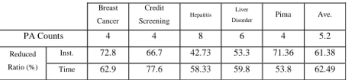
(6) Int. Computer Symposium, Dec. 15-17, 2004, Taipei, Taiwan. kernel. Therefore, we can find better software or wait Weka to update that can support more kernels to do experiments. After all, the Weka is actually easy to use and powerful. In addition to test it for more kernels, we still can test for the classification of multi-class.. NBF Network all have the greatest precision no matter for the training or testing; and for the Liver Disorder Datasets, they all have the worst precision during the training and testing. The performance of the heuristic method, which was proposed in this research, we can see the heuristic method actually reduced the instances and execution time. For the instances, the average of reduced ratio is about 61.38%, and the average of reduced ratio is about 62.4% for the execution time. The reduced ratio is correlated with the principal attributes of datasets that found by Weka (see Table 5.1). We found that the principal attributes of Breast Cancer, Credit Screening, and Pima Indians Diabetes Datasets are all four items, and therefore the reduced ratio of instances can be obvious.. References [1]. [2]. Table 5.1 Summary of the Reduced Ration for Instances and Execution Time Breast. Credit. Cancer. Screening. 4. 4. 8. Liver. Hepatitis. PA Counts. Pima. Ave.. 6. 4. 5.2. Disorder. Reduced. Inst.. 72.8. 66.7. 42.73. 53.3. 71.36. 61.38. Ratio (%). Time. 62.9. 77.6. 58.33. 59.8. 53.8. 62.49. [3]. [4] And we found that after our heuristic model processing, the reduced ratio for the precision is satisfied with us. For Breast Cancer, Credit Screening and Liver Disorder Datasets, the precisions are all worst than before, but the ratio is not more than 1% (see Table 5.2). Even for Hepatitis and Pima Indians Diabetes Datasets, the precisions are both better than before. It is beyond our expectations.. [5]. [6]. Table 5.2 Summary of the Reduced Ratio for Precision Breast. Credit. Cancer. Screening. -0.73. -0.29. Liver Hepatitis. Reduced Ratio (%). Disorder 4.8. -0.62. [7]. Pima. 0.53. [8]. We think the reason might be the original input space with a little impure data. In the training phase of SVM, SVM will automatically use a tradeoff parameter with penalty functions to deal with the noises. If the noises are too many, it might affect the produce of classifier with SVM. But after processing of our heuristic model, it could be reduced the impure data and resulted in the raise of precision.. [9]. 5.2 Future Works The compression technique in the phase of replaced values computation is based on heuristic relation. We’ll refer to some robust methods to improve the performance, such as: vector quantization, entropy, and other data compression technology. We believe the experience in the area of data compression can give help in our research. In practice, there are many kernels applied in various areas. Weka just provides the polynomial. 379. N.E. Ayat, M. Cheriet, L. Remaki, and C.Y. Suen, “KMOD- a New Support Vector Machine Kernel With Moderate Decreasing for Pattern Recognition. Application to Digit Image Recognition”, pp.1215-1219, 2001. C. Burges, “A tutorial on support vector machines for pattern recognition”, Data Mining and Knowledge Discovery, pp.121-167. , 1998, K.P. Bennett, and C. Campbell, “Support vector machines: Hype or hallelujah?” ACM SIGKDD Explorations Newsletter, pp.1-13, 2000. K.P. Bennett, D. Hui, and L Auslender, “On support vector decision trees for database marketing”, Department of Mathematical Sciences Math Report, pp98-100, 1998. M. P. S. Brown, W. N. Grundy, D. Lin, and Haussler, D. etc., “Knowledge-based analysis of microarray gene expression data using support vector machines”, pp.262-267, 2000. S. Babu, M. Garofalakis, and R. Rastogi, “SPARTAN:Using Constrained Models for Guaranteed-Error Semantic Compression”, ACM SIGKDD Explorations Newsletter, 2002. F. Cortes, and V. Vapnik, “Support Vector Networks”, Machine Learning, vol.20, pp.273-297, 1995. N. Cristianini, and J. S. Taylor, “An Introduction to Support Vector Machines and other Kernel-based Learning Methods”, Cambridge University Press, 2000. H. Hermes, and J. M. Buhmann, “Feature Selection for Support Vector Machines”, Proc. of the IEEE, pp.712-715, 2000..

(7)