NEURO-FUZZY MODELING AND CONTROL

(1)

Neuro-Fuzzy Modeling

and

Control

JYH-SHING ROGER JANG,

MEMBER, IEEE, AND

CHUEN-TSAI SUN,

MEMBER, IEEE

Fundamental and advanced developments in neum-fuzzy syner- gisms f o r modeling and control are reviewed. The essential part of neuro-fuuy synergisms comes from a common framework called adaptive networks, which unifies both neural networks and fuzzy models. The f u u y models under the framework of adaptive net- works is called Adaptive-Network-based Fuzzy Inference System (ANFIS), which possess certain advantages over neural networks. We introduce the design methods f o r ANFIS in both modeling and control applications. Current problems and future directions f o r neuro-fuzzy approaches are also addressed.

modeling. neuro-fuzzy control. ANFIS.

Keywords- F u u y logic, neural networks, fuzzy modeling, neuro-fuzzy

I. INTRODUCTION

In 1965, Zadeh published the first paper on a novel way of characterizing nonprobabilistic uncertainties, which he called “fuzzy sets” [116]. This year marks the 30th anniversary of fuzzy logic and fuzzy set theory, which has now evolved into a fruitful area containing various disciplines, such as calculus of fuzzy if-then rules, fuzzy graphs, fuzzy interpolation, fuzzy topology, fuzzy reasoning, fuzzy inferences systems, and fuzzy modeling. The applications, which are multi-disciplinary in nature, includes automatic control, consumer electronics, signal processing, time-series prediction, information retrieval, database management, computer vision, data classification, decision-making, and so on.

Recently, the resurgence of interest in the field of artificial neural networks has injected a new driving force into the “fuzzy” literature. The back-propagation learning rule, which drew little attention till its applications to artificial neural networks was discovered, is actually an universal learning paradigm for any smooth parameterized models, including fuzzy inference systems (or fuzzy models). As

a result, a fuzzy inference system can now not only take linguistic information (linguistic rules) from human experts, but also adapt itself using numerical data (input/output pairs) to achieve better performance. This gives fuzzy Manuscript received March 30, 1994; revised November 28, 1994. This work was supported in part by NASA Grant NCC 2-275, MICRO Grant 92-180, EPRl Agreement RP 8010-34, and in part by the BISC program. J . 4 . Jang is with the Control and Simulation Group, The Mathworks, Inc., Natick, MA 01760 USA.

C.-T. Sun is with the Department of Computer and Information Science,

National Chiao Tung University, Hsinchu, Taiwan. IEEE Log Number 940830 1 .

inference systems an edge over neural networks, which cannot take linguistic information directly.

In this paper, we formalize the adaptive networks as a universal representation for any parameterized models. Under this common framework, we reexamine back- propagation algorithm and propose speedup schemes utilizing the least-squared method. We explain why neural networks and fuzzy inference systems are all special instances of adaptive networks when proper node functions are assigned, and all leaming schemes applicable to adaptive networks are also qualified methods for neural networks and fuzzy inference systems.

When represented as an adaptive network, a fuzzy inference system is called adaptive networks-based fuzzy inference systems (ANFIS). For three of the most commonly used fuzzy inference systems, the equivalent ANFIS

can be derived directly. Moreover, the training of ANFIS

follows the spirit of the m i n i m u m disturbance p r i n c i p l e [lo91 and is thus more efficient than sigmoidal neural networks.

Once a fuzzy inference system is equipped with learning capability, all the design methodologies for neural network controllers become directly applicable to fuzzy controllers. We briefly review these design techniques and give related references for further studies.

The arrangement of this article is as follows. In Section 11, an in-depth introduction to the basic concepts of fuzzy sets, fuzzy reasoning, fuzzy if-then rules, and fuzzy inference systems are given. Section 111 is devoted to the formaliza- tion of adaptive networks and their leaming rules, where the back-propagation neural network and radial basis function network are included as special cases. Section IV explains

the ANFIS architecture and demonstrates its wperiority over back-propagation neural networks. A number of design techniques for fuzzy and neural controllers is described in Section V . Section VI concludes this paper by pointing out current problems and future directions.

11.

REASONING, AND FUZZY MODELS

FUZZY SETS, FUZZY RULES, F U 7 . y

This section provides a concise introduction to and a summary of the basic concepts central to the study of fuzzy sets. Detailed treatments of specific subjects can be found in the reference list.

378

0018-9219/95$04.00 0 1995 IEEE

(2)

MF on a diwntc X

I ’ I MF an a continuous x

X = numbcr of courses X = age

Fig. 1.

“about 50 years (a) A = old.” “appropriate number of courses taken” (b) B =

A. Fuzzy Sets

example, a classical set A can be expressed as

A classical set is a set with a crisp boundary. For

A = {z

I

z

>

6) (1) where there is a clear, unambiguous boundary point 6 such that if z is greater than this number, then z belongs to the set A, otherwise z does not belong to this set. In contrast to a classical set, a fuzzy set, as the name implies, is a set without a crisp boundary. That is, the transition from “belonging to a set” to “not belonging to a set” is gradual, and this smooth transition is characterized by membership functions that give fuzzy sets flexibility in modeling commonly used linguistic expressions, such as “the water is hot” or “the temperature is high.” As Zadeh pointed out in 1965 in his seminal paper entitled “Fuzzy Sets” [ 1 161, such imprecisely defined sets or classes “play an important role in human thinking, particularly in the domains of pattem recognition, communication of information, and abstraction.” Note that the fuzziness does not come from the randomness of the constituent members of the sets, but from the uncertain and imprecise nature of abstract thoughts and concepts.

Dejnition 1: Fuzzy Sets and Membership Functions If X is a collection of objects denoted generically by z, then a fuzzy set A in X is defined as a set of ordered pairs:

p ~ ( z ) is called the membership function (MF for short) of 2 in A. The MF maps each element of X to a continuous membership value (or membership grade) between 0 and 1.

0

Obviously the definition of a fuzzy set is a simple extension of the definition of a classical set in which the characteristic function is permitted to have continuous values between 0 and 1. If the value of the membership function p . ~ ( z ) is restricted to either 0 or 1, then tl is reduced to a classical set and p . A ( r ) is the characteristic function of A .

Usually X is referred to as the “universe of discourse,” or simply the “universe,” and it may contain either discrete objects or continuous values. Two examples are given below.

Example 1: Fuuy Sets with Discrete X . Let X = { 1, 2, 3, 4, 5 . 6, 7, 81 be the set of numbers of courses a student

may take in a semester. Then the fuzzy set A = “appropriate number of courses taken” may be described as follows:

A ={(11~.1),(2,0.~~,(~l~~.~)l(~, I ) , (5,0.9),(6,0.5),(7,0.2),(8,0.1)}. This fuzzy set is shown in Fig. ](a).

0

Example 2: Fuzzy Sets with Continuous X . Let X = R+

be the set of possible ages for human beings. Then the fuzzy set B = “about 50 years old” may be expressed as

B = {(z.,u”B(.r) 15 E

X}

where

This is illustrated in Fig. l(b). U

An alternative way of denoting a fuzzy set A is p ~ ( z , ) / ~ , , if X is discrete.

(3) A = X T € ? X -

S,

p ~ A ( : r ) / r l if

x

is continuous.

{

The summation and integration signs m (3) stand for the union of (2. p~ ( . E ) ) pairs; they do not indicate summation or integration. Similarly,

“/”

is only a marker and does not imply division. Using this notation, we can rewrite the fuzzy sets in Examples 1 and 2 as

A = O . l / l

+

0.3/2

+

0.8/3

+

1.0/1

+

0.9/5

+

0.5/6

+

0.2/7

+

0.1/8, and

respectively.

From Example 1 and 2, we see that the construction of a fuzzy set depends on two things: the identification of a suitable universe of discourse and the specification of an appropriate membership function. It should be noted that the specification of membership functions is quite subjective, which means the membership functions specified for the same concept (say, “cold”) by different persons may vary considerably. This subjectivity comes from the indefinite nature of abstract concepts and has nothing to do with randomness. Therefore the subjectivity and nonrandomness of fuzzy sets is the primary difference between the study of fuzzy sets and probability theory, which deals with objective treatment of random phenomena.

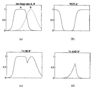
Corresponding to the ordinary set operations of union, intersection, and complement, fuzzy sets have similar operations, which were initially defined in Zadeh’s paper [116]. Before introducing these three fuzzy set operations, first we will define the notion of containment, which plays a central role in both ordinary and fuzzy sets. This definition of containment is, of course, a natural extension of the case for ordinary sets.

(3)

two fuzzy gets A, B

" A OR B"

"NOT A

I'

"A AND E"

I

't

Fig.?.

(b) 4 ; ( c ) A U 8 ; (d) -4 f l B .

Operations on fuzzy sets: (a) two fuzzy sets A and B ;

Definition 2: Containment or Subset Fuzzy set A is con-

tained in fuzzy set B (or, equivalently, A is a subset of

B ,

or

A is smaller than or equal to B ) if and only if

PA(%)

5

p ~ ( x ) for all z. In symbols,

(4)

0

Definition 3: Union (disjunction) The union of two fuzzy sets A and B is a fuzzy set C , written as C = A U B

or C = A OR

B,

whose MF is related to those of A

and B by

A

c

B

e

P A ( x )

5

P B ( x ) .

p C ( X ) = " ( b A ( Z ) , b B ( x ) ) = P A ( z ) V P B ( x ) . ( 5 ) U As pointed out by Zadeh [116], a more intuitive and appealing definition of union is the smallest fuzzy set containing both

A

and B. Alternatively, if D is any fuzzy set that contains both A and B, then it also contains A U B.

The intersection of fuzzy sets can be defined analogously.

Definition 4: Intersection (conjunction) The intersection of two fuzzy sets A and B is a fuzzy set C , written as

C = A fl B or C = A AND B, whose MF is related to those of A and B by

P C ( z ) = min(pA(x), p L ? ( z ) ) = pA(z) A P B ( x ) . ( 6 )

0

As in the case of the union, it is obvious that the intersection of A and B is the largest fuzzy set which is contained in both A and B. This reduces to the ordinary intersection operation if both A and B are nonfuzzy.

Definition 5: Complement (negation) The complement of fuzzy set A , denoted by ~ ( T A , NOT A ) , is defined as

p x ( x ) = 1 - P A ( Z ) . (7)

0

Fig. 2 demonstrates these three basic operations: 1) illustrates two fuzzy sets A and B , 2) is the complement of

A , 3) is the union of A and B , and 4) is the intersection

of

A

and

B.

Note that other consistent definitions for fuzzy AND and OR have been proposed in the literature under the names "T-norm" and "T-conorm" operators [ 161, respectively. Except for min and max, none of these operators satisfy the law of distributivity:

pAU(BnC)(2) = /L(AUB)n(AUC)(X), PAn(BUC)(l) = P(AI~B)V(A"C)(~). However, min and max do incur some difficulties in ana- lyzing fuzzy inference systems. A popular alternative is to use the probabilistic AND and OR:

pAnB(z) = /LA(x)PB(z).

p A u B ( z ) = p A ( z ) -k P B ( T ) - P A ( x ) P B ( z ) . In the following, we shall give several classes of parameterized functions commonly used to define MF's. These parameterized MF's play an important role in adaptive fuzzy inference systems.

Definition 6: Triangular MF's A triangular M F is spec- ified by three parameters { a , b. c}, which determine the z coordinates of three comers:

triangle(:c; a , b, c )

= rnax (min

(-,-),o).

2 - a c - x ₍₈₎ h - U C - b

Fig. 3(a) illustrates an example of the triangular MF defined

0

Definition 7: Trapezoidal M F ' s A trapezoidal M F is

by triangle(x; 20, 60, 80).

specified by four parameters { U , b. c. d } as follows:

trapezoid(.c: a , b, c . d )

= max (rriin

(E,

x - a 1 ,

----)

d - 3 . ,(I). (9)

d - ( .

Fig. 3(b) illustrates an example of a trapezoidal MF defined by trapezoid(x; 10, 20, 60, 95). Obviously, the triangular

0

Due to their simple formulas and computational effi- ciency, both triangular MF's and trapezoidal MF's have been used extensively, especially in real-time implementa- tions. However, since the MF'\ are composed of straight line segments, they are not smooth at the switching points specified by the parameters. In the following we introduce other types of MF's defined by smooth and nonlinear functions.

Definition 8: Gaussian M F ' s A Gaussian M F is specified by two parameters {g. c}:

MF is a special case of the trapezoidal MF.

gaussian(2; f7* c ) = , { - [ ( x - c ) / ~ I L } ₍₁₀₎

where c represents the MF's center and c determines the MF's width. Fig. 3(c) plots a Gaussian MF defined by

gaussian(x;20,50).

0

(4)

hianguler MF

X

(a)

Gaussian MF bell MF

X

Fig. 3. Examples of various classes of MF’s: (a) t r r a n g l e (x; 20, 60, 80); (b) t r a p e z o i d ( x ; IO, 20, 60, 95); ( c ) gaussic~n (x; 20, 50); (d) bell (x; 20, 4, 50).

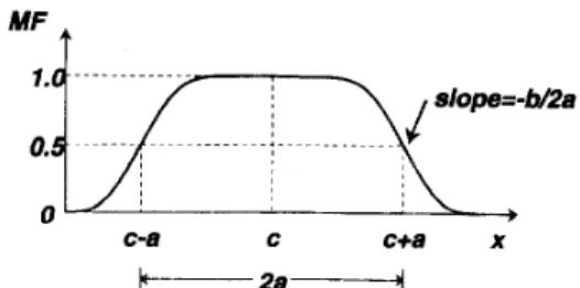
Deifinition 9: Generalized Bell MF’s A generalized bell

MF (or bell MF ) is specified by three parameters {a, b , c}:

where the parameter b is usually positive. Note that this MF

is a direct generalization of the Cauchy distribution used in probability theory. Fig. 3 illustrates a generalized bell MF U A desired generalized bell MF can be obtained by a proper selection of the parameter set { a . b. c } . Specifically, we can adjust c and a to vary the center and width of the MF, and then use b to control the slopes at the

crossover points. Fig. 4 shows the physical meanings of each parameter in a bell MF.

Deifinition IO: Sigmoidal M F ’ s A sigmoidal MF is defined by defined by bel@; 20, 4, 50). (12) 1 1

+

exp [-a(. - c)] s i g m o i d ( x ; a . c) =

where a controls the slope at the crossover point x = c. 0

Depending on the sign of the parameter a , a sigmoidal

MF is inherently open right or left and thus is appropriate for representing concepts such as “very large” or “very negative.” Sigmoidal functions of this kind are employed widely as the activation function of artificial neural networks. Therefore, for a neural network to simulate the behavior of a fuzzy inference system, the first problem we face is how to synthesize a close MF through a sigmoidal function. There are two simple ways to achieve this: one is

Fig. 4. Physical meaning of parameters in a generalized bell function.

to take the product of two sigmoidal MF’s; the other is to take the absolute difference of two sigmoidal MF’s.

It should be noted that the list of MF’s introduced in this section is by no means exhaustive; other specialized MF’s can be created for specific applications if necessary. In particular, any types of continuous probability distribution functions can be used as an MF here, provided that a set of parameters are given to specify the appropriate meanings of the MF.

B. Fuzzy If-Then Rules

conditional statement ) assumes the form

A fuzzy if-then rule (fuzzy rule, fuzzy implication, or fuzzy

if x is A then y is B (13) where A and B are linguistic values defined by fuzzy sets on universes of discourse X and Y , respectively. Often

“x is A” is called the antecedent or premise while “y is

B” is called the consequence or conclusion. Examples of fuzzy if-then rules are widespread in our daily linguistic expressions, such as the following:

If pressure is high then volume is small. If the road is slippery then driving is dangerous. If a tomato is red then it is ripe.

If the speed is high then apply the brake a little. Before we can employ fuzzy if-then rules to model and analyze a system, we first have to formalize what is meant by the expression “if x is A then y is B,” which is sometimes abbreviated as

.4

+ R. In essence, the expression describes a relation between two variables x and y; this suggests that a fuzzy if-then rule be defined as a

binary

fuzzy

relation R on the product space X

x

Y . Note that a binary fuzzy relation R is an extension of the classical Cartesian product, where each element (x,y) E X

x

Y is associated with a membership grade denoted by p ~ ( x , y). Altematively, a binary fuzzy relation R can be viewed as a fuzzy set with universe X x Y , and this fuzzy set is characterized by a two-dimensional MF p~ ( x . y ).

Generally speaking, there are two ways to interpret the fuzzy rule A -+ B. If we interpret A --+ B as ‘ * A coupled with B,” then

R = A + B = A x B =

(5)

B

T x

Y

x

(a) (b)

Two interpretations of fuzzy implication: (a) A coupled Fig. 5.

with B ; (b) A entails E .

where i is a fuzzy AND (or more generally, T-norm) operator and A -+

B

is used again to represent the fuzzy relation R. On the other hand, if A -+ B is interpreted as “ A entails B,” then it can be written as four different formulas:

Material implication: R = A -+ B = T A U B .

Propositional calculus: R = A + B = - A U ( A

n

B ) .

Extended propositional calculus: R = A -+ B = (’A

n

’ B ) U B.

Generalization of modus ponens: p ~ ( x , y ) =

~ u p { c ( p ~ ( x ) * c

5

p ~ ( y ) a n d O

5

c

I

l}, where

R = A -+ B and jl is a T-norm operator.

Though these four formulas are different in appearance, they all reduce to the familiar identity A -+ B T A U B

when A and B are propositions in the sense of two-valued logic. Fig. 5 illustrates these two interpretations of a fuzzy rule A -+ B . Here we shall adopt the first interpretation,

where A -+ B implies “ A coupled with B.” The treatment of the second interpretation can be found in [35], [50], [Sl].

C. Fuzzy Reasoning (Approximate Reasoning)

Fuzzy reasoning (also known as approximate reasoning)

is an inference procedure used to derive conclusions from a set of fuzzy if-then rules and one or more conditions. Before introducing fuzzy reasoning, we shall discuss the compositional rule of inference [ 1171, which is the essential rationale behind fuzzy reasoning.

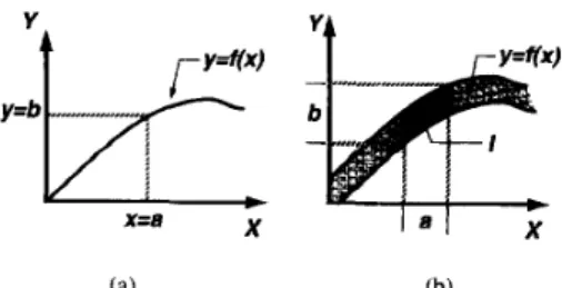
The compositional rule of inference is a generalization of the following familiar notion. Suppose that we have a curve y =

f(z)

that regulates the relation between x and y. When we are given z = a , then from y = f ( x ) we can infer that y = b = f(a); see Fig. 6(a). A generalization of the above process would allow a to be an interval and f(z) to be an interval-valued function, as shown in Fig. 6(b). To find the resulting interval y = b corresponding to the interval x = a, we first construct a cylindrical extension of a (that

is, extend the domain of a from X to X x Y ) and then find its intersection I with the interval-valued curve. The projection of I onto the y-axis yields the interval y = b.

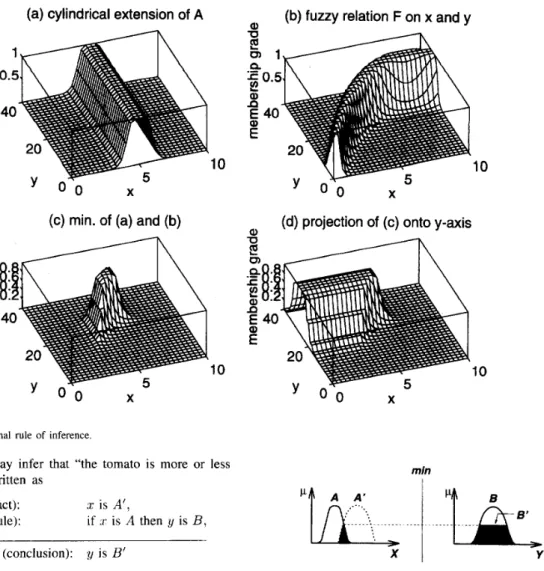
Going one step further in our generalization, we assume that A is a fuzzy set of X and F is a fuzzy relation on

X x

Y ,

as shown in Fig. 7(a) and (b). To find the resulting

fuzzy set B , again, we construct a cylindrical extension

c ( A ) with base A (that is, we expand the domain of A from

X to

X

x Y to get c ( A ) ) . The intersection of c ( A ) and F

(Fig. 7(c)) forms the analog of the region of intersection I

(a) (b)

Fig. 6. Derivation of y = b from .c = a and y = f(.c). (a) a and b are points, y = f ( z ) is a curve, (b) a and b are intervals, y = f(s) IS an interval-valued function.

in Fig. 6(b). By projecting c ( A )

n

F onto the y-axis, we infer y as a fuzzy set B on the y-axis, as shown in Fig. 7(d). Specifically, let P A , p c ( ~ ) , p ~ , and p~ be the MF’s of A , c ( A ) , B, and F , respectively, where p , ( ~ ) is related to p~ through

Y) = p A ( X ) . Then

This formula is referred to as m a - m i n composition and B

is represented as

B = A o F

where o denotes the composition operator. If we choose product for fuzzy AND and max for fuzzy OR, then we have ma-product composition and p g ( y ) is equal Using the compositional rule of inference, we can formalize an inference procedure, called fuzzy reasoning, upon a set of fuzzy if-then rules. The basic rule of inference in traditional two-valued logic is modus ponens, according to which we can infer the truth of a proposition B from the truth of A and the implication A + B . For instance, if

A is identified with “the tomato is red” and B with “the tomato is ripe,” then if it is true that “the tomato is red,” it is also true that “the tomato is ripe.” This concept is illustrated below. vx [ p A ( Z : ) p F ( x , U)]. premise 1 (fact): premise 2 (rule): x is A , if z is A then :y is B , ~ consequence (conclusion): y is B.

However, in much of human reasoning, modus ponens is employed in an approximate manner. For example, if we have the same implication rule “if the tomato is red then it is ripe” and we know that “the tomato is more or less

(6)

(a) cylindrical extension of A

(b)

fuzzy relation

F

on x and y

Q,

10

10 (c) min. of (a) and (b)

(d) projection of (c) onto y-axis

a

Q,

U

10 10

ripe.” This is written as

premise 1 (fact): x is A’,

YT/jl:

...,,,,, >

premise 2 (rule):

consequence (conclusion): ?/ is B‘ X

if :I‘ is A then y is B,

...-...

....

Fig. 7. Compositional rule of inference

I&,>

~ ... . ....

Y where A‘ is close to A and B’ is close to

B.

When A ,

B, A’, and

B’

are fuzzy sets of appropriate universes, the above inference procedure is called fuzzy reasoning or approximate reasoning; it is also called generalized m o d u s ponens, since it has modus ponens a5 a special case.

Using the composition rule of inference introduced earlier, we can formulate the inference procedure of fuzzy reasoning as the following definition.

Dejiinitian 1 I: Fuzzy Reasoning Bused On M a - M i n Com- position: Let A , A‘, and B be fuzzy sets of X , X , and Y ,

respectively. Assume that the fuzzy implication A + B is expressed as a fuzzy relation R on X x Y . Then the fuzzy set B’ induced by “lc is A’” and the fuzzy rule “if x is A then y is B” is defined by

Fig. 8. Fuzzy reasoning for a single rule with a single antecedent.

Remember that (15) is a general expression for fuzzy reasoning, while (14) is an instance of fuzzy reasoning where min and max are the operators for fuzzy AND and OR, respectively.

Now we can use the inference procedure of the generalized modus ponens to derive conclusions, provided that the fuzzy implication A --+ B is defined as an appropriate

binary fuzzy relation.

1) Single Rule with Single Antecedent For a single rule with a single antecedent, the formula is available in (14). A further simplification of the equation yields

p ~ , ( y ) = max min [ p A , ( s ) , p R ( x , y ) ] P B ’ ( z l ) = [ v x (P.4,(Z) A PA-L(2)] A P B ( Y )

X

= ? U A p ~ ( y ) .

=

v.r

[ P A ’ ( Z ) A p R ( . c , y)] (14)

In other words, first we find the degree of match w as the maximum of ~ A , ( z ) A p , 4 ( z ) (the shaded area in the antecedent part of Fig. 8); then the MF of the resulting B’

is equal to the MF of B clipped by 20, shown a? the shaded area in the consequent part of Fig. 8.

or, equivalently,

R‘ = A’ o R = A’ o ( A -+ B ) . (15)

0

(7)

mln min

Fig. 9. Approximate reasoning for multiple antecedents.

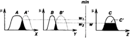
A fuzzy if-then rule with two antecedents is usually written as “if x is

A

and g is B then z is C.” The corresponding problem for approximate reasoning is expressed as

premise 1 (fact): premise 2 (rule): consequence (conclusion): z is C’ x is

A’

and y is

B’

if z is A I and y is B1 then z is C1

The fuzzy rule in premise 2 above can be put into the simpler fomi “ A x B -+ C.” Intuitively, this fuzzy rule can be transformed into a ternary fuzzy relation R, which is specified by the following MF:

And the resulting C’ is expressed as

C’ = (A’ x B’) o ( A x B -+ C ) .

Thus

where w1 is the degree of match between A and A‘; w2 is the degree of match between B and B’; and w1 A 202 is called the firing strength or degree of fu&Elment of this fuzzy rule. A graphic interpretation is shown in Fig. 9, where the MF of the resulting C’ is equal to the

MF of C clipped by the firing strength w , w = w1 A w2. The generalization to more than two antecedents is straightforward.

2) Multiple Rules with Multiple Antecedents: The interpretation of multiple rules is usually taken as the union of the fuzzy relations corresponding to the fuzzy rules. For instance, given the following fact and rules:

I

X

’4

Fig. 10. Fuzzy reasoning for multiple rules with multiple an- tecedents. premise 1 (fact): premise 2 (rule 1): premise 3 (rule 2 ) : x is A’ and y is B’ if z is A1 and y is B1 then z is C1 if z is A2 and y is Bz then z is C, consequence (conclusion): z is C’

we can employ the fuzzy reasoning shown in Fig. 10 as an inference procedure to derive the resulting output fuzzy set C’.

To verify this inference procedure, let RI = A1 x B1 --+ C1 and R2 = A2 x B2 -+ ( 3 2 . Since the max-min composition operator o is distributive over the U operator, it follows that

C’ = (A’ x B’) o (RI U R2)

= [(A’ x B’) o R I ] U

[(A‘

x B‘) o Rz]

=c;

U

c;

(17)

where Ci and Ch are the inferred fuzzy sets for rule 1

and 2, respectively. Fig. 10 shows graphically the operation of fuzzy reasoning for multiple rules with multiple antecedents.

When a given fuzzy rule assumes the form “if x is A or y is B then z is C,” then firing strength is given as the maximum of degree of match on the antecedent part for a given condition. This fuzzy rule is equivalent to the union of the two fuzzy rules “if z is A then z is C” and “if 7~ is B then z is C” if and only if the max-min composition is adopted.

D.

Fuzzy Models (Fuzzy Inference Systems)

The Fuzzy inference system is a popular computing frame- work based on the concepts of fuzzy set theory, fuzzy if-then rules, and fuzzy reasoning. It has been successfully applied in fields such as automatic control, data classification, decision analysis, expert systems, and computer vision. Because of its multi-disciplinary nature, the fuzzy inference system is known by a number of names, such

(8)

min

I

X

I

Y 0x z Fig. 11.

for fuzzy AND and OR operators, respectively.

The Mamdani fuzzy inference system using min and max

as “fuzzy-rule-based system,” “fuzzy expert system” (381, “fuzzy model” [89], [96], “fuzzy associative memory” [48], “fuzzy logic controller” [50], [51], 1611, and simply (and ambiguously) “fuzzy system.”

The basic structure of a fuzzy inference system consists of three conceptual components: a rule base, which contains a selection of fuzzy rules, a database or dictionary, which defines the membership functions used in the fuzzy rules, and a reasoning mechanism, which performs the inference procedure (usually the fuzzy reasoning introduced earlier) upon the rules and a given condition to derive a reasonable output or conclusion.

In what follows, we will first introduce three types of the most commonly used fuzzy inference systems. Then we will introduce three ways of partitioning the input space for any type of fuzzy inference system. Last, we will address briefly the features and the problems of fuzzy modeling, which is concemed with the construction of a fuzzy inference system for modeling a specific target system.

1 ) Mamdani Fuzzy Model: The Mamdani fuzzy model [61] was proposed as the very first attempt to control a steam engine and boiler combination by a set of linguistic control rules obtained from experienced human operators. Fig. 11 is an illustration of how a two-rule fuzzy inference system of the Mamdani type derives the overall output z

when subjected to two crisp inputs x and y.

If we adopt product and max as our choice for the fuzzy AND and OR operators, respectively, and use max-product composition instead of the original max-min composition, then the resulting fuzzy reasoning is shown in Fig. 12, where the inferred output of each rule is a fuzzy set scaled down by its firing strength via the algebraic product. Though this type of fuzzy reasoning was not employed in Mamdani’s original paper, it has often been used in the literature. Other variations are possible if we have different choices of fuzzy AND (T-norm) and OR (T-

conorm) operators.

I

X

I

Y ax I 1. z Fig. 12. The Mamdani f u u y inferexe system using p r ~ d t r c t

and max for fuzzy AND dnd OR operaLor5, re\pectively

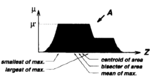
In Mamdani’s application [61], two fuzzy inference systems were used as two controllers to generate the heat input to the boiler and throttle opening of the engine cylinder, respectively, in order to regulate the steam pressure in the boiler and the speed of the engine. Since the plant takes only crisp values as inputs, we have to use a defuzzifier to convert a fuzzy set to a crisp value. DefuzziJication refers to the way a crisp value is extracted from a fuzzy set as a representative value. The most frequently used defuzzification strategy is the centroid of area. which is defined as

where p c / ( x ) is the aggregated output MF. This formula is reminiscent of the calculation of expecled values in probability distributions. Other defuzzification strategies arise for specific applications, which includes bisector of area, mean of maximum, largest of maximum, and smallest of maximum, and so on. Fig. 13 demonstrates these defuzzification strategies. Generally speaking, these defuzzification methods are computation intensive and there is no rigorous way to analyze them except through experiment-based studies. Other more flexible defuzzification methods can be found in [72], [79], [ I 131.

Both Figs. 11 and 12 conform to the fuzzy reasoning defined previously. In practice, however, a fuzzy inference system may have certain reasoning mechanisms that do not follow the strict definition of the compositional rule of inference. For instance, one might use either min or product for computing firing strengths and/or qualified rule outputs. Another variation is to use pointwise summation (sum) instead of max in the standard fuzzy reasoning, though sum is not really a fuzzy OR operators. An advantage of this sum-product composition [48] is that the final crisp output

(9)

-

centroid of area blaectw of area smallest of max.

&

J

- mean ofmer. largest of max.

Fig. 13. Various defuzzification schemes for obtdining a crisp output.

via centroid defuzzification is equal to the weighted average of each rule’s crisp output, where the weighting factor for a rule is equal to its firing strength multiplied by the area of the rule’s output MF, and the crisp output of a rule is equal to the centroid defuzzified value of its output MF. This reduces the computation burden if we can obtain the area and the centroid of each output MF in advance.

2) Sugeno Fuzzy Model: The Sugeno fuzzy model (also known as the TSK fuzzy model) was proposed by Takagi, Sugeno, and Kang [89], [96] in an effort to develop a systematic approach to generating fuzzy rules from a given input-output data set. A typical fuzzy rule in a Sugeno fuzzy model has the form

if z is A and y is B then z = f ( z , y)

where A and B are fuzzy sets in the antecedent, while

z = f(z, y) is a crisp function in the consequent. Usually

f ( z , y) is a polynomial in the input variables z and y, but it can be any function as long as it can appropriately describe the output of the system within the fuzzy region specified by the antecedent of the rule. When f(z, y) is a first-order polynomial, the resulting fuzzy inference system is called a first-order Sugeno fuzzy model, which was originally proposed in [89], [96]. When f is a constant, we then have a

zero-order Sugeno fuzzy model, which can be viewed either as a special case of the Mamdani fuzzy inference system, in which each rule’s consequent is specified by a fuzzy singleton (or a predefuzzified consequent), or a special case of the Tsukamoto fuzzy model (to be introduce later), in which each rule’s consequent is specified by an MF of a step function crossing at the constant. Moreover, a zero-order Sugeno fuzzy model is functionally equivalent to a radial basis function network under certain minor constraints [33]. It should be pointed out that the output of a zero-order Sugeno model is a smooth function of its input variables as long as the neighboring MF’s in the premise have enough overlap. In other words, the overlap of MF’s in the consequent does not have a decisive effect on the smoothness of the interpolation; it is the overlap of the MF’s in the premise that determines the smoothness of the resulting input-output behavior.

Fig. 14 shows the fuzzy reasoning procedure for a first- order Sugeno fuzzy model. Since each rule has a crips output, the overall output is obtained via weighted average and thus the time-consuming procedure of defuzzification is avoided. In practice, sometimes the weighted average

X Y

I

d g h t d s v e r a g e

1 =-

w t z i + w a z r I*l + wa

Fig. 14. The Sugeno fuzzy model.

mi” cv

I I

X Y

Fig. 15. The Tsukamoto fuzzy model.

operator is replaced with the weighted sum operator (that is, z = wlzl

+

w2z2 in Fig. 14) in order to further reduce computation load, especially in training a fuzzy inference system. However, this simplification could lead to the loss

of MF linguistic meanings unless the sum of firing strengths (that is,

E,

w,) is close to unity.

3 ) Tsukamoto Fuzzy Model: In the Tsukamoto fuzzy m d -

els [99l, the consequent of each fuzzy if-then rule is represented by a fuzzy set with a monotonical MF, as shown in Fig. 15. As a result, the inferred output of each rule is defined as a crisp value induced by the rule’s firing strength. The overall output is taken as the weighted average of each rule’s output. Fig. 15 illustrates the whole reasoning procedure for a two-input two-rule system.

Since each rule infers a crisp output, the Tsukamoto fuzzy model aggregates each rule’s output by the method of weighted average and thus also avoids the time-consuming process of defuzzification.

4 ) Partition Styles for Fuuy Models: By now it should be clear that the spirit of fuzzy inference systems resembles that of “divide and conquer”-the antecedents of fuzzy rules partition the input space into a number of local fuzzy regions, while the consequents describe the behavior within a given region via various constituents. The consequent constituent could be an output MF (Mamdani and Tsukamoto fuzzy models), a constant (zero-order Sugeno model), or a linear equation (first-order Sugeno model). Different consequent constituents result in different fuzzy

inference systems, but their antecedents are always the

(10)

(a) (b)

Various methods for partitioning the input space: (a) grid partition; (b) tree partition; Fig. 16.

(c) scatter partition.

same. Therefore the following discussion of methods of partitioning input spaces to form the antecedents of fuzzy rules is applicable to all three types of fuzzy inference systems.

Grid Partition: Fig. 16(a) illustrates a typical grid partition in a two-dimensional input space. This partition method is often chosen in designing a fuzzy controller, which usually involves only several state variables as the inputs to the controller. This partition strategy needs only a small number of MF’s for each input. However, it encounters problems when we have a moderately large number of inputs. For instance, a fuzzy model with 10 inputs and two MF’s on each input would result in 2’O = 1024 fuzzy if-then rules, which is prohibitively large. This problem, usually referred to as the curse of dimensionality, can be alleviated by the other partition strategies introduced below.

Tree Partition: Fig. 16(b) shows a typical tree partition, in which each region can be uniquely specified along a corresponding decision tree. The tree partition relieves the problem of an exponential increase in the number of rules. However, more MF’s for each input are needed to define these fuzzy regions, and these MF’s do not usually bear clear linguistic meanings such as “small,” “big,” and so on.

Scatter Partition: As shown in Fig. 16(c), by covering a subset of the whole input space that characterizes a region of possible occurrence of the input vectors, the scatter partition can also limit the number of rules to a reasonable amount.

5 ) Neuro-Fuzzy Modeling: The process for constructing a fuzzy inference system is usually called “fuzzy modeling,” which has the following features:

Due to the rule structure of a fuzzy inference system, it is easy to incorporate human expertise about the target system directly into the modeling process. Namely, fuzzy modeling takes advantage of domain knowledge that might not be easily or directly employed in other modeling approaches.

When the input-output data of a system to be modeled is available, conventional system identification techniques can be used for fuzzy modeling. In other words, the use of numerical data also plays an important role in fuzzy modeling, just as in other mathematical modeling methods.

common practice is to use domain knowledge for structure determination (that is. determine relevant inputs, number of MF’s for each input, number of rules, types of fuzzy models, and so on) and numerical data for parameter identification (that is, identify the values of parameters that can generate best the performance). In particular, the term neuro-fuzzy modeling refers to the way of applying various learning techniques developed in the neural network literature to fuzzy inference systems. In the subsequent sections, we will apply the concept of the adaptive network, which is a generalization of the common back-propagation neural network, to tackle the parameter identification problem in a fuzzy inference system.

111. ADAPTIVE NETWORKS

This section describes the architectures and learning procedures of adaptive networks, which are a superset of all kinds of neural network paradigms with supervised learning capability. In particular, we shall address two of the most popular network paradigms adopted in the neural network literature: the back-propagation neural network (BPNN) and the radial basis function network (RBFN). Other network paradigms that can be interpreted as a set of fuzzy if-then rules are described in the next section.

A. Architecture

As the name implies, an adaprive nehvork (Fig. 17) is a network structure whose overall input-output behavior is determined by the values of a collection of modifiable parameters. More specifically, the configuration of an adaptive network is composed of a set of nodes connected through directed links, where each node is a process unit that performs a static node function on its incoming signals to generate a single node output and each link specifies the

(11)

t

Inputlayer layer 1 layer2 layer3 (WOHlt Fig. 17.

tion.

A feedforward adaptive network in layered representa-

direction of signal flow from one node to another. Usually a node function is a parameterized function with modifiable parameters; by changing these parameters, we are actually changing the node function as well as the overall behavior of the adaptive network.

In the most general case, an adaptive network is hetero- geneous and each node may have a different node function. Also remember that each link in an adaptive network are merely used to specify the propagation direction of a node’s output; generally there are no weights or parameters associated with links. Fig. 17 shows a typical adaptive network with two inputs and two outputs.

The parameters of an adaptive network are distributed into the network’s nodes, so each node has a local parameter set. The union of these local parameter sets is the network’s overall parameter set. If a node’s parameter set is nonempty, then its node function depends on the parameter values; we use a square to represent this kind of adaptive node. On the other hand, if a node has an empty parameter set, then its function is fixed; we use a circle to denote this type of fixed node. Adaptive networks are generally classified into two categories on the basis of the type of connections they have: feedforward and recurrent types. The adaptive network shown in Fig. 17 is a feedfonvard network, since the output of each node propagates from the input side (left) to the output side (right) unanimously. If there is a feedback link that forms a circular path in a network, then the network is a recurrent network; Fig. 18 is an example. (From the viewpoint of graph theory, a feedforward network is represented by an acyclic directed graph which contains no directed cycles, while a recurrent network always contains at least one directed cycle.)

In the layered representation of the feedforward adaptive network in Fig. 17, there are no links between nodes in the same layer and outputs of nodes in a specific layer are always connected to nodes in succeeding layers. This representation is usually preferred because of its modularity, in that nodes in the same layer have the same functionality or generate the same level of abstraction about input vectors.

Another representation of feedfonvard networks is the topological ordering representation, which labels the nodes in an ordered sequence 1, 2, 3,

. . .

,

such that there are no links from node i to node j whenever i

2

j. Fig. 19

U

Fig. 18. A recurrent adaptive network

is the topological ordering representation of the network in Fig. 17. This representation is less modular than the layer representation, but it facilitates the formulation of the leaming rule, as will be seen in the next section. (Note that the topological ordering representation is in fact a special case of the layered representation, with one node per layer.) Conceptually, a feedfonvard adaptive network is actually a static mapping between its input and output spaces; this mapping may be either a simple linear relationship or a highly nonlinear one, depending on the structure (node arrangement and connections, and so on) for the network and the function for each node. Here our aim is to construct a network for achieving a desired nonlinear mapping that is regulated by a data set consisting of a number of desired input-output pairs of a target system. This data set is usually called the training data set and the procedure we follow in adjusting the parameters to improve the performance of the network are often referred to as the learning rule or learning algorithm. Usually an adaptive network’s performance is measured as the discrepancy between the desired output and the network’s output under the same input conditions. This discrepancy is called the error measure and it can assume different forms for different applications. Generally speaking, a leaming rule is derived by applying a specific optimization technique to a given error measure.

Before introducing a basic learning algorithm for adaptive networks, we shall present several examples of adaptive networks.

Example 3: An Adaptive Network with a Single Linear Node: Fig. 20 is an adaptive network with a single node specified by

where x1 and z2are inputs and a l . a2, and a.3 are modifiable parameters. Obviously this function defines a plane in 2 1 - :c2 - 5 3 space, and by setting appropriate values for the parameters, we can place this plane arbitrarily. By adopting the squared error as the error measure for this network, we can identify the optimal parameters via the Example 4: A Building Block for the Perceptron or the Back-Propagation Neural Network: If we add another node to let the output of the adaptive network in Fig. 20 have only two values 0 and 1, then the nonlinear network shown linear least-squares estimation method.

0

(12)

Fig. 19. A fecdforward adaptive network in topological ordering representation.

Fig. 20. A linear single-node adaptive network.

Fig. 21. A nonlinear single-node adaptive network.

in Fig. 21 is obtained. Specifically, the node outputs are expressed as

and

1 if 2 3 2 0 0 if z3

<

0 3:4 = f4(3:3) =

where f 3 is a linearly parameterized function and f 4 is a

step function which maps -c3 to either 0 or 1. The overall function of this network can be viewed as a linear classi$er: the first node forms a decision boundary as a straight line in 11'1 - x2 space, and the second node indicates which half plane the input vector ( T I . ,c2) resides in. Obviously we can form an equivalent network with a single node whose function is the composition of f3 and f 4 ; the resulting node is the building block of the classical perceptron.

Since the step function is discontinuous at one point and flat at all the other points, it is not suitable for learning procedures based on gradient descent. One way to get around this difficulty is to use the sigmoid function:

which is a continuous and differentiable approximation to the step function. The composition of f3 and this differentiable f 4 is the building block for the back-propagation

0

neural network in the following example.

.

U

f

t

f

layer 0 layer 1 layer 2

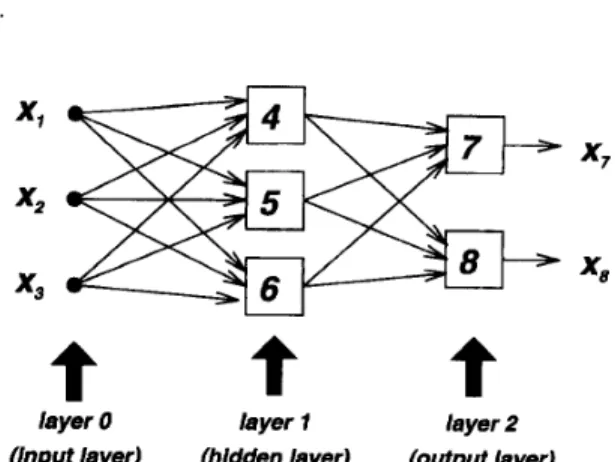
(Input layer) (hidden layer) (output layer) Fig. 22. A 3-3-2 neural network.

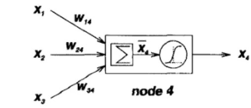
Example 5: A Back-Propagation Neurul Network: Fig. 22 is a typical architecture for a back-propagation neural network with three inputs, two outputs, and three hidden nodes that do not connect directly to either inputs or outputs. (The term back-propagation refers to the way the learning procedure is performed, that is, by propagating gradient information from the network's outputs to its inputs; details on this are to be introduced next.) Each node in a network of this kind has the same node function, which is the composition of a linear f 3 and a sigmoidal fi in

Example 4. For instance, the node function of node 7 in Fig. 22 is

where x4, .c5, and :E6 are outputs from nodes 4, 5 , and

6, respectively, and ( 7 ~ 4 , ~ : 2 1 1 5 , ~ . ' u I ~ , J . t:.} is the parameter

set. Usually we view wi;j as the weight associated with the link connecting node i and j and t j as the threshold associated with node j . However, it should be noted that this weight-link association is only valid in this type of network. In general, a link only indicates the signal flow direction and, the causal relationship between connected nodes, as will be shown in other types of adaptive networks in the subsequent development. A more detailed discussion about the structure and learning rules of the artificial neural

0

network will be presented later.

(13)

xo,

1

xo.2

t

_t

t

layer 0 layer 1 layer 2 layer 3

(a)

n

0 . (b) Fig. 23. sentation

Our notational conventions: (a) layered representation; (b) topological ordering repre-

B. Back-Propagation Learning Rule

The central part of a learning rule for an adaptive network concerns how to recursively obtain a gradient vector in which each element is defined as the derivative of an error measure with respect to a parameter. This is done by means of the chain rule, and the method is generally referred to as the "back-propagation learning rule" because the gradient vector is calculated in the direction opposite to the flow of the output of each node. Details follow below.

Suppose that a given feedforward adaptive network in the layered representation has L layers and layer 1(1 = 0,

1, .

. . .

L ; I = 0 represents the input layer) has N ( l ) nodes. Then the output and function of node

i (i

= 1, . . .

,

N ( l ) )

of layer 1 can be represented as xl.? and .fl.z, respectively, as shown in Fig. 23(a). Without loss of generality, we assume there are no jumping links, that is, links connecting nonconsecutive layers. Since the output of a node depends on the incoming signals and the parameter set of the node, we have the following general expression for the node function fl,?:

5 1 , z = ~ / , ~ ( x / - l , l , . . . ~ l - l , ~ ( l - ~ ) , a , / ? , ~ , . . . ) (19)

where a ,

/?,

7 , etc., are the parameters pertaining to this node.

Assuming the given training data set has P entries, we can define an error measure for the p th (1

5

p

5

P ) entry of the training data as the sum of squared errors:

where d k is the kth component of the pth desired output vector and X L , k is the kth component of the actual output vector produced by presenting the pth input vector to the network. (For notational simplicity, we omit the subscript p for both d k and X L , ~ . ) Obviously, when Ep is equal to zero, the network is able to reproduce exactly the desired output vector in the pth training data pair. Thus our task here is to minimize an overall error measure, which is defined as Remember that the definition of E p in (20) is not universal; other definitions of E p are possible for specific situations or applications. Therefore we shall avoid using an explicit expression for the error measure E p in order to emphasize the generality. In addition, we assume that E p

depends on the output nodes only; more general situations will be discussed below.

To use the gradient method to minimize the error measure, first we have to obtain the gradient vector. Before calculating the gradient vector, we should observe that

P

E =

C,=lEP.

/changein*rchangeintheourput/

parametera of node containing Q:

change in the output change in the output

*

[

F

l

*

F

l

where the arrows

*

indicate causal relationships. In other words, a small change in a parameter a will affect the

(14)

The error signal for the ith output node (at layer L ) can be calculated directly:

Fig. 24. text for details).

Ordered derivatives and ordinary partial derivatives (see

output of the node containing a ; this in turn will affect the

output of the final layer and thus the error measure. There- fore the basic concept in calculating the gradient vector of the parameters is to pass a form of derivative information starting from the output layer and going backward layer by layer until the input layer is reached.

To facilitate the discussion, we define the error signal

F L , ~ as the derivative of the error measure Ep with respect

to the output of node i in layer 1, taking both direct and indirect paths into consideration. In symbols,

This expression was called the “ordered derivative” by Werbos [107]. The difference between the ordered derivative and the ordinary partial derivative lies in the way we view the function to be differentiated. For an internal node output . c ~ , ~ (where 1

#

L ) , the partial derivative

(?lEP/axl,&) is equal to zero, since E p does not depend on ~ 1directly. However, it is obvious that , ~ E p does depend on ~ 1 indirectly, since a change in , ~ ~ 1 will propagate , ~ through indirect paths to the output layer and thus produce a corresponding change in the value of E p . Therefore can be viewed as the ratio of these two changes when they are made infinitesimal. The following example demonstrates the difference between the ordered derivative and the ordinary partial derivative.

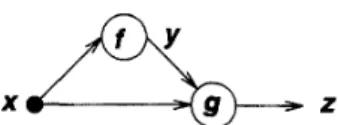
Example 6: Ordered Derivatives and Ordinary Partial Derivatives: Consider the simple adaptive network shown in Fig. 24, where z is a function of

x

and y, and y is in turn a function of x:

Y =

f(x.).

{

2 = d G Y ) .

For the ordinary partial derivative ( a z / d z ) , we assume that all the other input variables (in this case, y) are constant:

ax

.

In other words, we assume the direct inputs x and y are independent, without paying attention to the fact that y is actually a function of

x.

For the ordered derivative, we take this indirect causal relationship into consideration:

az - a g ( ~ , y >

-~ -

a+z

- _-

a d z , f

(.)I

i ) X d X

Therefore the ordered derivative takes into consideration both the direct and indirect paths that lead to the causal

relationship.

0

This is equal to EL,^ = - 2 ( 4 - Z L , ~ ) if Ep is defined as in

(20). For the internal (nonoutput) node at the ith position of layer 1, the error signal can be derived by the chain rule:

error signal error signal at layer 1+1

at layer 1

where 0

5

1

5

L- 1. That is, the error signal of an internal node at layer 1 can be expressed as a linear combination of the error signal of the nodes at layer 1+ I . Therefore for any I and .i (0

5 I

5

L and 1

5

i

5

N ( l ) ) , we can find = ( d + E p / 3 x l , z ) by first applying (22) once to get error signals at the output layer, and then applying

(23) iteratively until we reach the desired layer 1. Since the error signals are obtained sequentially from the output layer back to the input layer, this learning paradigm is called the “back-propagation” learning rule by Rumelhart, Hinton, and Williams [78].

The gradient vector is defined as the derivative of the error measure with respect to each parameter, so we have to apply the chain rule again to find the gradient vector. If

a is a parameter of the ith node at layer