國 立 交 通 大 學
電 機 與 控 制 工 程 研 究 所
碩 士 論 文
Nearest Neighbor 演算法處理符號性質資料的
分類及其於蛋白質二級結構預測的應用
Nearest Neighbor Algorithm for Symbolic Data Set
Classification and Its Application in Protein
Secondary Structure Prediction
研 究 生 : 黃 培 倉
指 導 教 授: 張 志 永
Nearest Neighbor 演算法處理符號性質資料的分類及其於蛋白質二
級結構預測的應用
Nearest Neighbor Algorithm for Symbolic Data Set Classification and
Its Application in Protein Secondary Structure Prediction
學 生 : 黃培倉 Student : Pei-Chang Chen
指導教授 : 張志永 Advisor : Jyh-Yeong Chang
國立交通大學
電機與控制工程學系
碩士論文
A Thesis
Submitted to Department of Electrical and Control Engineering
College of Electrical Engineering and Computer Science
National Chiao Tung University
in Partial Fulfillment of the Requirements
for the Degree of Master in
Electrical and Control Engineering
July 2005
Hsinchu, Taiwan, Republic of China
Nearest Neighbor 演算法處理符號性質資料的分類及其於
蛋白質二級結構預測的應用
學生:黃培倉 指導教授:張志永博士 國立交通大學電機與控制工程研究所摘要
蛋白質在生物體中一直扮演著很重要的角色且蛋白質被發現的數量及其結 構逐年增加。隨著蛋白質的應用越來越廣泛,待解決的課題也就越來越多。例如: 蛋 白 質 二 級 結 構 預 測 問 題 、 蛋 白 質 摺 疊 預 測 問 題(Protein folding prediction problem)、蛋白質投射問題(Protein mapping problem)等。目前在蛋白質相關問題的解決上,科學家都是利用 X 光繞射以及核磁共振(NMR)來取得實驗結果。這 些方法雖然正確率高,但是相對地所要花費的時間及成本是相當高的。因此利用 電腦科學中的機器學習(Machine learning)演算法來預測這些問題相信是能夠有 效降低實驗成本的。 本篇論文,我們利用了 Nearest Neighbor 演算法僅針對了蛋白質二級結構預 測問題進行了實驗。正如我們大家所知道的,每一種蛋白質序列皆是由20 種不 同的胺基酸(Amino acid)所組成,而每一種胺基酸都可視為一個符號(Symbol)。 在過去,Nearest Neighbor 演算法通常是用來處理資料屬性全部是數值的例子。
在這樣的屬性當中,這些事例(Instance)都是被視為點,而且彼此之間的距離都適 用於歐幾里得距離。然而在符號屬性的領域當中,處理符號是利用特定的距離表
以產生事例之間的實質距離。我們所使用的距離是由 Stanfill 和 Waltz 所提出的
Value Difference Metric 表來定義出兩個符號間的實質距離。基於 Value Difference Metric 表的架構下,我們提出了兩個不同的判定法則來預測蛋白質二級結構。除 此之外,我們也研究且實做了目前常用的一種預測法-PSIPRED。最後,我們試
著將我們所用的兩種演算法和PSIPRED 做結合,並朝向著混合後的準確率能夠
Nearest Neighbor Algorithm for Symbolic Data Set
Classification and Its Application in Protein Secondary
Structure Prediction
STUDENT: PEI-CHANG HUANG ADVISOR: JYH-YEONG CHANG
Institute of Electrical and Control Engineering National Chiao-Tung University
Abstract
Proteins have been played an important role in a creature and the number of proteins and their structures have been increased with years. Since protein applications are more widely used, there will be a lot of problems to be solved. For example, there are protein secondary structure prediction problem, protein folding problem, protein mapping problem and so on. Nowadays, scientists use X-ray diffraction or nuclear magnetic resonance(NMR) to solve the protein problem. Even though chemical experiments can achieve high accuracy, it in the mean time incurs high costs and long time to solve the protein problems. Therefore, we think that it is possible to reduce the time and the costs mentioned above by using machine learning algorithm in computer science.
In this thesis, we make an experiment on protein secondary structure prediction problem using nearest neighbor algorithm. As all we know, every protein is consisted of twenty kinds of amino acid. Every kind of amino acid can be regarded as a symbol. In the past, nearest neighbor algorithms for learning from examples have worked well in domains in which all features had numeric values. In such domains, the examples can be treated as points and distance metrics can be exploited using Euclidean distance. However, the nearest neighbor algorithm used for the symbolic domain calculates distance tables that allow it to produce real-valued distances between instances. The method we used is proposed by Stanfill and Waltz and is called Value Difference Metric table, we propose two different algorithms to predict protein secondary structure. Besides, we also study and implement PSIPRED, a common method of the protein secondary structure prediction in recent years. Finally, we try to combine our two different algorithms with PSIPRED and make an effort on elevating the accuracy in predicting protein secondary structure.
ACKNOWLEDGEMENT
I would like to express my sincere appreciation to my advisor, Dr. Jyh-Yeong Chang. Without his patient guidance and inspiration during the two years, it is impossible for me to overcome the obstacles and complete the thesis. In addition, I am thankful to all my lab members for their discussion and suggestion.
Finally, I would like to express my deepest gratitude to my parents. Without their strong support and encouragement, I could not go through the two years.
Content
ABSTRACT (CHINESE)……….i
ABSTRACT (ENGLISH)...………ii
ACKNOWLEDGEMENT.…………...………...iii
Chapter 1. Introduction………...
11.1 Motivation and The Background of This Research………1
1.2 Brief Introduction to The Protein Secondary Structure………...2
1.3 Introduction to Machine Learning and Nearest Neighbor Algorithms for Learning with Continuous Features……….6
1.4 Thesis Outline……….8
Chapter 2. Nearest Neighbor Algorithm for Symbolic Data…………9
2.1 Overlap Metric………9
2.2 Value Difference Metric………...10
2.3 Distances between Protein Symbols Using VDM Table………..13
Chapter 3. Protein Secondary Structure Prediction………...22
3.2 The VDM Table Method with Nearest Neighbor Majority Vote.………….25
3.3 The VDM Table Method with Nearest Neighbor Balanced Prediction……27
3.4 Fusion Method………..………28
3.4.1 Majority Vote Based on the Global Confidence Value…..………...…28
3.4.2 Majority Vote Based on the Local Confidence Value………30
Chapter 4. Experiment and Simulation Results………..32
4.1 Introduction to Data Sets………..………32
4.2 Simulation Results of VDM Method with Nearest Neighbor Majority Vote ………34
4.3 Simulation Results of VDM Method with Nearest Neighbor Balanced Prediction……….39
4.4 Simulation Results of PSIPRED………44
4.5 Simulation Results of Fusion Method………...46
4.5.1 Results of Majority Vote Based on the Global Confidence Value……….46
4.5.2 Results of Majority Vote Based on the Local Confidence Value………...52
4.6 Accuracy Comparison and Comments………..59
Chapter 5. Conclusion………61
List of Figures
Fig. 1.1. The α-helix structure…...………..…..3
Fig. 1.2. The Ramachandarn Plot………...…………...3
Fig. 1.3. The Anti-parallel β-sheet……..………...4
Fig. 1.4. The Parallel β-sheet……….………..5
Fig. 1.5. Two hairpin loops between three anti-parallel β-strands ……….5
Fig. 1.6. Simple 2-D case, each instance is described only by two values...7
Fig. 2.1. The distance between instances X and Y……...………13
Fig. 3.1. The overall flowchart of PSIPRED………...24
Fig. 3.2. The testing and the training data………...26
Fig. 3.3. The VDM tables constructed by the training data………26
Fig. 4.1. The accuracy plot of 120 proteins with VDM_100-NN_MV method…..35
Fig. 4.2. The accuracy plot of 120 proteins with VDM_150-NN_MV method…..36
Fig. 4.3. The accuracy plot of 120 proteins with VDM_200-NN_MV method…..37
Fig. 4.4. The accuracy plot of 120 proteins with VDM_100-NN_BP method…..40
Fig. 4.5. The accuracy plot of 120 proteins with VDM_150-NN_BP method……41
Fig. 4.6. The accuracy plot of 120 proteins with VDM_200-NN_BP method……42
Fig. 4.7. The accuracy plot of 120 proteins with PSIPRED method………45
Fig. 4.8. The accuracy plot of 120 proteins with Fusion 1 method………47
Fig. 4.9. The accuracy plot of 120 proteins with Fusion 2 method……….49
Fig. 4.10. The accuracy plot of 120 proteins with Fusion 3 method……….51
Fig. 4.11. The accuracy plot of 120 proteins with Fusion 4 method……….53
Fig. 4.12. The accuracy plot of 120 proteins with Fusion 5 method……….55
List of Tables
Table 2.1. Number of occurrences of each symbol value to each class…...11
Table 2.2. Value Difference Metric Table………...12
Table 2.3. Occurrence table of the example for Feature 1……..……….16
Table 2.4. Occurrence table of 31755 residues for Feature 1………...17
Table 2.5. Global VDM table of 31755 residues for Feature 1 ………..18
Table 3.1. The change of distribution ratio corresponding to the original ratio…..27
Table 3.2. The individual accuracy of three classes with different methods……..29
Table 3.3. The class labels predicted by three different methods………...29
Table 3.4. The total global confidence value table for each position………..30
Table 3.5. The local confidence value for three classes by different method…31 Table 4.1. The database of this research……….33
Table 4.2. The accuracy of 120 proteins with VDM_100-NN_MV method……35
Table 4.3. The accuracy of 120 proteins with VDM_150-NN_MV method……36
Table 4.4. The accuracy of 120 proteins with VDM_200-NN_MV method……37
Table 4.5. The average accuracies and standard deviations of 120 proteins…….38
Table 4.6. The average accuracies for three classes with different No. of Neighbors………...38
Table 4.7. The accuracy of 120 proteins with VDM_100-NN_BP method……..39
Table 4.8. The accuracy of 120 proteins with VDM_150-NN_BP method…...41
Table 4.9. The accuracy of 120 proteins with VDM_200-NN_BP method……42
Table 4.10. The average accuracies and standard deviations of 120 proteins…….43
Table 4.11. The average accuracies for three classes with different No. of Neighbors………...43
Table 4.12. The accuracy of 120 proteins with PSIPRED………...44 Table 4.13. The average accuracy and standard deviation of 120 proteins……...45 Table 4.14. The average accuracy of PSIPRED for three classes………...45 Table 4.15. The global confidence values of three classes for three methods (Fusion 1)……….46 Table 4.16. The accuracy of 120 proteins for Fusion 1……….47 Table 4.17. The average accuracy and standard deviation of 120 proteins………48 Table 4.18. The global confidence values of three classes for three methods (Fusion 2)……….48 Table 4.19. The accuracy of 120 proteins for Fusion 2……….49 Table 4.20. The average accuracy and standard deviation of 120 proteins……50 Table 4.21. The global confidence values of three classes for three methods (Fusion 3)………...50 Table 4.22. The accuracy of 120 proteins for Fusion 3……….51 Table 4.23. The average accuracy and standard deviation of 120 proteins……52 Table 4.24. The accuracy of 120 proteins for Fusion 4……….53 Table 4.25. The average accuracy and standard deviation of 120 proteins……54 Table 4.26. The accuracy of 120 proteins for Fusion 5……….55 Table 4.27. The average accuracy and standard deviation of 120 proteins……56 Table 4.28. The accuracy of 120 proteins for Fusion 6……….57 Table 4.29. The average accuracy and standard deviation of 120 proteins……58 Table 4.30 The accuracy ranking of 13 approaches………..59
Chapter 1. Introduction
1.1 Motivation and The Background of This Research
The number of proteins and its structure has been increased in recent years. Since
protein applications are more widely used, there will be a lot of problems to be solved. For example, there are protein secondary structure prediction problems [1]–[4], protein fold recognition problems [5], [6], protein mapping problems and so on. Nowadays, scientists use X-ray diffraction or nuclear magnetic resonance (NMR) to solve the protein structure problems. Even though chemical experiments can achieve high accuracy, they in the mean time incur high costs and long time to solve the protein problems. Therefore, we believe that using machine learning methods in the computer science field is promising, because it not only reduces the time and the costs but also maintains the accuracy.
In this thesis, we make an algorithmic prediction on the protein secondary structure prediction problem using nearest neighbor algorithm [7]. Predicting the secondary structure of a protein (α-helix, β-sheet and coil) is an important step towards elucidating its three dimensional structure and its function. In the past, nearest neighbor algorithms via learning from examples have worked well in domains in which all features had numeric values. In such domains, the examples can be treated as points and distance metrics can be exploited, using Euclidean distance for example. However, when the feature values are symbolic, a more sophisticated treatment of the feature space is required. The nearest neighbor algorithm used for the symbolic feature space needs to construct the distance table among symbols. From it, we can calculate real-valued distances between instances. As all we know, every
protein sequence is consisted of twenty kinds of amino acid, and every kind of amino acid can be regarded as a symbol. Under this condition, the protein secondary structure prediction problem has the symbolic feature space. The method we will adopt is proposed by Stanfill and Waltz [8] and further refined by Cost and Salzberg [9], called Value Difference Metric (VDM) table. Based on the construction of VDM table, we propose two different algorithms to predict the protein secondary structure. Besides, we also study and implement Position Specific Iterated Prediction (PSIPRED) [10], [11], a common method of the protein secondary structure prediction used in recent years. Finally, we try to combine our two different algorithms with PSIPRED and make an effort on elevating the accuracy in predicting the protein secondary structure. We will also compare the prediction accuracy of our fusion based method with PSIPRED and VDM approaches.
1.2 Brief Introduction to The Protein Secondary Structure
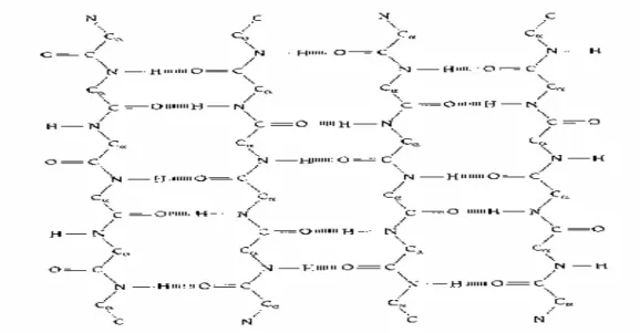
The protein secondary structure consists of local folding regularities maintained by hydrogen bonds and traditionally subdivided into three classes: α-helix, β-sheet and loop (coil) representing all the rest. The α-helix (Fig. 1.1) is the classic element of protein structure. It was first described by Linus Pauling working at the California Institute of Technology [12]. He predicted that it was a structure which would be stable and energetically favorable in proteins. Alpha helices in proteins are found when a stretch of consecutive residues all have the phi, psi angle pair approximately –85° and –50°, corresponding to the allowed region in the bottom left quadrant of the Ramachandran plot (Fig. 1.2) [13], [14].
Fig. 1.1. The α-helix structure.
Only in the α-helix are the backbone atoms properly packed to provide a stable structure. In globular proteins, the average length for α-helices is around ten residues, corresponding to three turns. The rise per residue of an α-helix is 1.5 Å along the helical axis, which corresponds to about 15 Å from one end to the other of an average α-helix.
The second major structural element found in globular proteins is the ß-sheet. This structure is built up from a combination of several regions of the polypeptide chain, in contrast to the α-helix, which is built up from one continuous region. These regions, ß-strands, are usually from five to ten residues long and are in an almost fully extended conformation with phi, psi angles within the broad structurally allowed region in the upper left quadrant of the Ramachandran plot (Fig. 1.2) [13], [14]. β-strands can interact in two ways to form a pleated sheet – parallel and anti-parallel. Each of the two forms has a distinctive pattern of hydrogen-bonding. The anti-parallel ß-sheet (Fig. 1.3) has narrowly spaced hydrogen bond pairs that alternate with widely spaced pairs. Parallel ß-sheets (Fig. 1.4) have evenly spaced hydrogen bonds that bridge the ß- strands at an angle.
Fig. 1.4. The Parallel ß-sheet.
Most protein structures are built up from combinations of secondary structure elements, α-helices and ß-strands, which are connected by loop regions of various lengths and irregular shape. The loop regions are always at the surface of protein molecules. Loop regions exposed to solvent are rich in charge and polar hydrophilic residues. Loop regions that connect two adjacent anti-parallel ß-strands are called the
hairpin loops. Short hairpin loops are usually called reverse turns or simply turns.
Fig. 1.5. Two hairpin loops between three anti-parallel ß-strands.
1.3 Introduction to Machine Learning and Nearest Neighbor Algorithms for Learning with Continuous Features
Learning is an important component of any intelligent system, whether human, animal, or machine. Machine learning [15], [16] is a field of artificial intelligence involving developing techniques to allow computers to “learn.” More specifically, it is a two-step process, which finds the common properties among a set of instances in a database and classifies them into different classes. Generally speaking, training data are analyzed by classification algorithms and then represented in the form of rules or formulas in the first step. In the second step, testing data are used to measured the accuracy of all the classification rules and formulas. If the accuracy is quite acceptable, the rules can be applied to the classification of new instance for which the class label is not known.
Machine learning algorithms can be divided into supervised and unsupervised algorithms. In supervised learning, input pattern is identified as a member of pre-defined class. In other words, the supervised learning algorithm is told to which class each training instance belongs. On the other hand, input pattern is assigned to a hitherto unknown class in unsupervised learning. This kind of learning learns the classification by searching through some common properties of the data. In case where there is no prior knowledge of classes, supervised learning can still be applied if the data has a natural clustering structure. Then a clustering algorithm has to be run first to reveal these natural groupings.
Different approaches from pattern recognition and machine learning have been used in intelligent diagnostic systems. One of the most important developments in this area is the nearest neighbor algorithm. In the past, the nearest neighbor algorithm is
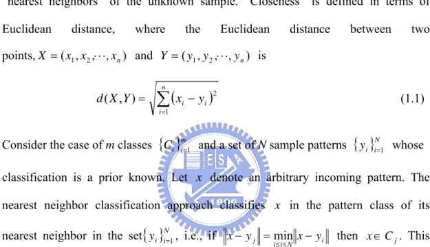
used to deal with the continuous features data. In such domains, the examples can be treated as points and distance metrics can be exploited, using Euclidean distance for instance. The training samples are described by n-dimensional numeric attributes. Each sample represents a point in an n-dimensional space. When given an unknown sample, a k-nearest neighbor classifier searches the pattern space for k training samples that are closest to the unknown sample. The k training samples are the k “nearest neighbors” of the unknown sample. “Closeness” is defined in terms of Euclidean distance, where the Euclidean distance between two points,X =(x1,x2,⋅ ⋅⋅,xn) and Y =(y1,y2,⋅ ⋅⋅,yn) is
∑
(
)
= − = n i i i y x Y X d 1 2 ) , ( (1.1)Consider the case of m classes
{ }
m and a set of N sample patterns whosei i
C =1
{ }
yi iN=1classification is a prior known. Let denote an arbitrary incoming pattern. The nearest neighbor classification approach classifies in the pattern class of its nearest neighbor in the set , i.e., if
x x
{ }
N i i y =1 i N i i j x y y x− = − ≤ ≤min then . This
scheme which is basically another type of minimum-distance classification, can be modified by considering the k nearest neighbors to and using a majority-rule type classifier. There is an example shown in Fig. 1.6.
j C x∈
x
Fig. 1.6. Simple 2-D case, each instance is described only by two values (x, y coordinates). The class is either or .
Inside the circle of Fig. 1.6, we can easily see that the class of single-NN (1-NN) is , and the class of 5-NN is , assuming that is the testing data.
1.4 Thesis Outline
The organization of this thesis is structured as follows. Chapter 1 introduces the role of machine learning, the motivation and the background of this thesis. In Chapter 2, the nearest neighbor learning with symbolic feature will be described. Then we will introduce Value Difference Metric (VDM) table and its construction method. In Chapter 3, we will first introduce PSIPRED, a common method of the protein secondary structure prediction used in recent years. Then, based on the construction of VDM table, we will propose two different methods to predict the protein secondary structure, majority vote and balanced prediction schemes. Then we will describe the combination of our two different methods with PSIPRED and elevate the accuracy by tuning the confidence values developed. In Chapter 4, the experiment of computer simulation and the results are conducted and compared to PSIPRED. Finally, the conclusion of this thesis is presented in Chapter 5.
Chapter 2. Nearest Neighbor Algorithm for Symbolic Data
2.1 Overlap Metric
The most fundamental metric that works for patterns with symbolic features is the overlap metric given in Eq. (2.1) and Eq. (2.2). In these two equations, d(X, Y) is the total distance between instances X and Y, represented by n features, and î is the distance per feature. The distance between two instances is simply the sum of the differences between n features. The k-NN algorithm with this overlap metric is called IB1 which is introduced by Aha et al [15]. Generally k is set to 1.
d(X, Y ) =P = (2.1) i=1 n ⏐ ⏐Xià Yi⏐⏐k
∑
= n i i i y x 1 ) , ( δ î(xi, yi) = abs(max iàmini xiàyi ), if 0, if 1, if ⎧ ⎪ ⎨ ⎪ ⎩ xxii =6= yyii (2.2) numeric, elseBut the overlap metric has a disadvantage that it could not decide the real intrinsic distances in symbolic domain. When the instances are not equal, it assigns a 1 of value to their distance. This assumes that each different symbolic value is equi-distant from another which leads to problems when two different values should be considered equal, and where symbolic values should have varying distances among them. However, the rule is ambiguous. The distance metric in Eq. (2.2) simply counts the number of matching or mismatching feature-values in the patterns. So overlap metric is limited to exact match between feature-values.
2.2 Value Difference Metric
Since the overlap metric could not find the degree of difference between the instances, we think that it is not a proper distance metric for calculating the distance among those instances. For this purpose, a metric was defined by Stanfill and Waltz [8] and further refined by Cost and Salzberg [9]. It is called the (Modified) Value Difference Metric, and it is a method to determine the similarity of the values of a feature by looking at co-occurrence of values with target classes. For the distance between two values, v and v of a feature, we compute the difference of the conditional distribution of the classes for these values is defined in Eq. (2.3).
1 2 Ci î(v1, v2) =P i=1 n | P (Ci| v1)à P (Ci | v2)| (2.3)
=
P
i=1 n⏐
⏐
C 1 C1ià
C2 C2i⏐
⏐
kIn this equation, and v are two possible symbols for the feature and the distance between the values is the sum of all classes. C is the number of times was classified into category i, is the total number of times value 1 (v ) occurred, and k is a constant and usually set to 1. Using Eq. (2.3), we compute a matrix of value differences for each feature in the input data. It is interesting to note that the value difference matrices computed in the experiments below are quite similar overall for different features, although they differ significantly for some value pairs.
v1 2
n 1i
v1 C1 1
The idea behind this metric is that we want to establish that values are similar if they occur with the same relative frequency for all classifications. The term
represents the likelihood that the central residue will be classified as i given that the feature in Eq. (2.3) has value . Thus we say that two values are similar if they give
C1i/C1
similar likelihood for all the possible classifications. Eq. (2.3) computes overall similarity between two values by finding the sum of the differences of these likelihoods over all classifications.
Consider the following simple example. Say that we have a pool of instances for which we only examine a single feature that takes one of three symbols: A, B and C. Assume that two classifications α and ß are possible. From the data we construct in Table 2.1. The table entries represent the number of times an instance had a given feature value and classification. From this condition we construct a table of distances as follows. The frequency of occurrence of A for class α is 60%, since there are 3 instances classified as α out of 5 instances with value A. Similarly, the frequencies of occurrence for B and C for class α are 20% and 75% respectively. The frequency of occurrence of A for class ß is 40%, and so on. In order to find the distance between A and B, we use Eq. (2.3), which yields 35− 15 + 25−45 =0.8. The complete table of distances is shown in Table 2.2. Note that we construct a difference value table for each feature.
Table 2.1. Number of occurrences of each symbol value to each class Class
Symbol Values
ë
ì
A 3 2
B 1 4
Table 2.2. Value Difference Metric Table Symbol values A B C A 0 0.8 0.3 B 0.8 0 1.1 C 0.3 1.1 0
We can find that the distance between A and C is quite small. This is due to their occurrence numbers in the α and ß are very similar. Eq. (2.3) defines geometric distance on a fixed, finite set of values. The VDM table is symmetric, and they obey the triangle inequality. We summarize these properties as follows:
i. î(a, b) > 0, a 6= b
ii. î(a, b) = î(b, a)
iii. î(a, a) = 0
iv. î(a, b) + î(b, c) õ î(a, c)
Assume that X and Y represent two instances with X being a training example and Y a testing example. The variables and y are values of the i-th feature for X
and Y, where each example has n features. Therefore, the total distance between X and
Y is the sum of all distances between i and y. The distance between X and Y is
shown in the following figure, Fig. 2.1.
xi i
Xà Y = (x1, x2, ...xn)à (y1, y2, ...yn)
(x1 à y1) + (x2à y2) + ... + (xnà yn)
VDM table of feature 1 VDM table of feature 2 VDM table of feature n
Fig. 2.1. The distance between instances X and Y.
2.3 Distances between Protein Symbols Using VDM table
As all we know, any protein sequence is consisted of 20 kinds of amino acid which are represented by 20 characters. They are Alanine (A), Cysteine (C), Aspartic acid (D), Glutamic acid (E), Phenylalanine (F), Glycine (G), Histidine (H), Isoleucine (I), Lysine (K), Leucine (L), Methionine (M), Asparagine (N), Proline (P), Glutamine (Q), Arginine (R), Serine (S), Threonine (T), Valine (V), Tryptophan (W), and Tyrosine (Y) respectively [17]. In other words, there should be 20 kinds of symbolic value for each feature. In fact, there will be 21 kinds of symbolic value for each feature in our research, and this will be explained later.
The feature number of our research is set to 13, i.e. we should make a window for every symbol (amino acid) in a protein sequence and its length is 13. This is the pre-process of our experiment. Under this condition, every symbol (amino acid) in
the protein sequence will be located in the center of the expanded window. So it both has 6 neighbors on its left-hand side and right-hand side, respectively. During the process of making windows, the fronted, i.e., the first six and the last end, i.e., the last six residues will have some unknown neighbors. We regard these unknown neighbors as another symbol “X,” and this is the reason why we will have 21 kinds of symbolic value for each feature. Let us illustrate a simple example as follows. If a protein sequence is “G K I T F Y E D R G,” then we will make a window for each symbol and they will become a 10×13 symbolic matrix which is shown as follows:
X X X X X X G K I T F Y E X X X X X G K I T F Y E D X X X X G K I T F Y E D R X X X G K I T F Y E D R G X X G K I T F Y E D R G X X G K I T F Y E D R G X X G K I T F Y E D R G X X X K I T F Y E D R G X X X X I T F Y E D R G X X X X X T F Y E D R G X X X X X X
We can see that the boldface of each row construct the original protein sequence. Each column (feature) will construct a VDM table, and each size is 21×21. In this case, we
will have 13 different VDM tables for 13 features.
Assume that the secondary structure corresponding to the original protein sequence is “α α α α ß ß ß ß l l,” we should construct the occurrence table for each feature first. We show the 10×13 symbolic matrix again by adding the secondary structure label behind each row. Therefore, it is convenient for us to check the occurrence frequency for each symbol in each class.
X X X X X X G K I T F Y E………...α X X X X X G K I T F Y E D………...α X X X X G K I T F Y E D R……….α X X X G K I T F Y E D R G……….α X X G K I T F Y E D R G X………..ß X G K I T F Y E D R G X X………..ß G K I T F Y E D R G X X X………..ß K I T F Y E D R G X X X X………..ß I T F Y E D R G X X X X X………..l T F Y E D R G X X X X X X……….l
For Feature 1 (first column), we can construct the occurrence table which is shown in Table 2.3. Note that there are many zeros in the occurrence table because the protein length of this example is too short. If the elements in a row are all zeros, we can not use Eq. (2.3) to compute the distance between two symbols in a feature.
Table 2.3. Occurrence table of the example for Feature 1
Alpha Beta Loop
A 0 0 0 C 0 0 0 D 0 0 0 E 0 0 0 F 0 0 0 G 0 1 0 H 0 0 0 I 0 0 1 K 0 1 0 L 0 0 0 M 0 0 0 N 0 0 0 P 0 0 0 Q 0 0 0 R 0 0 0 S 0 0 0 T 0 0 1 V 0 0 0 W 0 0 0 Y 0 0 0 X 4 2 0 Symbol Class
This is an example to show how an occurrence table for one feature is established. Because too many sums of the row are zeros, we can not illustrate the VDM table for 21 symbolic values for Feature 1 for this example. In our research, we make a global VDM table for 120 protein sequences in HSSP database including 31755 residues (amino acids). The occurrence table and the global VDM table of these 31755 residues for Feature 1 are shown below.
Table 2.4. Occurrence table of 31755 residues for Feature 1
Alpha Beta Loop
A 853 553 1040 C 149 164 338 D 566 428 736 E 560 415 735 F 339 241 624 G 778 743 1093 H 209 186 320 I 523 343 834 K 537 496 796 L 766 524 1166 M 209 117 266 N 447 422 666 P 409 386 740 Symbol Class
Q 358 296 502 R 376 321 550 S 591 619 973 T 559 541 896 V 601 484 1083 W 136 92 233 Y 299 271 537 X 113 184 423
Table 2.5. Global VDM table of 31755 residues for Feature 1 A C D E F G H A 0 0.238 0.043 0.043 0.186 0.116 0.113 C 0.238 0 0.197 0.197 0.105 0.202 0.143 D 0.043 0.197 0 0.009 0.186 0.074 0.070 E 0.043 0.197 0.009 0 0.177 0.083 0.070 F 0.186 0.105 0.186 0.177 0 0.200 0.141 G 0.116 0.202 0.074 0.083 0.200 0 0.059 H 0.113 0.143 0.070 0.070 0.141 0.059 0 I 0.131 0.158 0.130 0.122 0.055 0.165 0.117 K 0.110 0.168 0.067 0.068 0.166 0.034 0.025 L 0.099 0.166 0.099 0.090 0.087 0.142 0.094 M 0.057 0.248 0.100 0.090 0.143 0.173 0.125 Symbol Symbol
N 0.115 0.171 0.072 0.073 0.169 0.032 0.030 P 0.165 0.075 0.121 0.122 0.103 0.128 0.069 Q 0.078 0.170 0.035 0.036 0.168 0.056 0.035 R 0.094 0.156 0.051 0.052 0.154 0.054 0.018 S 0.156 0.147 0.113 0.114 0.167 0.055 0.047 T 0.137 0.141 0.094 0.095 0.142 0.062 0.025 V 0.149 0.097 0.148 0.139 0.046 0.163 0.104 W 0.161 0.132 0.160 0.151 0.027 0.175 0.122 Y 0.157 0.082 0.119 0.115 0.089 0.134 0.075 X 0.384 0.144 0.341 0.341 0.249 0.339 0.280 Table 2.5. Continued I K L M N P Q A 0.131 0.110 0.099 0.057 0.115 0.165 0.078 C 0.158 0.168 0.166 0.248 0.171 0.075 0.170 D 0.130 0.067 0.099 0.100 0.072 0.121 0.035 E 0.122 0.068 0.090 0.090 0.073 0.122 0.036 F 0.055 0.166 0.087 0.143 0.169 0.103 0.168 G 0.165 0.034 0.142 0.173 0.032 0.128 0.056 H 0.117 0.025 0.094 0.125 0.030 0.069 0.035 I 0 0.139 0.032 0.091 0.146 0.099 0.113 K 0.139 0 0.116 0.147 0.008 0.094 0.032 L 0.032 0.116 0 0.082 0.123 0.091 0.085 Symbol Symbol
M 0.091 0.147 0.082 0 0.155 0.173 0.117 N 0.146 0.008 0.123 0.155 0 0.096 0.038 P 0.099 0.094 0.091 0.173 0.096 0 0.096 Q 0.113 0.032 0.085 0.117 0.038 0.096 0 R 0.111 0.028 0.088 0.120 0.035 0.082 0.016 S 0.164 0.046 0.140 0.172 0.041 0.073 0.078 T 0.139 0.027 0.115 0.147 0.030 0.066 0.059 V 0.061 0.129 0.069 0.152 0.131 0.056 0.131 W 0.030 0.143 0.061 0.116 0.151 0.104 0.142 Y 0.086 0.100 0.084 0.166 0.102 0.013 0.102 X 0.301 0.305 0.310 0.392 0.307 0.219 0.307 Table 2.5. Continued R S T V W Y X A 0.094 0.156 0.137 0.149 0.161 0.157 0.384 C 0.156 0.147 0.141 0.097 0.132 0.082 0.144 D 0.051 0.113 0.094 0.148 0.160 0.119 0.341 E 0.052 0.114 0.095 0.139 0.151 0.115 0.341 F 0.154 0.167 0.142 0.046 0.027 0.089 0.249 G 0.054 0.055 0.062 0.163 0.175 0.134 0.339 H 0.018 0.047 0.025 0.104 0.122 0.075 0.280 I 0.111 0.164 0.139 0.061 0.030 0.086 0.301 K 0.028 0.046 0.027 0.129 0.143 0.100 0.305 Symbol Symbol
L 0.088 0.140 0.115 0.069 0.061 0.084 0.310 M 0.120 0.172 0.147 0.152 0.116 0.166 0.392 N 0.035 0.041 0.030 0.131 0.151 0.102 0.307 P 0.082 0.073 0.066 0.056 0.104 0.013 0.219 Q 0.016 0.078 0.059 0.131 0.142 0.102 0.307 R 0 0.062 0.043 0.117 0.129 0.088 0.293 S 0.062 0 0.025 0.121 0.168 0.079 0.284 T 0.043 0.025 0 0.101 0.143 0.072 0.277 V 0.117 0.121 0.101 0 0.047 0.043 0.241 W 0.129 0.168 0.143 0.047 0 0.091 0.276 Y 0.088 0.079 0.072 0.043 0.091 0 0.226 X 0.293 0.284 0.277 0.241 0.276 0.226 0
Obeying the same rule, we can also derive the global VDM table for Feature 1 to Feature 13, respectively. Here we only show the global VDM table for Feature 1. Back to Fig. 2.1, the distance between two instances will be determined easily since we have constructed 13 VDM table. The reason why we call the global VDM table is that we regard all the 120 proteins (31755 residues) as a training set. In this research, we make a leave one out cross validation. In other words, every protein will be selected and the all its position will be picked up and tested. When one protein is picked up and tested, the rest 119 proteins will be regarded as the training data and be used to make the 13 VDM tables for each feature and this process will be done for 120 times. Totally, there will be 13×120 different VDM tables for different protein in this research. Under this condition, the VDM table for each feature will not be “global” anymore. It will be “dynamic” with the variance of the training data.
Chapter 3. Protein Secondary Structure Prediction
3.1 Brief Introduction to PSIPRED
A recent protein secondary structure prediction method that incorporates multiple
sequence alignment and neural network is PSIPRED method. However, the method exploits Position Specific Scoring Matrix (PSSM) [10] as generated by the Position Specific Iterated BLAST (PSI-BLAST) [18] algorithm and feeds those to a two-layered forward neural network. More specifically, there are three stages in PSIPRED and the overall flowchart is shown in Fig. 3.1. In the first stage, multiple sequence alignment is performed using PSI-BLAST and then the sequence profile will be built up. In the second stage, the final position-specific scoring matrix (log-odds values) from PSI-BLAST (after three iterations) is used as input to the first neural network. In the third stage, post filtering is performed using the second neural network and PSIPRED is done.
The PSSM matrix has 20×M elements, where M is the length of the target sequence, and each element represents the log-likelihood of that particular residue substitution at that position. The profile matrix elements are scaled to the required 0–1 range by using the standard logistic function:
x
e−
+ 1
1
where x is the raw profile matrix value. This scaling could also have been achieved by adapting the input units directly to accept input in the given range. A window of 15 amino acid residues was found to be optimal, and thus the final input layer comprises
315 input units, divided into 15 groups of 21 units. The extra unit per amino acid is used to indicate where the window spans either the N or C terminus of the protein chain. A large hidden layer of 75 units was used, with another three units making the output layer where the units represent the three-states of secondary structure (helix, strand and coil). A second neural network is used to filter successive outputs from the main network. As only three possible inputs are necessary for each amino acid position, this network has an input layer comprising only 60 input units, divided into 15 groups of 4. Again the extra input in each group is used to indicate that the window spans a chain terminus. For this network, a smaller hidden layer of 60 units was used.
3.2 The VDM Table Method with Nearest Neighbor Majority Vote
There are 120 proteins including 31755 residues (amino acids) in our database.
In this thesis, we make a lift one out and cross validation. In other words, every protein and the all amino acids will be picked up and tested. When one protein is tested, the rest 119 proteins will be regarded as the training data and used to make 13 VDM table for each feature since the window size is 13 in this research.
For example, if a protein sequence is the testing data and its sequence length is a, then these a amino acid symbols will be transformed into an a×13 symbolic matrix after the process of sliding window. In the mean time, the rest 119 proteins will not only be regarded as the training data but also be transformed into a (31755–a)×13 symbolic matrix and this is shown in Fig. 3.2. Because the secondary structure label for training data is already known, we can add the class label behind each row of the (31755–a)×13 symbolic matrix like the way we have mentioned in Section 2.3. Then according to the occurrence table for each column, we can construct 13 different VDM tables for each feature and this is shown in Fig. 3.3. Since every position of the testing data should be tested and compared with the training data, every position of the testing data will have (31755–a) scores which are computed using 13 VDM tables. Thus, there will be totally a×(31755–a) scores for the testing data.
The VDM table with majority vote method is that we will choose the smallest, i.e., the nearest 200 scores among these (31755–a) scores for each position of the testing data. So the total scores will become a×200 for the testing data. Then we will take a vote among these 200 scores for each position. For example, if 100 scores are labeled as alpha class, 60 scores are labeled as beta class and the rest are labeled as loop class. The class label for this amino acid position will be assigned to alpha using the majority win. That is, this process will be done a times for each amino acid.
Fig. 3.2. The testing and the training data.
3.3 The VDM Table Method with Nearest Neighbor Balanced Prediction
The database in this research contains 120 proteins in HSSP including 31755
amino acids. First step we should do in this approach is to check the distribution ratio of three types secondary structure in our database. Among these 31755 amino acids, there are 9378, 7826 and 14551 residues whose secondary structure labels are alpha, beta and loop (coil) respectively. In other words, the proportion of alpha, beta and loop structure among these 31755 amino acids are 29.5%, 24.6% and 45.8% respectively. Then we record these statistics and this will be used latter. The same process as the VDM table method with majority vote, we also choose the smallest (nearest) 200 scores among these (31755–a) scores for each position of the testing data. Differ from making a vote between these 200 nearest neighbors, this time we make a distribution ratio table first and see the proportion of alpha, beta and loop structure among these 200 nearest neighbors.
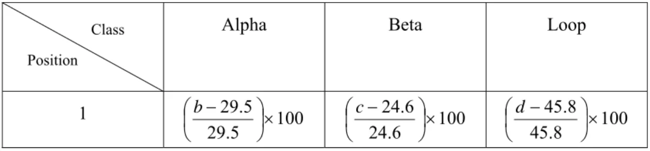
For example, assume that the proportion of the alpha, beta and loop structure among these 200 points for Position 1 are b%, c% and d %, respectively. Then we will check the change of distribution ratio corresponding to the original distribution ratio and this is shown as follows:
Table 3.1. The change of distribution ratio corresponding to the original ratio
Alpha Beta Loop
1 100 5 . 29 5 . 29 × ⎟ ⎠ ⎞ ⎜ ⎝ ⎛ −b 100 6 . 24 6 . 24 × ⎟ ⎠ ⎞ ⎜ ⎝ ⎛ −c 100 8 . 45 8 . 45 × ⎟ ⎠ ⎞ ⎜ ⎝ ⎛ −d Position Class
Under this condition, we can see the percentage change of the distribution ratio easily. The class label will be determined to be the maximum gain change of the ratio among these three types of secondary structure. In the same way, this process will be performed a times for each amino acid sequence.
3.4 Fusion Method
3.4.1 Majority Vote Based on the Global Confidence Value
Since we have proposed two different approaches based on the VDM table and the PSIPRED to predict the protein secondary structure, we certainly have a great interest in combining these three methods and eager to raise the overall accuracy after this fusion work. The first idea that we have hit upon is also the majority vote scheme. Every position of the input testing sequence will certainly have three predicted class labels using VDM table method with nearest neighbor majority vote, VDM table method with nearest neighbor balanced prediction and PSIPRED respectively. The ideal case is that these three different methods have the same ability to predict the α, ß and loop class. Then we can simply take a vote between these three predicted classes. Unfortunately, this thing will definitely not occur in the real life. Having this cognition, we make an overall prediction among the 120 proteins by using three different approaches first and then find out the individual accuracy for α, ß and loop class respectively. We regarded these as the global confidence value for three classes. After this work, when any testing sequence comes and has three class labels for any position, we will not take a vote between these three class labels to decide the class it
belongs to. Let us make an example to illustrate this approach.
Assume that the individual accuracy of the α, ß and loop classes with three different approaches are show below:
Table 3.2. The individual accuracy of three classes with three different approaches VDM_NN_MV VDM_NN_BP PSIPRED Alpha a % b % c % Beta d % e % f % Loop g % h % i % Class Method
Assume that a part of a testing sequence of length 3 is predicted by the three different methods and it is shown below:
Table 3.3. The class labels predicted by three different methods
VDM_NN_MV VDM_NN_BP PSIPRED
1 Alpha Alpha Beta
2 Beta Beta Alpha 3 Alpha Beta Loop
Position Method
If we only take a simple vote between these three class labels, position one and position two will be determined easily due to the majority win. But position three will be ambiguous. So we need to make another table to calculate the total global confidence values for α, ß and loop class respectively and it is shown below:
Table 3.4. The total global confidence value table for each position
Alpha Beta Loop
1 a % + b % f % 0
2 c % d % + e % 0
3 a % e % i %
Position Class
Under this condition, the final class label for each position will be determined by the largest number of each row in the table and the ambiguous condition can also be avoided at the same time. In chapter 4, we will see the difference between prediction ability for the three classes for different approaches.
3.4.2 Majority Vote Based on the Local Confidence Value
In the last section, we have tried to combine the three different methods based on the global confidence value concept. In order to get the global confidence value, we need to test the overall proteins in advance and it usually takes a long time. Then, how to combine the three different methods without doing this and can still obtain some significant information from each method is the new problem we have to face now. In opposition to the global confidence value, we have proposed the local confidence values to reveal the three class probability for each predicted position in real-time. PSIPRED is developed by the neural network. As a result, the reliance of three states is available from the program. For the VDM table with nearest neighbor majority vote method, the reliance for three states is the distribution ratio for each
class. Finally, for the VDM table with nearest neighbor balanced prediction method, the reliance for three states is the change of distribution ratio corresponding to the original ratio. Under this condition, each predicted position will have 9 local confidence values. Let us make an example to illustrate this approach.
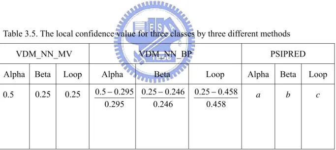
Assume that we make the 200 nearest neighbors for two VDM approaches and the original distribution ratio for α, ß and loop in our data set are 29.5%, 24.6% and 45.8%, respectively. Among these 200 neighbors, assume that 100 are labeled as α, 50 are labeled as ß and 50 are labeled as loop. The PSIPRED local confidence value for three states are a, b and c which are obtained from the neural network program. So the 9 local confidence values can be obtained and is shown as below:
Table 3.5. The local confidence value for three classes by three different methods
VDM_NN_MV VDM_NN_BP PSIPRED
Alpha Beta Loop Alpha Beta Loop Alpha Beta Loop
0.5 0.25 0.25 a b c 295 . 0 295 . 0 5 . 0 − 246 . 0 246 . 0 25 . 0 − 458 . 0 458 . 0 25 . 0 −
The next work we should do is to make a sum of each confidence value for each class. For alpha class, the total confidence value will be (0.5+0.695+a). The beta and the loop confidence value will be (0.25+0.016+b) and (0.25–0.454+c), respectively. Finally, the predicted class will be determined with the largest number in the sum.
Chapter 4. Experiment and Simulation Results
4.1 Introduction to Data Sets
The database of our research is a part of HSSP [19], [20] database and has less
than 25% sequence identity by using BLAST testing. There are totally 120 proteins in our database and it is shown in Table 4.1. HSSP (homology-derived structures of
proteins) is a derived database merging information from 3-D structure and 1-D
sequence of proteins. For each protein of known 3-D structure from the Protein Data Bank (PDB), the database has a multiple sequence alignment of all available homologues and a sequence profile characteristic of the family. The list of homologues is the result of a database search in SWISSPROT using a position-weighted dynamic programming method for sequence profile alignment. The database is updated frequently. The listed homologues are very likely to have the same 3-D structure as the PDB protein to which they have been aligned. The database is not only a database of aligned sequence families, but also a database of implied secondary and tertiary structures covering 29% of all SWISSPROT-stored sequences.
Table 4.1. The database of this research
1a45 1acx 1azu 1bbp 1bds 1bks 1bmv 1cbh 1cc5 1cdh
1cdt 1crn 1cse 1cyo 1dur 1eca 1etu 1fc2 1fdl 1fkf 1fnd 1fxi 1g6n 1gd1 1gdj 1gpl 1hip 1il8 1l58 1lap 1lmb 1mcp 1mrt 1ovo 1paz 1ppt 1prc 1pyp 1r09 1rbp 1rhd 1s01 1sh1 1tgs 1tnf 1ubq 2aat 2ak3 2alp 2cab 2ccy 2cyp 2fox 2fxb 2gbp 2gls 2gn5 2hmz 2i1b 2lhb
2ltn 2mev 2mhu 2or1 2pab 2pcy 2phh 2rsp 2sns 2sod
2stv 2tgp 2tmv 2tsc 2utg 2wrp 3ait 3blm 3cla 3cln 3ebx 3hmg 3icb 3pgm 3rnt 3sdh 3tim 4bp2 4cms 4cpa 4cpv 4gr1 4pfk 4rhv 4rxn 4sgb 4ts1 4xia 5cyt 5er2 5hvp 5ldh 5lyz 6acn 6cpa 6cpp 6cts 6dfr 6hir 6tmn 7cat 7icd 7rsa 8abp 8adh 9api 9ins 9pap 9wga 256b
Let us make a simple introduction to the content and format of the HSSP files. One HSSP file contains a structural protein family: one testing protein of known structure and all its structurally homologous relatives from the database of known sequences. The file is divided into four blocks: HEADERS, PROTEINS, ALIGNMENTS and SEQUENCE PROFILE. The HEADERS block is mandatory and the other three blocks are present only if at least one homologous alignment is found and each of the additional blocks begins with the string “##.” File organization is line-oriented. SEQLENGTH, NCHAIN and NALIGN which indicate the length of the sequence, the number of distinct chains and the number of aligned sequences, respectively. The PROTEINS block shows the pair alignment data for each of the
proteins deemed structurally homologous to the testing protein, where the word pair alignment refers to the alignment of the testing protein with the single homologous protein. The ALIGNMENTS block indicates the residue-by-residue details of the family alignment. Finally, the SEQUENCE PROFILE block shows the relative frequency for each of the 20 amino acid residue in a given sequence position, from counting the residue at that position in each of the aligned sequences including the testing sequence. A value of 100 means that at this position only one type of amino acid is found. As a result, we get the amino acid and corresponding secondary structure from the ALIGNMENTS block section for 120 different HSSP files and then our data sets are established. After building up our data sets, we can use two different VDM-based nearest neighbor methods, PSIPRED and two fusion methods to make the prediction. The experiment results are shown in the following sections.
4.2 Simulation Results of VDM Method with Nearest Neighbor Majority Vote
Since we use the nearest neighbor scheme to make the prediction, we choose the 100, 150 and 200 nearest neighbors to run the simulation in this research. The simulation results of VDM method with nearest neighbor majority vote for different number of nearest neighbors are shown as follows:
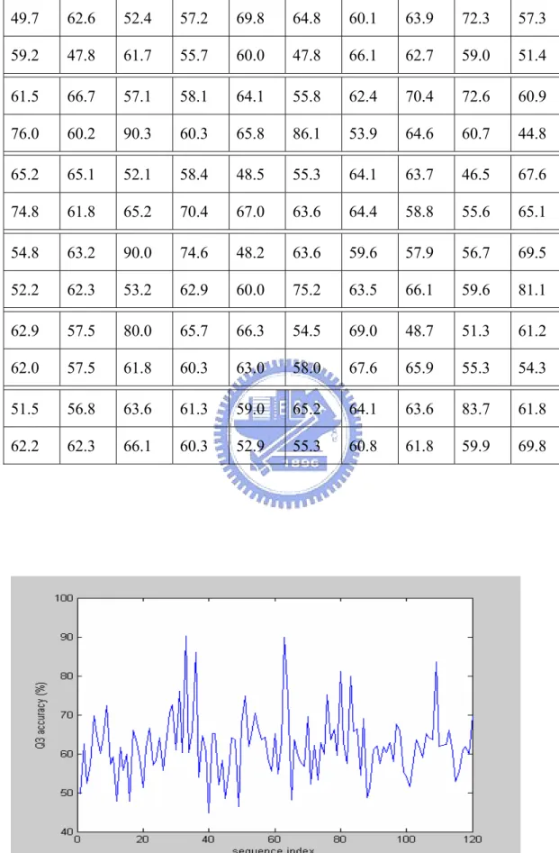
Table 4.2 The accuracy of 120 proteins with VDM_100-NN_MV method (%) 49.7 62.6 52.4 57.2 69.8 64.8 60.1 63.9 72.3 57.3 59.2 47.8 61.7 55.7 60.0 47.8 66.1 62.7 59.0 51.4 61.5 66.7 57.1 58.1 64.1 55.8 62.4 70.4 72.6 60.9 76.0 60.2 90.3 60.3 65.8 86.1 53.9 64.6 60.7 44.8 65.2 65.1 52.1 58.4 48.5 55.3 64.1 63.7 46.5 67.6 74.8 61.8 65.2 70.4 67.0 63.6 64.4 58.8 55.6 65.1 54.8 63.2 90.0 74.6 48.2 63.6 59.6 57.9 56.7 69.5 52.2 62.3 53.2 62.9 60.0 75.2 63.5 66.1 59.6 81.1 62.9 57.5 80.0 65.7 66.3 54.5 69.0 48.7 51.3 61.2 62.0 57.5 61.8 60.3 63.0 58.0 67.6 65.9 55.3 54.3 51.5 56.8 63.6 61.3 59.0 65.2 64.1 63.6 83.7 61.8 62.2 62.3 66.1 60.3 52.9 55.3 60.8 61.8 59.9 69.8
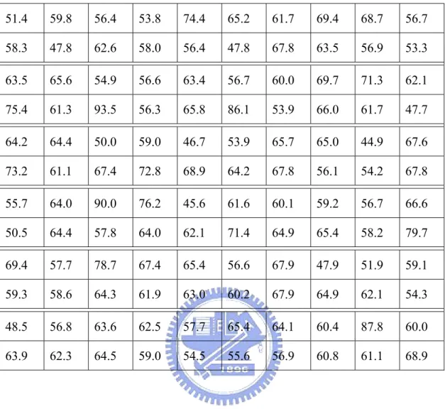
Table 4.3 The accuracy of 120 proteins with VDM_150-NN_MV method (%) 51.4 59.8 56.4 53.8 74.4 65.2 61.7 69.4 68.7 56.7 58.3 47.8 62.6 58.0 56.4 47.8 67.8 63.5 56.9 53.3 63.5 65.6 54.9 56.6 63.4 56.7 60.0 69.7 71.3 62.1 75.4 61.3 93.5 56.3 65.8 86.1 53.9 66.0 61.7 47.7 64.2 64.4 50.0 59.0 46.7 53.9 65.7 65.0 44.9 67.6 73.2 61.1 67.4 72.8 68.9 64.2 67.8 56.1 54.2 67.8 55.7 64.0 90.0 76.2 45.6 61.6 60.1 59.2 56.7 66.6 50.5 64.4 57.8 64.0 62.1 71.4 64.9 65.4 58.2 79.7 69.4 57.7 78.7 67.4 65.4 56.6 67.9 47.9 51.9 59.1 59.3 58.6 64.3 61.9 63.0 60.2 67.9 64.9 62.1 54.3 48.5 56.8 63.6 62.5 57.7 65.4 64.1 60.4 87.8 60.0 63.9 62.3 64.5 59.0 54.5 55.6 56.9 60.8 61.1 68.9
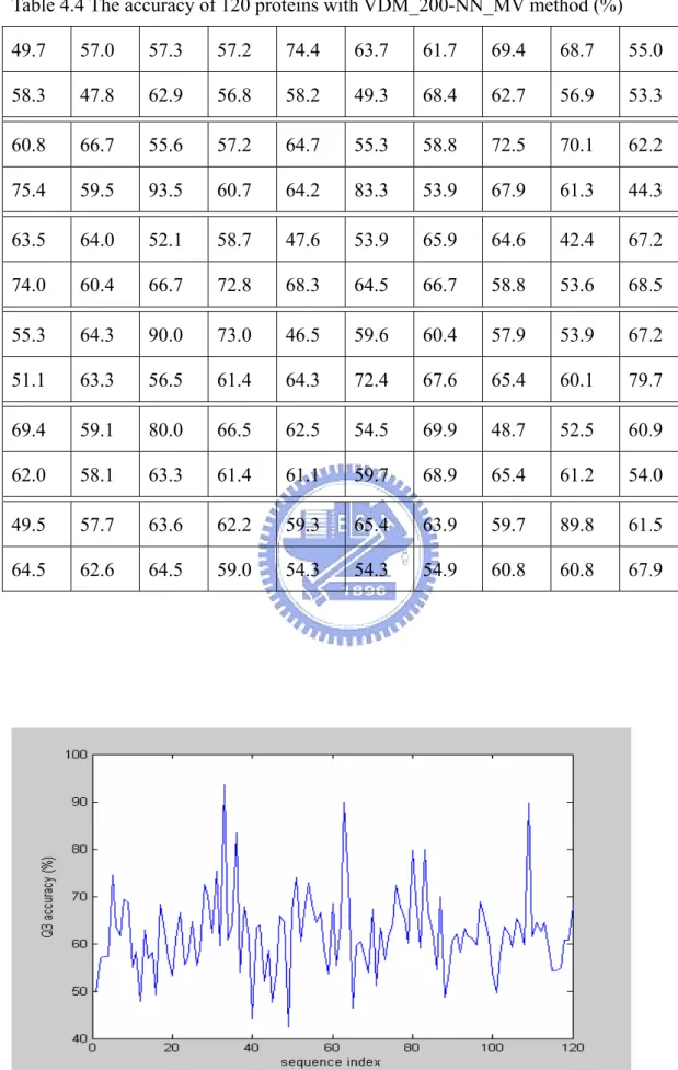
Table 4.4 The accuracy of 120 proteins with VDM_200-NN_MV method (%) 49.7 57.0 57.3 57.2 74.4 63.7 61.7 69.4 68.7 55.0 58.3 47.8 62.9 56.8 58.2 49.3 68.4 62.7 56.9 53.3 60.8 66.7 55.6 57.2 64.7 55.3 58.8 72.5 70.1 62.2 75.4 59.5 93.5 60.7 64.2 83.3 53.9 67.9 61.3 44.3 63.5 64.0 52.1 58.7 47.6 53.9 65.9 64.6 42.4 67.2 74.0 60.4 66.7 72.8 68.3 64.5 66.7 58.8 53.6 68.5 55.3 64.3 90.0 73.0 46.5 59.6 60.4 57.9 53.9 67.2 51.1 63.3 56.5 61.4 64.3 72.4 67.6 65.4 60.1 79.7 69.4 59.1 80.0 66.5 62.5 54.5 69.9 48.7 52.5 60.9 62.0 58.1 63.3 61.4 61.1 59.7 68.9 65.4 61.2 54.0 49.5 57.7 63.6 62.2 59.3 65.4 63.9 59.7 89.8 61.5 64.5 62.6 64.5 59.0 54.3 54.3 54.9 60.8 60.8 67.9
Let us make a summary for this method. The overall average accuracy of the 120 proteins for 100, 150 and 200 nearest neighbors are 60.8%, 61.0% and 61.5% respectively. The standard deviations are 8.27, 8.56 and 8.62, respectively. Furthermore, the average accuracies for alpha, beta and loop classes are shown below. These will be very significant when we make a fusion work with PSIPRED in the later section.
Table 4.5 The average accuracies and standard deviations of 120 proteins
Method Average Accuracy Standard Deviation
VDM_100-NN_MV 60.8% 8.27
VDM_150-NN_MV 61.0% 8.56
VDM_200-NN_MV 61.5% 8.62
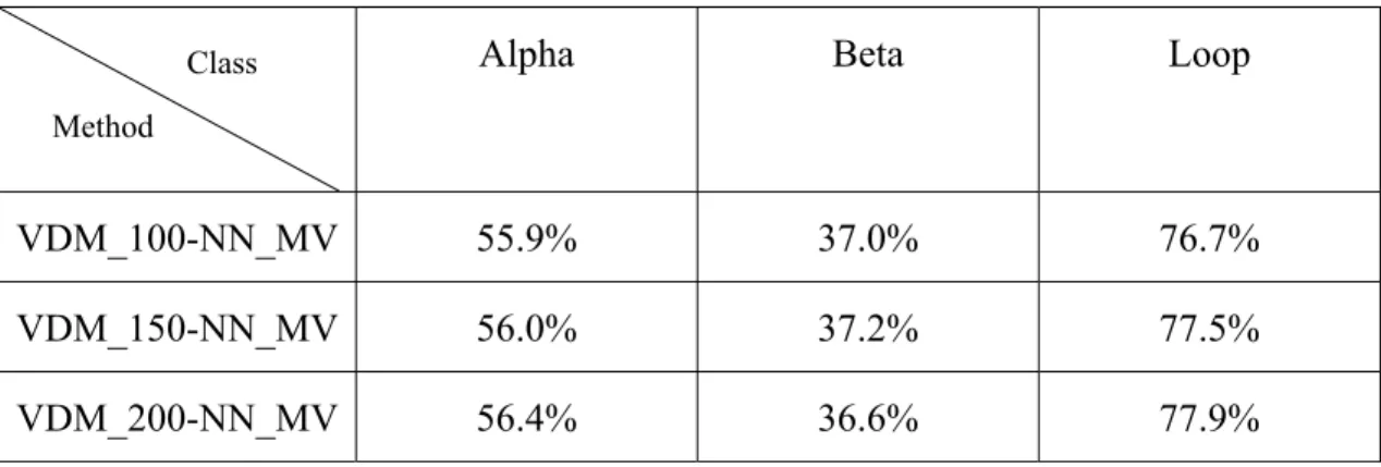
Table 4.6 The average accuracies for three classes with different No. of neighbors
Alpha Beta Loop
VDM_100-NN_MV 55.9% 37.0% 76.7%
VDM_150-NN_MV 56.0% 37.2% 77.5%
VDM_200-NN_MV 56.4% 36.6% 77.9%
Method Class
4.3 Simulation Results of VDM Method with Nearest Neighbor Balanced Prediction
Based on the nearest neighbor method, we also choose the nearest 100, 150 and 200 nearest neighbors to run the simulation in this research. The simulation results of VDM method with nearest neighbor balanced prediction for different number of nearest neighbors are shown as follows:
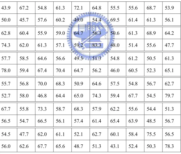
Table 4.7 The accuracy of 120 proteins with VDM_100-NN_BP method (%)
43.9 67.2 54.8 61.3 72.1 64.8 55.5 55.6 68.7 53.9 50.0 45.7 57.6 60.2 49.0 54.4 69.5 61.4 61.3 56.1 62.8 60.4 55.9 59.0 64.7 56.3 50.6 61.3 68.9 64.2 74.3 62.0 61.3 57.1 59.2 83.3 48.0 51.4 55.6 47.7 57.7 58.5 64.6 56.6 49.3 51.3 54.8 61.2 50.5 61.3 78.0 59.4 67.4 70.4 64.7 56.2 46.0 60.5 52.3 65.1 55.7 56.8 70.0 68.3 50.9 64.6 57.5 54.8 56.7 62.7 52.7 58.0 46.8 64.4 65.0 74.3 59.4 67.7 54.5 79.7 67.7 55.8 73.3 58.7 68.3 57.9 62.2 55.6 54.4 51.3 56.5 54.7 66.5 56.1 57.4 61.4 65.4 63.9 48.5 56.7 54.5 47.7 62.0 61.1 52.1 62.7 60.1 58.4 75.5 56.5 56.0 62.6 67.7 65.6 48.7 51.3 43.1 52.4 50.3 78.3
Table 4.8 The accuracy of 120 proteins with VDM_150-NN_BP method (%) 44.5 66.4 56.5 63.6 72.1 65.4 57.4 52.8 66.3 57.3 51.7 45.7 59.3 61.4 47.3 53.7 67.8 62.2 61.9 57.0 63.9 59.4 55.4 58.4 64.7 55.1 48.2 65.5 70.7 63.6 73.2 62.7 61.3 59.4 60.8 77.8 47.0 51.1 55.0 51.1 56.7 58.9 54.2 56.6 52.4 53.9 56.1 62.8 51.0 60.2 79.5 58.4 65.2 74.1 67.3 56.4 43.7 65.8 51.6 65.8 52.6 57.7 63.3 73.0 49.1 65.7 58.1 57.5 51.0 62.7 53.8 58.4 47.4 63.3 62.9 73.3 59.5 67.3 56.8 81.8 66.1 57.5 76.0 57.0 66.3 57.9 64.7 51.3 54.1 51.0 56.5 55.3 65.2 54.7 59.3 63.6 66.0 61.8 48.5 57.3 55.6 47.1 60.5 61.0 51.1 61.7 60.1 57.8 77.6 58.0 56.2 62.6 71.8 66.2 50.5 51.9 43.1 55.2 52.9 77.4
Table 4.9 The accuracy of 120 proteins with VDM_200-NN_BP method (%) 45.1 65.4 54.8 63.6 74.4 64.5 57.4 55.6 67.5 54.0 53.3 47.8 59.3 59.1 45.5 53.7 67.2 61.4 63.1 57.9 62.8 58.3 55.4 58.1 64.1 54.2 47.1 62.7 70.7 64.4 74.3 63.3 71.0 58.5 60.0 77.8 47.3 51.1 55.2 51.1 56.7 59.3 58.3 54.8 51.8 53.9 56.0 62.8 51.0 62.5 77.2 58.0 68.1 74.1 66.3 56.7 43.7 64.0 51.0 67.8 55.3 57.6 56.7 69.8 47.4 62.6 57.5 57.5 54.6 63.6 53.8 58.7 48.0 63.6 67.9 71.4 56.8 66.9 58.2 80.4 69.3 57.7 77.3 56.1 69.2 58.6 65.1 52.1 54.1 52.5 57.4 57.3 66.8 55.2 57.4 64.0 64.8 62.3 47.6 56.1 56.6 46.2 62.0 61.4 53.4 60.5 59.2 58.4 79.6 59.0 57.2 63.0 68.5 66.2 49.2 52.4 43.1 57.5 53.2 76.4
Let us make another summary for this balanced prediction method. The average accuracy of the 120 proteins for 100, 150 and 200 nearest neighbors are 58.1%, 59.4% and 59.7%, respectively. The standard deviations are 7.89, 7.97 and 7.98, respectively. Furthermore, the average accuracies for alpha, beta and loop classes are shown below. These will also be very significant when we make a fusion work with PSIPRED in the later section.
Table 4.10 The average accuracies and standard deviations of 120 proteins
Method Average Accuracy Standard Deviation
VDM_100-NN_BP 58.1% 7.79
VDM_150-NN_BP 59.4% 7.97
VDM_200-NN_BP 59.7% 7.98
Table 4.11 The average accuracies for three classes with different No. of neighbors
Alpha Beta Loop
VDM_100-NN_BP 63.3% 56.8% 55.4%
VDM_150-NN_BP 63.6% 57.0% 56.2%
VDM_200-NN_BP 63.8% 57.4% 56.3%
Method Class
4.4 Simulation Results of PSIPRED
Table 4.12 The accuracy of 120 proteins with PSIPRED (%)
52.0 67.3 63.7 55.5 83.7 71.9 65.3 66.7 73.5 69.7 61.7 43.5 59.9 59.1 69.0 79.4 80.2 70.7 69.5 75.7 74.7 75.0 70.1 62.3 64.0 64.1 54.1 67.6 78.0 70.5 78.2 78.0 100 63.8 80.8 94.4 62.5 64.6 65.5 60.3 62.1 62.5 50.0 60.5 72.4 69.4 68.8 69.2 70.7 84.3 70.3 76.8 75.3 79.0 69.8 57.5 69.3 71.9 83.9 64.5 63.9 83.3 85.7 62.3 81.8 68.3 67.1 66.0 71.4 60.9 71.2 65.6 64.4 82.9 82.9 70.3 68.5 65.7 86.0 62.9 51.2 88.0 64.8 59.6 81.4 69.1 53.0 66.9 67.5 81.5 59.9 75.5 65.4 63.0 67.4 71.7 71.8 67.0 57.9 57.6 60.7 60.5 67.4 69.4 70.6 73.4 61.0 81.6 65.6 65.9 69.1 67.7 71.8 62.6 59.6 54.9 61.3 63.7 90.6 67.2
Fig. 4.7. The accuracy plot of 120 proteins with PSIPRED method.
The average accuracy of the 120 proteins for PSIPRED is 67.0% and the standard deviation is 9.4. The average accuracy for alpha, beta and loop class are shown below and these also will be useful when we make a fusion work.
Table 4.13 The average accuracy and standard deviation of 120 proteins
Method Average Accuracy Standard Deviation
PSIPRED 67.0% 9.4
Table 4.14 The average accuracy of PSIPRED for three classes
Alpha Beta Loop
PSIPRED 70.7% 58.7% 69.1%
Method Class
4.5 Simulation Results of Fusion Method
4.5.1 Results of Majority Vote Based on the Global Confidence Value
We make a fusion work in combining the VDM_NN_MV with VDM_NN_BP and PSIPRED first. Here we will have three fusion works (Fusion 1 – Fusion 3). Fusion 1 work is to make the fusion combination of VDM_100-NN_MV, VDM_100-NN_BP and PSIPRED. Fusion 2 work is to make the fusion combination of VDM_150-NN_MV, VDM_150-NN_BP and PSIPRED. Fusion 3 work is to make the fusion combination of VDM_200-NN_MV, VDM_200-NN_BP and PSIPRED. According to Section 3.4.1, the total global confidence values for each predicted residue will be weighted summed to determine the class which has the maximum weighted class value. We show these global confidence values and the fusion results as follows.
(1) Fusion 1:
Table 4.15 The global confidence values of three classes for three methods (Fusion 1)
Alpha Beta Loop
VDM_100-NN_MV 55.9% 37.0% 76.7% VDM_100-NN_BP 63.3% 56.8% 55.4% PSIPRED 70.7% 58.7% 69.1% Method Class
Table 4.16 The accuracy of 120 proteins for Fusion 1 (%) 52.0 69.2 57.3 60.1 81.4 68.5 61.9 61.1 75.9 64.0 58.3 45.7 63.2 60.2 61.8 58.8 71.8 65.9 64.0 57.0 65.2 69.8 58.4 62.0 66.0 59.7 57.6 71.1 74.3 67.2 77.7 67.9 90.3 60.3 70.8 88.9 53.2 65.7 62.7 50.0 62.8 65.8 56.2 62.3 51.3 56.6 63.4 64.8 53.5 69.1 80.3 63.5 70.3 74.1 70.6 64.0 58.6 64.0 58.2 71.1 61.8 62.9 86.7 73.0 55.3 71.7 62.1 59.2 61.7 70.2 53.3 65.5 55.2 65.5 68.6 77.1 66.2 69.3 60.1 82.5 71.0 57.0 81.3 65.2 65.4 62.1 69.1 53.0 55.0 61.4 66.7 57.3 69.6 62.3 63.0 66.5 70.1 69.0 57.3 60.3 58.6 53.8 65.1 64.3 61.9 66.4 65.7 61.0 83.7 60.9 61.2 65.0 71.0 66.9 54.8 56.1 54.9 59.4 61.1 81.1
Table 4.17 The average accuracy and standard deviation of 120 proteins
Method Overall Average Accuracy Standard Deviation
Fusion 1 63.0% 8.2
(2) Fusion 2:
Table 4.18 The global confidence values of three classes for three methods (Fusion 2)
Alpha Beta Loop
VDM_150-NN_MV 56.0% 37.2% 77.5%
VDM_150-NN_BP 63.6% 57.0% 56.2%
PSIPRED 70.7% 58.7% 69.1%
Method Class
Table 4.19 The accuracy of 120 proteins for Fusion 2 (%) 52.6 67.3 57.3 61.9 81.4 68.8 63.9 66.7 72.3 64.0 58.3 45.7 65.0 62.5 58.2 61.8 71.2 67.1 63.6 59.8 66.9 70.8 56.9 60.8 64.7 59.3 55.3 70.4 72.6 67.8 76.5 68.3 93.5 57.1 70.8 83.3 53.0 64.3 62.8 51.1 62.5 65.5 54.2 62.6 52.4 57.9 64.4 65.5 55.6 68.8 79.5 62.8 69.6 76.5 71.8 64.5 59.8 65.8 56.9 74.5 61.4 64.1 86.7 79.4 53.5 73.7 61.4 63.2 58.9 69.4 57.0 66.5 57.8 66.3 67.1 76.2 64.9 68.9 61.0 81.1 74.2 57.5 78.7 65.7 65.4 63.4 71.0 50.4 55.9 60.3 63.9 58.4 69.3 62.8 64.8 68.6 70.1 67.9 61.2 59.7 54.5 53.5 64.3 65.4 60.3 65.9 64.6 59.7 85.7 61.2 63.7 65.0 71.8 67.9 57.0 57.2 56.9 61.3 61.1 80.2
Table 4.20 The average accuracy and standard deviation of 120 proteins
Method Average Accuracy Standard Deviation
Fusion 2 63.3% 8.2
(3) Fusion 3:
Table 4.21 The global confidence values of three classes for three methods (Fusion 3)
Alpha Beta Loop
VDM_200-NN_MV 56.4% 36.6% 77.9%
VDM_200-NN_BP 63.8% 57.4% 56.3%
PSIPRED 70.7% 58.7% 69.1%
Method Class
Table 4.22 The accuracy of 120 proteins for Fusion 3 (%) 49.7 65.4 60.0 61.9 81.4 67.9 63.9 66.7 73.5 60.7 60.8 45.7 65.6 59.0 61.8 63.2 71.2 66.7 64.0 60.7 65.2 71.9 58.1 62.3 65.4 59.3 54.1 71.8 74.4 68.4 78.2 69.2 93.5 60.3 69.2 83.3 53.5 63.9 62.4 50.0 63.1 65.1 54.2 62.6 53.7 59.2 63.9 65.2 53.5 68.4 79.5 62.1 71.7 76.5 71.5 64.0 60.0 64.0 55.6 74.5 62.3 64.1 86.7 74.6 51.8 71.7 61.1 61.4 58.2 70.2 56.0 66.2 57.1 64.0 70.0 75.2 67.6 69.7 63.4 81.1 74.2 58.5 81.3 65.7 65.4 61.4 71.9 51.3 56.3 62.0 66.7 58.8 69.9 62.6 63.0 69.0 70.4 69.2 61.2 59.4 57.6 54.4 64.3 65.8 62.2 65.2 64.8 59.0 87.8 62.5 64.7 65.7 70.2 67.5 54.8 55.9 56.9 61.8 61.1 80.2
Table 4.23 The average accuracy and standard deviation of 120 proteins
Method Average Accuracy Standard Deviation
Fusion 3 63.5% 8.2
4.5.2 Results of Majority Vote Based on the Local Confidence Value
In this section, we make a fusion work in combining the VDM_NN_MV with VDM_NN_BP and PSIPRED using the local confidence values of these three methods. We will propose three fusion works, Fusion 4 – Fusion 6. Fusion 4 work is the combination of the VDM_100-NN_MV, VDM_100-NN_BP and PSIPSED. Fusion 5 work is the combination of VDM_150-NN_NV, VDM_150-NN_BP and PSIPRED. Fusion 6 work is the combination of VDM_200-NN_BP, VDM_200-NN_MV and PSIPRED. The local confidence value of VDM_NN_MV scheme for each predicted position is the distribution ratio of the three classes. On the other hand, the local confidence value of VDM_NN_BP for each predicted position is the change of the distribution ratio corresponding to the original ratio of the database. Since PSIPRED is developed by neural network, the confidence value for each predicted residue can be obtained directly from the execution program. According to Section 3.4.2, the total local confidence values for each predicted residue will be weighted summed to determine the class which has the maximum weighted class value. The simulation results of Fusion 4 – Fusion 6 are shown as follows.
(1) Fusion 4: (VDM_100-NN_MV + VDM_100-NN_BP +PSIPRED)
Table 4.24 The accuracy of 120 proteins for Fusion 4 (%)
48.6 71.0 58.9 57.8 74.4 70.5 59.8 61.1 81.9 65.7 56.7 45.7 63.8 60.2 58.2 73.5 78.5 67.9 68.3 59.8 65.5 68.8 57.9 60.8 67.3 62.7 54.1 69.7 76.8 68.2 82.1 69.5 83.9 63.8 74.2 94.4 57.0 62.1 61.6 51.1 61.4 65.1 54.2 64.8 55.0 64.5 63.4 65.7 60.6 66.8 81.9 64.1 69.6 75.3 73.5 62.7 55.2 65.8 60.1 78.5 61.8 61.3 83.3 79.4 54.4 72.7 64.5 61.0 60.3 68.5 59.2 70.1 59.7 64.8 76.4 77.1 63.5 70.4 62.4 88.8 74.2 56.2 86.7 65.7 68.3 73.1 71.5 55.6 55.9 60.3 67.6 58.1 70.5 62.2 63.0 66.9 69.5 67.7 59.3 61.2 57.6 53.5 68.2 66.2 60.3 68.6 66.2 59.7 83.7 63.4 63.3 67.6 71.8 69.2 55.6 56.9 52.9 58.5 59.4 85.8
Table 4.25 The average accuracy and standard deviation of 120 proteins
Method Average Accuracy Standard Deviation
Fusion 4 64.0% 8.8
(2) Fusion 5: (VDM_150-NN_MV + VDM_150-NN_BP +PSIPRED)
Table 4.26 The accuracy of 120 proteins for Fusion 5 (%)
49.7 71.0 58.9 62.4 76.7 70.3 61.4 61.1 83.1 66.3 60.8 47.8 63.2 59.0 60.0 76.5 76.8 67.1 68.1 59.8 64.9 70.8 57.4 61.4 68.6 62.0 49.4 68.3 78.7 68.0 83.2 70.8 90.3 62.1 73.3 91.7 57.3 61.8 61.6 53.4 61.8 64.7 52.1 63.0 57.5 60.5 64.4 65.2 60.6 67.6 81.9 63.8 71.7 76.5 72.8 65.2 58.6 69.3 58.2 78.5 61.0 62.2 83.3 81.0 50.9 73.7 64.2 64.5 58.9 70.4 58.7 68.7 59.7 66.3 80.0 77.1 64.9 71.6 64.3 88.8 75.8 57.7 82.7 66.1 68.3 73.1 72.7 53.8 55.3 61.4 69.4 58.3 70.8 61.8 63.0 68.2 69.8 67.7 54.4 60.9 60.6 52.9 65.9 66.7 61.9 67.4 67.1 59.7 81.6 65.9 64.9 67.9 73.4 70.2 55.6 58.0 49.0 55.7 58.8 82.1
Table 4.27 The average accuracy and standard deviation of 120 proteins
Method Average Accuracy Standard Deviation
(3) Fusion 6: (VDM_200-NN_MV + VDM_200-NN_BP +PSIPRED)
Table 4.28 The accuracy of 120 proteins for Fusion 6 (%)
50.3 72.9 56.5 63.0 79.1 71.7 61.4 61.1 81.9 62.9 60.0 47.8 63.8 59.1 60.0 74.3 76.8 68.7 68.4 59.8 66.6 68.8 58.1 60.5 64.7 61.1 52.9 66.9 78.7 68.6 82.1 70.8 90.3 61.6 74.2 94.4 57.5 62.9 61.6 55.2 62.5 64.7 50.0 62.6 57.2 63.2 62.9 65.9 60.1 69.1 82.7 65.2 73.2 76.5 73.8 65.5 57.5 71.9 58.2 76.5 62.7 61.7 86.7 81.0 52.6 72.7 64.5 64.0 58.2 70.7 59.2 68.0 59.0 66.7 78.6 78.1 62.6 69.7 66.2 88.1 77.4 57.7 81.3 64.8 67.3 72.4 72.7 53.8 55.9 62.3 69.4 58.8 73.0 61.8 63.0 67.8 70.8 69.0 56.3 59.7 58.6 54.4 66.7 66.2 63.2 66.9 68.1 60.4 81.6 64.4 64.7 68.6 72.6 69.5 55.9 58.0 49.0 55.7 57.6 81.1
Table 4.29 The average accuracy and standard deviation of 120 proteins
Method Average Accuracy Standard Deviation