A MODIFIED H
2FEEDFORWARD ACTIVE
CONTROL SYSTEM FOR SUPPRESSING
BROADBAND RANDOM AND TRANSIENT NOISES
M. B H. CDepartment of Mechanical Engineering, Chiao-Tung University, 1001 Ta-Hsueh Road, Hsin-Chu 30050 Taiwan, Republic of China
(Received 2 November 1995, and in final form 16 April 1996)
Three feedforward active noise control algorithms based on H2, Ha, and modified H2 optimal model matching principles are investigated in this study. The first two methods provide significant attenuation for broadband random noises. However, the H2and Ha methods generally result in high-gain controllers at high frequencies, which calls for some truncation measures in the frequency domain. The third method effectively eliminates the high-gain problem of the ordinary H2 and Ha algorithms. In addition, this method is guaranteed to result in a causal and stable controller which is crucial in practical implementation. The algorithms are coded into controllers by using a floating-point digital signal processor. The experimental results show significant attenuation for stationary broadband random noises as well as transient impact noises in a duct.
7 1996 Academic Press Limited
1. INTRODUCTION
Active noise control (ANC) techniques serve as a useful alternative to conventional passive control methods because it provides numerous advantages such as improved low-frequency performance, reduction of size and weight, zero back pressure, reduction of energy consumption, and programmable flexibility of design [1]. A vast amount of literature has been produced in the last decade and a very good review can be found in Reference [2]. In the ANC configurations up to date, feedforward control has become the most widely used one (whenever the upstream reference signal is available) because it generally provides better performance in suppressing broadband noises within a moderate controller gain than the feedback control [2].
In this study, three feedforward active noise control algorithms based on H2, Ha, and
modified H2optimal model matching principles are investigated. These methods effectively
overcome the problem of the unstable inverse plant resulting from the inherent non-minimum phase (NMP) property of the cancellation path. The NMP behavior is a fundamental issue which is at the heart of the control system design, but often an overlooked factor that could seriously degrade the ANC performance in attenuating broadband random noises. Despite the effectiveness, the H2 and Ha methods generally
result in high-gain controllers at high frequencies, which calls for some truncation measures in the frequency domain during the controller design stage. To ease the problem, a modified H2 method has been developed to reduce the controller gain of the ordinary
H2and Ha algorithms. In addition, this method is guaranteed to result in a causal and
stable controller which is crucial in practical implementation. The feedforward algorithms are coded into ANC controllers by using a floating-point digital signal processor (DSP).
81
P(z)
C(z) S(z)
+
+
x(k) y(k)
The experimental results show significant attenuation for stationary broadband random noises in a duct. The proposed methods also have potential in suppressing transient impact noises that have been the major difficulty to adaptive methods.
Experiments are performed on a duct of finite length to justify the proposed methods. The experimental results obtained by using the H2and Hafeedforward techniques show
comparable attenuation for stationary noises as the popular filtered-x least mean square (LMS) method [3, 4]. The proposed methods also have potential in suppressing transient noises, e.g., the impact of a forge hammer.
This paper is organized as follows. First, the ANC algorithms based on H2 and Ha
optimization criteria will be briefly described. Then, a modified H2 method will be
developed for alleviating the high-gain problem associated with the ordinary H2and Ha
methods. In the following sections, the techniques developed will be validated by experimental investigations and the methods compared. In the final section, a conclusion of this work will be given.
2. THE ORDINARY H2AND Ha FEEDFORWARD ANC ALGORITHMS
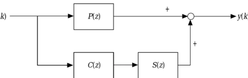
In the sequel, the formulations are expressed in terms of sampled-data systems and discrete-time base to facilitate the presentation and the digital implementation of the ANC algorithms. Consider the feedforward ANC problem of a finite-length duct, as shown in Figure 1. The sampled signal x(k) is the input disturbance noise. P(z) is the transfer function of the primary acoustic plant, where z denotes the z-transform variable. S(z) is the transfer function of the cancellation path composed of the actuator, the acoustic error path, and the sensor. This problem can be posed into a model matching problem, where the ANC problem amounts to finding the controller C(z) such that the residual field y(k) can be minimized. In order to match the characteristics of the paths P(z), C(z) and S(z), one is tempted to set
C(z) = −P(z)/S(z). (1)
However, it frequently occurs that S(z) is NMP, where direct application of equation (1) leads to a non-causal or unstable controller which is not implementable. It is then highly desirable to develop an ANC method that would effectively match the primary path and the cancellation path with respect to some optimal criteria when the NMP behavior is an issue. In this paper, two model matching algorithms capable of dealing with NMP problems in ANC applications are described.
The first approach is based on the H2 optimal criterion. Since the feedforward ANC
problem is equivalent to matching the characteristics of the primary path and the cancellation path, the degree of match can be measured using various criteria. The criterion
Figure 1. System block diagram of the feedforward ANC problem. P(z), S(z), and C(z) are the discrete-time transfer functions of the primary acoustic path, the secondary path, and the controller, respectively.
2 83
employed in the following method is the 2-norm in the Hilbert space. The squared error o2
2 is defined as follows:
o2
2=>P(z) + C(z)S(z)>22, (2)
where the 2-norm of a scalar transfer function is defined as
>G(z)>, 2
0
1 2pg
p −p =G(eju)=2du1
1/2 (3)The feedforward model matching problem then reduces to finding a biproper and stable transfer function (z) to minimize o2
2. The following derivation entails the so-called
inner-outer factorization. It can be shown that every proper and stable function T(z) has a factorization [5]
T(z) = Ta(z)Tm(z) (4)
with Ta(z) being an all-pass function and Tm(z) being a biproper minimum phase function. By assuming that the transfer function S(z) has been factored accordingly as
S(z) = Va(z)Vm(z) and substituting the factored form into equation (2) and omiting (z) for simplicity one obtains
o2
2=>P + VaVmC>22=>VaV−1a P+ VaVmC>22=>Va(V−1a P+ VmC)>22=>V−1a P+ VmC>22
(5) In the last step, Vahas a bounded constant magnitude on the unit circle. In Hilbert space,
V−1
a P can be uniquely decomposed into a stable part and an unstable part (by partial fraction expansion)
V−1
a P= (V−1a P)++ (V−1a P)−, (6)
where (V−1
a P)+, and (V−1a P)− correspond to the unstable part and the stable part
respectively. Note as these two terms belong to the subspaces that are orthogonal complements to each other. Then equation (5) can be developed into
o2
2=>(V−1a P)++ (V−1a P)−+ VmC>22=>(V−1a P)+>22+>(Va−1P)−+ VmC>22 (7)
The Pythagoras theorem in Hilbert space was used in the last equality. It is now clear that the unique optimal Copt (z) is
Copt(z) = −V−1m (V−1a P)s (8) and the minimum of o2
2 equals >(V−1a P)u>22. Note that this minimum value dictates the
ultimately achievable performance imposed by the NMP constraint.
Another elegant approach to match the characteristics of the primary path and the cancellation path is based on the Haoptimal criterion. Thea-norm of a scalar transfer
function G(z) is defined as
>G(z)>a= sup u$(−p,p)=G(e
ju)=, (9)
where sup denotes the least upper bound. As with the H2-norm optimization, the
feedforward ANC problem can be recast into that of finding a biproper and stable transfer function C(z) to minimize the a-norm error
The problem can now be formulated in terms of the a-norm as
min>P + SC>a= min>P + VaVmC>a= min>VaV−1a P+ VaVmC>a
= min>Va(V−1a P+ VmC)>a= min>V−1a P+ VmC>a (11)
where the inner-outer expansion of the transfer function S(z) and the property of the all-pass function =Va(eju)= = 1, u $(−p, p] have been used.
Next, define R = V−1
a Pand Q = −VmC. The problem in equation (13) is then reduced to finding a stable and proper Q(z) for a given proper (not necessarily stable) R(z) such that>R − Q>a is minimized. This is the well-known Nahari problem and the minimum
value can be shown to be the Hankel norm of the operator R [6].
A state space method is employed in this paper for solving the Nahari problem [6]. To keep the presentation to a reasonable length, the procedure of finding the optimal transfer functions Q(z) and C(z) is summarized as follows. In this algorithm packed matrix notation is used to denote the state-space realization, i.e., x(k + 1) = Ax(k) + Bu(k),
y(k) = Cx(k) + Du(k) is denoted as [A, B, C, D].
(1) Find the inner-outer factorization of the cancellation path: S(z) = Va(z)Vm(z) with both Vm(z) and V−1m (z) being proper and stable. (2) Find a minimal realization of R(z) and separate it into the stable part and the unstable part R(z) = [A, B, C, 0] + (stable part). (3) Solve the discrete-time Lyapunov equations for the controllability grammian Lcand the observability grammian Lo. Lc− ALcAT= BBT; Lo− ATLoA= CTC. (4) Find the maximum eigenvalue l2 of L
cLo and a corresponding eigenvector w. (5) Define
f(z) = [A, w, C, 0]; g(z) = [−AT,l−1, L
ow, BT, 0]. (6) Set Qopt(z) = R(z) −lf(z)/g(z). (7) Calculate the optimal controller Copt(z) = −V−1m (z)Qopt(z).
It should be noted that, unlike the H2method, the Hamethod per se is to achieve model
matching in an optimal way subject to the worst-case input [5]. The optimization of the
Hamethod is carried out for the whole class of input with bounded energy. Thus, the Ha
method tends to be more conservative than the H2 method in terms of performance.
3. THE MODIFIED H2FEEDFORWARD ANC ALGORITHM
As presented earlier, the H2 and Ha methods effectively solve the model matching
problem, even if the NMP problem of the plant is present. However, this masks somewhat a pitfall of the above methods. More precisely, excessive compensation for the NMP zeros by using the H2and Ha methods will generally result in unnecessary high gains at high
frequencies. The fact that the NMP zeros cluster at high frequencies is common for physical systems with flexibility [7], but other than that, it is more often than not the consequence of discretization of analog plants [8]. Compensation for these artificially generated NMP zeros is sometimes not worth the effort because the uncertainty of the NMP zeros obtained by experimental system identification methods is generally large at the plant zeros, where the plant output is extremely small. The NMP zeros impose inherent design constraints on the controller, wherein high-gains at high frequencies become inevitable. In practical implementation of the ANC controller, the effect of high-gains at high frequencies is very detrimental since they will saturate the actuator and one should avoid them whenever possible.
To alleviate the problem caused by the NMP zeros at high frequencies, remedies must be sought for designing the controller by using the H2and Haprinciples. Unfortunately,
a standard procedure of rolling-off by a low-pass filter stated in robust control literature [5, 9] would not seem to work for the present extremely high-order acoustic system (usually above 50). This is because the low-pass filter not only attenuates the high-frequency
2 85
magnitude but also introduces considerable phase shift that destroys the optimality of the controller. In practice, it is very difficult if not impossible to find a satisfactory compromise between the roll-off of magnitude and the invariance of phase, as manifested by Bode’s magnitude-phase relationship [10]. Hence, an alternative is employed in the present study to sample the frequency response function of the resulting controller and truncate the high-frequency portion. Then, the truncated frequency response function is inverse discrete Fourier transformed to yield the impulse response function which amounts to the coefficients of the finite impulse response (FIR) filter of the ANC controller. The reduced-gain controller can thus be safely used without saturating the actuator. Although the method should work for any stable system as it does in the present case, this heuristic approach is not based on any sort of optimality. In the sequel, a modified H2 algorithm
will be developed to eliminate the high-gain problem in a more elegant way.
In the proposed method, a key to elimating the high-gain problem is to introduce a constraint on the controller gain. This is done by modifying the 2-norm cost function in equation (2) into the following form:
J=>[P(z) + C(z)S(z)]>2
2+ r>C(z)> 2
2, (12)
where r is a weighting parameter which stipulates the relative importance of the control error and control effort. A large value of r corresponds to expensive control, while a small value corresponds to cheap control. Minimization of the cost function in equation (12) amounts to regulating the system response as close to the zero error of model matching while, on the other hand, keeping the gain of the controller as low as possible.
Using Parseval’s theorem in the z-domain, the cost function in equation (12) can be rewritten as
J=2pj1
G
=z= = 1
{[P(z) + C(z)S(z)][p(z−1) + C(z−1)S(z−1)] + rC(z)C(z−1)}z−1dz (13)
The stationary point of the cost function can be found by taking the first variation of J.
dJ =21pj
G
=z= = 1
{S(z)[P(z−1) + C(z−1)S(z−1)]dC(z) + S(z−1)[P(z) + C(z)S(z)]dC(z−1)
+ rC(z)dC(z−1) + rC(z)dC(z−1)}z−1dz = 0 (14)
Noting that, in the integrand, the terms associated withdC(z) and dC(z−1) are symmetrical
enables equation (14) to be simplified into
dJ =pj1
G
=z= = 1
[P(z)S(z−1) + C(z)S(z)S(z−1) + rC(z)]dC(z−1)z−1dz = 0 (15)
Before explicitly finding the solution of the optimal C(z), one first checks if the stationary point is a minimum by taking the second variation of J.
d2J=1
Let the plant S(z) be a proper and stable real rational function:
S(z) = N(z)/D(z). (17)
Then
S(z)S(z−1) + r = D*(z)D*(z−1)/D(z)D(z−1), (18)
where D*(z) is obtained from the following spectral factorization:
D*(z)D*(z−1) = N(z)N(z−1) + rD(z)D(z−1) (19)
with D*(z) and D*(z−1) containing all roots inside and outside respectively, the unit circle
=z= = 1. It is easy to verify that, if r $ 0, D*(z)D*(z−1) has no root on the unit circle, and
all roots are reciprocal. Thus, by substituting equation (18) into equation (16), the second variation of the cost function can be expressed
d2J=1 p
g
2p 0 =D*(eju)=2 =D(eju)=2 [dC(e ju)]2du (20)which is strictly positive and this confirms that the stationary point of the cost function is indeed the minimum.
Now one is in a position to solve equation (15) for the optimal controller. This can be accomplished by requiring the poles of the integrand to be strictly outside the unit circle. Let the integrand X(z) in equation (15) be expressed as
X(z) = C(z)F(z)F(z−1)z−1+ P(z)S(z−1)z−1, (21)
where
F(z) = D*(z)/D(z) (22)
whose poles are strictly inside the unit circle. For convenience, denote this by F(z)WC−,
where C−stands for the set of all real rational transfer functions with poles strictly inside
the unit circle. Set C+ may also be needed to indicate the complementary set of all real
rational transfer functions with poles on or strictly outside the unit circle. With some straighforward manipulations, equation (21) leads to
X(z)/F(z−1) − Q
+(z) = C(z)F(z)z−1+ Q−(z), (23)
where Q−(z)$C−and Q+(z)$C+are the stable and unstable part of P(z)S(z−1)z−1/F(z−1)
respectively. In equation (23), since all poles on the left hand side are outside the unit circle whilst all poles on the right hand side are inside the unit circle, the two sides are therefore independent and must both be equal to zero. From the right hand side of equation (23), one obtains the optimal solution of the controller Copt(z):
Copt(z) = −zQ−(z)/F(z) = ( − zD(z)/D*(z))[P(z)N(z−1)D(z−1)/zD(z−1)D*(z−1)−]
= (−zD(z)/D*(z))[P(z)N(z−1)/zD*(z−1)
−] (24)
where [·]−WC−denotes the stable part of a transfer function. If r$ 0, it is easy to verify
that the optimal controller in equation (24) is guaranteed to be causal and stable, which is crucial in on-line and real-time ANC implementations. It is also straighforward to show that the optimal controller will reduce to the ordinary H2 controller if r = 0 and to the
simple controller in equation (1) if, in addition, S(z) is the minimum phase. In summary, given the characteristics of the primary path and the secondary path, one may choose an
Antialiasing filter Power amp. Noise generator Closed if LMS Noise source PVC duct Loud speaker Noise 1.8 m 16 cm Microphone Antialiasing filter TMS320 Smoothing filter Power amp. 2 87
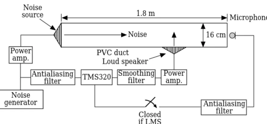
Figure 2. Experimental setup of the ANC system for a duct.
appropriate parameter r to calculate the modified H2 ANC feedforward controller
according to equation (24), provided that the spectral factorization in equation (19) has been obtained.
4. EXPERIMENTAL INVESTIGATIONS
Experiments were conducted to justify the developed modified H2 feedforward ANC
technique. Voltage signals are used as the reference inputs so that acoustic feedback can be ignored. The algorithms are implemented on a 32-bit floating-point digital signal processor TMS320C31 in conjunction with two-channel analog inputs and outputs. A circular PVC duct of length 1·8 m and diameter 16 cm was chosen for the test. The corresponding cutoff frequency of the duct is 1075 Hz. This renders the effective control bandwidth below approximately 1 kHz, where only plane waves are of interest. Two third order Bessel filters are used as the anti-aliasing filter and the smoothing filter, respectively. The ANC system, including the digital controller, the signal conditioning circuit, the sensor, and the actuator, is schematically shown in Figure 2. Four ANC algorithms are employed to suppress various synthetic noises and practical noises. The primary noises used in the experiments include the Guassian white noise, an engine noise, a blower noise, and an impact noise.
When implementing the digital controllers, the models of P(z) and S(z) must be determined prior to finding C(z). To this end, a parametric system identification procedure is utilized to establish a mathematical model of the transducer-duct system. First, the sampled input signal u(k) and the output signal y(k) are recorded by a data acquisition system. Then a parametric model is estimated on the basis of these input and output data. The white noise is selected as the input signal since it satisfies the condition of persistent
excitation, as required by a reliable system identification [12]. The parametric model adopted in this study is the autoregressive with exogenous input (ARX) model
y(k) = G(z)u(k) + H(z(e)k), k= 1, 2, . . . ,a, (25) where z is the shift operator, G(z) is the plant transfer function to be identified, and H(z) is the transfer function associated with the disturbance process. In ARX model, the transfer functions G(z) and H(z) take the following forms:
where N is the delay in samples, A(z−1) and B(z−1) are polynomials in z−1, i.e.,
A(z−1) = 1 + a
1z−1+ ··· + anaz−na, B(z−1) = b1+ b2z−1+ ··· + bnbz−nb + 1 (27) with the numbers na and nb − 1 being the orders of the respective polynomials. Hence, the model in equation (25) can be written as
A(z−1)y(k) = B(z−1)u(k − nk) + e(k). (28)
The system identification is essentially a time-domain curve-fitting procedure that estimates these (na + nb) parameters in the ARX model by, for example, the least square method. Details can be found in Reference [12].
For the transducer-duct systems, the aforementioned parametric identification procedure was employed to set up the corresponding mathematical models. First, the input data (white noise) and the output data were recorded by a signal analyzer, based on a sampling rate of 4 kHz. Second, the output data were shifted and interpolated to accommodate the additional delay due to the I/O operations of the DSP. Third, the
T 1
The mathematical models of the primary path and the cancellation path identified by the ARX procedure
P(z) S(z)
ZXXXXXCXXXXXV ZXXXXXCXXXXXV
delay = 22, gain = 0·0613 delay = 16, gain = 0·2724
ZXXXXXXXXCXXXXXXXXV ZXXXXXXXXCXXXXXXXXV
zeros poles zeros poles
*−7·7165 0·86852 0·4815i *−1·1551 −0·94322 0·0972i
*1·01252 0·0097i 0·89612 0·4144i *−1·04842 0·0776i −0·94572 0·2103i 0·92442 0·3464i 0·92352 0·3163i −0·95002 0·2785i −0·84122 0·2888i 0·79642 0·4002i 0·95052 0·1799i *−0·88522 0·4751i −0·82932 0·4289i 0·58812 0·7941i 0·97072 0·0639i −0·70362 0·5822i −0·81652 0·4748i 0·63422 0·5526i 0·79232 0·5989i *−0·65002 0·7641i −0·74892 0·6045i 0·46782 0·7088i 0·71552 0·6874i −0·50272 0·8538i −0·67222 0·7225i 0·25762 0·8202i 0·62212 0·7764i −0·25772 0·9553i −0·58892 0·7888i 0·02952 0·9770i 0·53652 0·8248i −0·34702 0·7281i −0·46872 0·8662i −0·10632 0·8638i 0·47442 0·8684i −0·08312 0·9795i −0·33082 0·9195i −0·29892 0·8328i 0·33612 0·9300i 0·11462 0·9880i −0·22142 0·9537i −0·56782 0·7791i 0·22012 0·9597i 0·29722 0·9535i −0·08512 0·9640i
−0·9672 0·08882 0·9885i 0·46372 0·8560i 0·00442 0·9789i
−0·89752 0·2670i −0·00722 0·9647i 0·63662 0·7678i 0·08792 0·9816i −0·80042 0·4315i −0·07372 0·9836i 0·76742 0·6358i 0·21642 0·9564i −0·67302 0·5743i −0·21912 0·9520i *1·01902 0·0087i 0·33352 0·9264i −0·39592 0·6569i −0·32562 0·9223i 0·94462 0·2904i 0·46282 0·8351i
−0·2394 −0·46232 0·8605i 0·87202 0·4686i 0·53822 0·8238i
−0·56292 0·8007i 0·52442 0·4154i 0·62142 0·7717i
−0·60322 0·7403i 0·71652 0·6872i −0·67572 0·6740i 0·79262 0·5979i −0·76652 0·5842i 0·86372 0·4759i −0·82542 0·4690i 0·89842 0·4143i −0·86502 0·3833i 0·93232 0·3004i −0·90412 0·2615i 0·95422 0·1953i −0·88342 0·2204i 0·98382 0·0588i −0·95702 0·0480i 0·98382 0·0588i −0·9518 −0·0493
20 0 –20 (a) –40 Magnitude (dB) 200 –200 100 0 –100 Phase (degree) 20 –40 0 –20 (b) Magnitude (dB) Frequency (Hz) 800 200 –200 0 Phase (degree) 500 100 0 –100 100 200 300 400 600 700 2 89
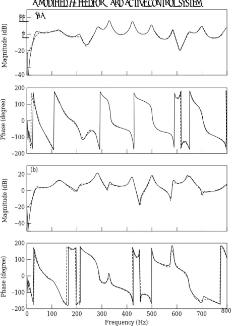
Figure 3. Comparison between the measured and the regenerated freqency response functions. (a) Frequency response function between the primary noise and the sensor: P(ejv); (b) frequency response function between the
canceling loudspeaker and the sensor: S(ejv). ——, Measured data; ----, regenerated data.
coefficients of the ARX model were estimated by choosing appropriate orders and the delay. This process might take several iterations until the magnitude and the phase of the measured and the regenerated frequency response functions were well matched and the ARX model orders were selected according to the Akaike’s information theoretical criterion (AIC) [12]. The poles and zeros of the transfer functions of the primary path and the cancellation path identified by using the ARX model are shown in Table 1 and their frequency response functions are shown in Figure 3. Note that there are 9 NMP zeros in the plant S(z). Comparison of the system delays between the two paths reveals that the causality was not violated, which is critical for feedforward ANC configurations. Excellent agreement was obtained between the measured and the regenerated frequency response
0 Magnitude (dB) 0 Frequency (Hz) 400 60 800 1200 1600 2000 40 20 0 –20 –40 –60
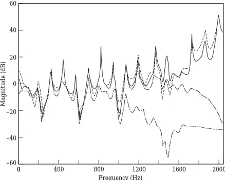
functions except for the frequency range below approximately 50 Hz, where the low-frequency responses of the loudspeakers were poor. Consequently, the control bandwidth was restricted to approximately 50–800 Hz. To show the effectiveness of the modified H2 formulation for reducing the high frequency gain, the magnitudes of the
controller frequency responses obtained from the H2 method, the Ha method, and the
modified H2methods (r = 0·01 and 1 respectively) are compared in Figure 4. The ordinary
H2and Hamethods led to high gains above approximately 1·2 kHz, which would saturate
the actuator. On the other hand, the modified H2 method indeed resulted in an optimal
controller with moderate gain at high frequencies and it could be implemented readily by using either an IIR filter or an FIR filter. Naturally, the cost of reducing the gain at high frequencies by choosing a large r value, e.g., r = 1 in the above case, was some degradation at the low frequencies. In the sequel, the results obtained from five ANC experiments will be presented.
In the first case, a Gaussian white noise was used as the primary noise. The H2method,
the Hamethod, the modified H2method, and the filtered-x LMS method were compared.
In this case, the ordinary H2and Hamethods were implemented by 768-tapped FIR filters
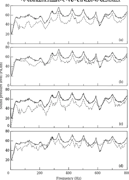
because of the high-gain problem. The procedure of frequency truncation has been given previously. In the filtered-x LMS method, the filter length was 256 and the step size was 0·01. The sound pressure spectra (20 averages) before and 2 min after ANC was activated are shown in Figure 5. The total noise attenuation in the band 50–800 Hz obtained by using the H2method, the Ha method, the modified H2 method, and the filtered-x LMS
method was found to be 9·3 dB, 7·3 dB, 9·5 dB, and 6·2 dB respectively. Among the methods, the H2 method and the modified H2 method appeared to provide the best
attenuation of the broadband random noise, especially at low frequencies (approximately 10–25 dB at 50–200 Hz).
Figure 4. The magnitudes of the controller frequency responses obtained from the feedforward ANC methods. ——, H2; – – – Ha; — - — modified H2(r=0·01); — — — modified H2(r = 1).
Sound pressure level (Pa,dB) 0 0 Frequency (Hz) 200 400 600 800 0 0 60 40 (a) 80 20 60 40 0 (b) 80 20 60 40 (c) 80 20 60 40 (c) 80 20 60 40 (d) 80 20 60 40 (d) 80 20 2 91
Figure 5. The sound pressure spectra for the Gaussian white noise before and after ANC was activated. (a)
H2method; (b) Hamethod; (c) modified H2method; (d) filtered-x LMS method. The step size used in filtered-x
LMS was 0·01, the filter length is 256, and the result was obtained 2 min after the algorithm was activated. ——, Before control; ----, after control.
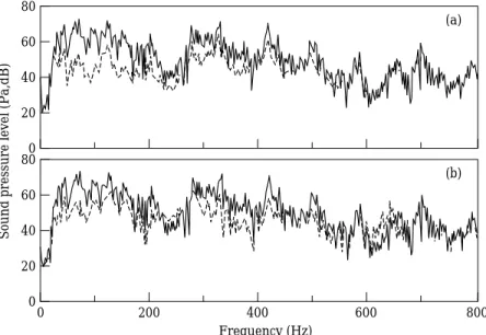
In the second case, an exhaust noise from the gasoline engine of a 2 l car operating at 4000 rpm was chosen as a more practical primary noise. To save space, only the results (20 averaged power spectra of sound pressure) obtained from the modified H2method and
the filtered-x LMS method are shown in Figure 6. The total noise attenuation obtained from the modified H2 method and filtered-x LMS method appeared to give more
attenuation at larger peaks (due to the problem of eigenvalue disparity [13]), while the modified H2 method yielded attenuation throughout the band.
In the third case, the noise from a blower with a radial fan operating at 3000 r.p.m was used as the primary noise. The noise contained harmonics associated with the blade-passing frequency and broadband components due to turbulence. The results (20 averaged per spectra of sound pressure) obtained from the modified H2method and the
100
0
Frequency (Hz) Sound pressure level (Pa,dB) 60
40 20 200 400 600 800 (b) 100 60 40 20 (a) 80 80 80 0 0 Frequency (Hz)
Sound pressure level (Pa,dB)
60 40 20 200 400 600 800 (b) 80 0 60 40 20 (a)
Figure 6. The sound pressure spectra for the engine noise of a car before and after ANC was activated. (a) Modified H2method; (b) filtered-x LMS method. The step size used in the filtered-x LMS was 0·005, the filter
length was 256, and the result was obtained 2 min after the algorithms was activated. ——, Before control; ----, after control.
filtered-x LMS method is shown in Figure 7. The total noise attenuation of the modified
H2method and the filtered-x LMS method was found to be 9·9 dB and 8·3 dB respectively.
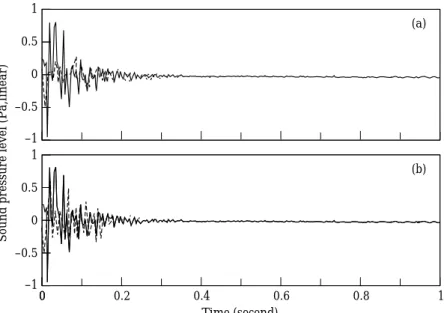
In the final case, an impact noise from a forge hammer in a shipyard was chosen as the primary noise. The reason for choosing the impact noise is because it represents a large class of transient noises. For example, the impact noise of punch presses, the noise of forge
Figure 7. The sound pressure spectra for the blower noise before and after ANC was activated. (a) Modified
H2method; (b) filtered-x LMS method. The step size in the filtered-x LMS was 0·1, the filter length was 256,
0
Sound pressure level (Pa,linear)
0 Time (second) 0.2 (b) 0.5 0 1 –0.5 (a) –1 0.5 0 1 –0.5 –1 0.4 0.6 0.8 1
Figure 8. The time-domain response for the impact noise before and after ANC was activated. (a) Modified
H2method; (b) filtered-x LMS method. The step size used in the filtered-x LMS was 0·05 and the filter length
was 256. ——, Before control; ----, after control.
2 93
machines, the noise of gun shots, and the tunnel noise of high-speed trains all fall into this category. This particular type of application has rarely been investigated in ANC research because it involves difficulties of control methods and transduction. In the study, the authors attempted to use the modified H2method to attack the practical noise problem.
The time-domain response of the impact noise before and after ANC was activated is shown in Figure 8. Visual comparison between the modified H2method and the filtered-x
LMS method indicates that the former produced better performance in suppressing the impact noise than the latter. The filtered-x LMS method appeared sluggish in responding to this transient noise. The allowable adaption time in this case was too short (approximately 0·1 s) for the LMS method which requires the noise be either periodic or with slowly-varying statistics. On the other hand, the H2and Hamethods are essentially
fixed controllers which do not require adaptation and therefore the control of transient noises is almost instant.
5. CONCLUSION
Three feedforward active noise control algorithms based on the H2, the Ha, and the
modified H2 optimal model matching principles have been developed in this study. The
first two methods provide significant noise attenuation for broadband random noises at the expense of the high-gain problem. The third method effectively eliminates the high-gain problem of the ordinary H2 and Ha algorithms. An ANC system for duct noises based
on the feedforward algoithms has been realized by using a digital signal processor. The experimental results indicate that the proposed method provides comparable noise attenuation to the widely-used filtered-x LMS method. In addition, it exhibits great potential in actively suppressing transient noises. A limitation of the proposed method is that the performance will deteriorate if the plant drifts excessively from its normal setting, as may arise in practical applications. From this perspective, the development of adaptive
ANC algorithms based on the H2 and Haprinciples will be the main emphasis of future
research.
ACKNOWLEDGMENTS
Special thanks are due to Professors C. Y. Chung and J. S. Hu for the helpful discussions on the H2 and Ha control theories. The work was supported by the National Science
Council in Taiwan, Republic of China, under project number NSC 83-0401-E009-024.
REFERENCES
1. P. A. N and S. J. E 1992 Active Control of Sound. London: Academic Press. 2. S. J. E and P. A. N 1994 Noise/News International 2, 75–98. Active noise control. 3. D. R. M 1980 IEEE Transactions on Acoustics, Speech, and Signal Processing ASSP-28, 454–467. An analysis of multiple correlation cancellation loops with a filter in the auxiliary path. 4. J. C. B 1981 Journal of Acoustical Society of America 70, 715–726. Active adaptive sound
control in a duct: a computer simulation.
5. J. C. D, B. A. F 1992 Feedback Control Theory. New York: Maxwell-Macmillan International.
6. B. A. F 1987 Lecture Notes in Control and Information Science. A Course in HaControl 88 New York: Springer-Verlag.
7. D. K. M 1991 Journal of Dynamic Systems, Measurements, and Control 113, 419–424. Physical interpretation of transfer function zeros for simple control systems with mechanical flexibilities. 8. K. J. A, P. H, J. S 1984 Automatica 20, 31–38. Zeros of sampled systems. 9. M. M and E. Z 1989 Robust Process Control. Englewood Cliffs, N.J.: Prentice-Hall. 10. G. F. F, J. D. P, and A. E-N 1994 Feedback Control of Dynamic
Systems. Reading, Ma: Addison-Wesley.
11. J. G. P and D. G. M 1992 Digital Signal Processing. New York: Maxwell-Macmillan International.
12. L. L 1987 System Identification: Theory for the User. Englwood Cliffs, N.J.: Prentice-Hall. 13. B. W and S. D. S 1985 Adaptive Signal Processing. Englewood Cliffs, N.J.: