A Pragmatic Labeling Design of MIMO BICM-ID
Systems Based on EXIT Chart
Tsang-Wei Yu and Chung-Hsuan Wang
Department of Communication Engineering,National Chiao Tung University, Hsinchu, Taiwan 30010, Taiwan
[email protected] and [email protected]
Wern-Ho Sheen
Department of Information and Communication Engineering, Chaoyang University of Technology,
Taichung County 41349, Taiwan [email protected]
Abstract—We propose a pragmatic labeling design based on the
extrinsic information transfer (EXIT) chart for bit-interleaved coded modulation with iterative decoding on multiple-input-multiple-output channels. In our design, the EXIT chart is used to determine a candidate set of labelings which have representative demapper transfer curves. Then, a procedure to generate these labelings is provided based on the genetic algorithm. Given fixed channel code and signal-to-noise ratio (SNR), we can search within this candidate set for a most-suitable labeling to minimize the bit-error-rate (BER) with low complexity. Simulation results show that the labeling chosen from the candidate set exhibits a controllable BER performance gap compared to the optimal labeling found through exhaustive search. Besides, even though the channel code or the SNR is changed, the same candidate set can still be directly adopted to reduce the time on re-searching a new labeling.
I. INTRODUCTION
Bit-interleaved coded modulation with iterative decoding (BICM-ID) [1][2] has been shown as an efficient and powerful transmission scheme over fading channels. It was pointed out in [1][2] that different BER performance can be obtained by employing different labelings. Recently, various researches have been done to find out good labelings of the BICM-ID systems for single-input-single-output (SISO) channels [3][4]. For multiple-input-multiple-output (MIMO) channels, single-dimensional labelings are investigated in [5][6], while [7][8] consider more general cases, called multi-dimensional labelings. Part of these works adopt the assumption of error-free feedback from the decoder and the labelings obtained turn out to have good BER performance at high signal-to-noise ratios (SNRs) but experience unacceptable performance loss at low or moderate SNRs.
In fact, it was mentioned in [4] that for any SNR the suitability of a labeling can always be determined with the help of the extrinsic information transfer (EXIT) chart [9], which has been known to be a powerful tool to understand the convergence behavior of iterative decoding schemes. Given a channel code and a fixed SNR, a good labeling should have the information transfer curve of demapper that makes a high first intersection with the decoder curve to allow the trajectory to go as far as possible. However, since any changes of the channel code and SNR may result in variations on the decoder and demapper curves respectively, the desired labeling should
also be different. An intuitive way to keep the optimality is to exhaustively plot the demapper curves of all possible labelings on the EXIT chart to find a new one whenever the channel code or SNR is changed. Obviously, the complexity of such an exhaustive search turns out to be infeasible, especially for large number of transmit antennas and large constellations. To reduce the search complexity, the binary switch algorithms (BSA) are employed in [4] for labeling searching.
In this paper, a pragmatic methodology for labeling design is presented to accommodate the impact of different channel codes and SNRs. Based on the EXIT chart, an observation shows that for the demapper transfer curves that have similar shapes and similar values on their left and right end points, their corresponding behavior on the BER performance, includ-ing the occurrence of the waterfall region and the BER of the error floor region, are usually similar [10]. Therefore, we can first partition all possible labelings into groups according to their values of two end points and then choose a representative labeling from each group to form a set, called the candidate set. As long as the channel code and SNR are given, we can search within the candidate set for a most-suitable labeling with low search complexity. To practically generate the candidate set, a procedure is proposed based on the genetic algorithm (GA) [11]. Simulation results shows that the labeling we chosen from the candidate set can exhibit a controllable BER performance gap compared to the optimal labeling found through exhaustive search. Besides, even though the channel code or the SNR is changed, the same candidate set still can be directly adopted to reduce the time on re-searching a new labeling.
The rest of this paper is organized as follows. In Section II the system model of MIMO BICM-ID is given as well as the basic guideline of labeling design based on the EXIT chart. The idea of the candidate set and the procedure for generating the set are presented in Section III. In Section IV, simulation results are provided to verify the validity of our design for different channel codes and SNRs. Finally, a conclusion is drawn in Section V.
II. SYSTEMMODEL ANDEXIT CHARTBASEDANALYSIS
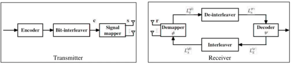
Consider the system model of MIMO BICM-ID with NT transmit antennas and NR receive antennas as shown in Fig.
Transmitter Receiver
Fig. 1. Block diagram of BICM-ID systems.
1. A binary sequence c = [c0, ..., cmNT−1] generated by an
encoder C and an interleaver is first mapped to a vector
s = [s1, ..., sNT]
T by a labeling µ, where s
n is drawn from a regular constellation χ with 2msignal points, ∀ 1 ≤ n ≤ N
T. For single-dimensional labelings,c is first partitioned into NT groups and then each group is mapped to a scalar signal point sn before de-multiplexed to transmit antennas. Here, we consider multi-dimensional labelings [7] which directly
map c to s. The signal vector s is then transmitted through
a frequency-nonselective MIMO channel, and the received signalr = [r1, ..., rNR]
T can be expressed as
r = Hs + w, (1)
where the channel gain H is an NR × NT matrix with each element being identical independent complex Gaussian distribution of zero mean and unit variance and the noise w
is an NR× 1 vector in which the elements are zero-mean complex Gaussian random variables with variance N0/2 per dimension.
The receiver is divided into two main blocks: the demapper and the decoder. Upon receivingr, the demapper φ takes r as
well as L(φ)
A (ci)’s, the a priori inputs of coded bits feedback from the decoder ψ to computes the extrinsic log-likelihood ratios (LLRs) L(φ) E (ci)’s according to L(φ)E (ci) = ln P s∈κ1 i exp ( −kr−Hsk 2 N0 + P j6=i cjL (φ) A (cj) ) P s∈κ0 i exp ( −kr−Hsk 2 N0 + P j6=i cjL(φ)A (cj) ) , (2) where κ0
i and κ1i denote the sets consisting of all the s’s for which the corresponding ci is of binary value 0 and 1, respectively. These extrinsic outputs of demapper are then de-interleaved and taken by the decoder as the a priori inputs L(ψ)A (ci)’s. By an appropriate soft-input soft-output decoding algorithm, e.g. the BCJR algorithm [12], the decoder generates the extrinsic LLRs L(ψ)
E (ci)’s and passes them back to the demapper for further iterations of decoding.
To trace the effect of µ on MIMO BICM-ID, we use the EXIT chart for performance analysis on account of its iterative processing nature. By evaluating the mutual infor-mation between LLRs and the coded bits, two inforinfor-mation transfer curves Φµ(·) and ΨC(·) are plotted in the EXIT chart to describe how the input information I(φ)
A and I (ψ) A are transferred to the output information I(φ)
E and I (ψ) E by the demapper φ and decoder ψ respectively, i.e.
IE(φ)= Φµ(IA(φ)) and I (ψ)
E = ΨC(IA(ψ)). (3)
Note that Φµ(·)is also a function of the SNR, though we omit the corresponding parameter of SNR for simplicity. We also define the two end points of the demapper curve by
αµ = Φµ(0) and βµ= Φµ(1). (4) Let pµ,C denote the first intersection of the demapper and decoder curves, i.e. the smallest mutual information that makes Φµ(I) = Ψ−1C (I). According to the EXIT chart, the BER of BICM-ID systems after a sufficient iterations is determined by pµ,C. Since a labeling that achieves a higher value of pµ,C is able to provide a lower BER, intuitively, one can always obtain a labeling which can achieve the lowest BER by exhaustive search such that
µ∗
C= arg max
µ∈Upµ,C, (5)
where U denotes the set of all possible labelings.
III. PRAGMATICDESIGNMETHODOLOGY OFLABELING
WITHLOWSEARCHCOMPLEXITY
The exhaustive search in (5) can always guarantee the lowest BER at a fixed channel code and a fixed SNR. However, since the decoder curve depends on the channel code and the demapper curve varies with the SNR, to the best of our knowledge there does not exist an universal labeling of regular modulation that is optimal for all channel codes and SNRs. An intuitive way to keep the optimality is to perform (5) whenever the channel code or the SNR is changed. Obviously, the corresponding search complexity becomes infeasible as m or NT increases. Although algorithms, such as BSA, can be used to speed up the search time, the resulting complexity is still high if the channel code or the SNR is changed frequently. Besides, given fixed channel code and SNR, we observe that the labelings with similar values of αµ’s and βµ’s, will usually have similar BER performance. (Here, the BER performance includes the SNRs where the waterfall regions occur and the BERs of the error floor regions.) Therefore, we may be able to perform a more efficient search if we can avoid trying the demapper curves with similar shapes.
Motivated by above two reasons, an intuitive idea is to first partition all possible labelings into N groups according to the similarity of their αµ’s and βµ’s. Then one representative labeling is picked from each group to form a set of labelings, call the candidate set Γ. Once the channel code and the SNR are known, the labeling can then be selected within Γ by
µΓC= arg max
In this way, we can both reduce the search complexity by controlling N, the number of labelings in Γ, and avoid trying demapper curves with similar shapes. However, it is infeasible to plot the demapper curves of all possible labelings on the EXIT chart, especially for large m and NT. Therefore, to obtain Γ in practice, we would like to first determine the desired values of αµ’s and βµ’s we need in Γ, and then find corresponding labelings to approach these values. Let µ0 denotes the Gray labeling, which is known as the one with the largest αµ and smallest βµ among all labelings. Now the procedure for generating Γ is listed as following:
Procedure for generating Γ:
Step 1: Use GA to find the labeling with the largest βµ−αµ. Denote this labeling by µN −1 and let n = 0. Step 2: Let δα= αµ0−αµN N −1 and δβ= βµN−βµ0 N −1 . Let α∗ k = αµ0− k ∗ δα and β ∗ k = βµ0+ k ∗ δβ, ∀k = 1, 2, ..., N − 2.
Step 3: Let n = n + 1 and use GA to find the labeling µnthat minimizes the fitness function θn(µ), where θn(µ) = |α∗n− αµ| + |βn∗− βµ|
Step 4: If n = N − 1,
Let Γ={µ0, µ1, ..., µN −1}and stop the procedure. Else, go back to Step. 3.
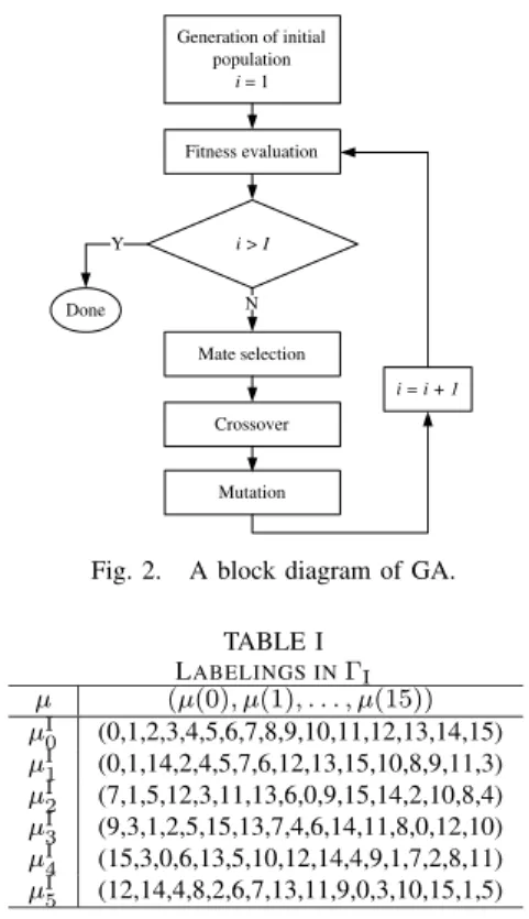
Following the procedure, we can successively obtain new labelings with decreasing αµ’s and increasing βµ’s. In Step. 1 and 3, the labeling is found according to the genetic algorithm [11] shown as Fig. 2. Firstly, a set of labelings are randomly generated as the initial population with P members. Secondly, the fitness function θ(µ) of each labeling in the population is evaluated and the first P/2 labelings with smaller θ(µ)’s are kept, while the others are eliminated. Note that only αµ and βµ of each labeling are needed to be calculated here. Then, a pair of labelings are randomly selected to carry out the crossover, where the label on each signal point of one is randomly decided with probability 0.5 whether or not to adopt the label of its mate to create an offspring. Every offspring has a probability of q to suffer a mutation, where two randomly-selected signal points on the constellation exchanges their labels. Sufficient pairs are picked until the total number of the survivors and the offsprings equals P . After that, a new iteration will start from the re-evaluation of the fitness functions. The GA will stop until I iterations have been done. Instead of BSA, GA is chosen in our design because that the randomly-generated initial population can make the search efficiency less depend on the initial labelings and that the mutation step is more likely to get the solutions out of local optimums.
Examples of the candidate sets ΓIand ΓIIfor SISO 16QAM are given in Table I and Table II with N = 6 and 10 respectively, wherein the Gray labeling is used as the indexing of the signal points and the decimal representation is used for the binary labels. The labelings in the tables are listed in a decreasing order in terms of their αµ’s and their corresponding curves are plotted in Fig. 3(a) and Fig. 3(b) with Es/N0= 6 dB at AWGN channels. Using large N is able to create a
Generation of initial population i = 1 Fitness evaluation i > I Mate selection Crossover Mutation N Y Done i = i + 1
Fig. 2. A block diagram of GA. TABLE I LABELINGS INΓI µ (µ(0), µ(1), . . . , µ(15)) µI 0 (0,1,2,3,4,5,6,7,8,9,10,11,12,13,14,15) µI 1 (0,1,14,2,4,5,7,6,12,13,15,10,8,9,11,3) µI 2 (7,1,5,12,3,11,13,6,0,9,15,14,2,10,8,4) µI 3 (9,3,1,2,5,15,13,7,4,6,14,11,8,0,12,10) µI 4 (15,3,0,6,13,5,10,12,14,4,9,1,7,2,8,11) µI 5 (12,14,4,8,2,6,7,13,11,9,0,3,10,15,1,5) .
candidate set with smaller δα and δβ. (Note that although Gray labeling is not unique, using different Gray labelings on indexing the signal points in our tables will lead to identical set of demapper curves.) Once the SNR and the channel code are known, the labeling can then be select within ΓI or ΓII according to (6). Note that the number of labelings needed to be compared is extremely reduced from 16! (in (5)) to 6 or 10. For the MIMO case, a candidate set ΓIII for BPSK with NT = NR= 4on MIMO Rayleigh fading channels with Es/N0= −1dB is listed with the same order in Table III and the corresponding curves are plotted in Fig. 4. The number of labelings needed to be compared is extremely reduced from 16!to 10 in ΓIII. Note that the candidate sets are obtained by setting I = 30, P = 30, and q = 0.05. Further increasing I or P brings only trivial improvement on the minimum θn(µ) among the populations, according to our experience from experiments. TABLE II LABELINGS INΓII µ (µ(0), µ(1), . . . , µ(15)) µII 0 (0,1,2,3,4,5,6,7,8,9,10,11,12,13,14,15) µII 1 (0,1,2,3,4,5,6,7,8,9,15,11,12,13,10,14) µII 2 (1,4,2,6,0,5,3,7,9,8,11,10,12,13,14,15) µII 3 (1,0,2,3,4,5,14,7,8,11,10,9,12,13,6,15) µII 4 (9,15,12,14,11,1,8,2,5,4,3,6,13,7,10,0) µII 5 (12,14,4,8,2,6,7,13,11,9,0,3,10,15,1,5) µII 6 (1,13,15,5,11,9,3,12,2,4,7,0,8,14,6,10) µII 7 (5,9,15,3,0,2,6,12,8,1,4,7,10,11,14,13) µII 8 (15,11,1,2,6,8,7,4,0,9,10,3,5,12,13,14) µII 9 (4,14,9,3,7,13,10,0,2,8,15,5,1,11,12,6) .
TABLE III LABELINGS INΓIII µ (µ(0), µ(1), . . . , µ(15)) µIII 0 (0,1,2,3,4,5,6,7,8,9,10,11,12,13,14,15) µIII 1 (8,0,2,10,4,12,6,14,1,9,3,11,5,13,7,15) µIII 2 (8,0,2,10,4,12,14,6,1,9,3,11,5,13,7,15) µIII 3 (1,0,2,3,4,5,7,6,9,8,11,10,12,13,14,15) µIII 4 (8,4,2,10,0,12,14,6,1,9,11,3,5,13,7,15) µIII 5 (1,13,6,15,5,8,2,10,4,9,3,14,0,12,7,11) µIII 6 (2,13,6,9,5,8,1,15,4,10,3,14,0,12,7,11) µIII 7 (0,15,7,9,5,8,10,13,4,1,3,14,2,12,6,11) µIII 8 (8,15,7,9,5,0,10,13,6,1,11,14,2,12,4,3) µIII 9 (15,4,0,11,2,9,13,6,1,10,14,5,12,7,3,8) 0 0.2 0.4 0.6 0.8 1 0 0.1 0.2 0.3 0.4 0.5 0.6 0.7 0.8 0.9 1 I(φ) A I (φ ) E (a) 0 0.2 0.4 0.6 0.8 1 0 0.1 0.2 0.3 0.4 0.5 0.6 0.7 0.8 0.9 1 I(φ) A I (φ ) E (b)
Fig. 3. The demapper transfer curves of (a) ΓIin Table I and (b) ΓII in
Table II with Es/N0= 6dB at AWGN channels.
IV. SIMULATIONRESULTS
For SISO 16QAM, the examples of labeling selection in ΓII are given in Fig. 5(a) and Fig. 5(b) for BCJR decoder of convolutional code with with generator matrix (1 + D + D2+ D3, 1 + D + D3), denoted by CC(17,15) for simplicity, and AWGN channels with Eb/N0= 3 dB and 4 dB, respectively. For Eb/N0 = 3 dB, the labeling that achieves the highest first intersection is µII
6, while for Eb/N0= 4dB, µII9 becomes a favorable choice. The optimality of µII
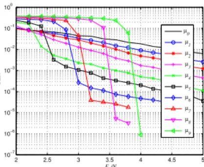
6 and µII9 among ΓII for the two different SNRs can be easily verified by the BER simulation in Fig. 6, wherein a bit-interleaver of block length 80000 bits, an MAP demapper in (2) and a BCJR decoder are employed for iterative decoding with 40 iterations. It can also be observed that on one hand the labelings µ0, µ1, ..., µ9 which have an order of regularly decreasing αµ can result in increasing SNRs of the occurrence of the waterfall regions and on the other hand the order of regularly increasing βµ also leads to a regularly decreasing BERs at the error floors.
0 0.2 0.4 0.6 0.8 1 0 0.1 0.2 0.3 0.4 0.5 0.6 0.7 0.8 0.9 1 I(φ) A I (φ ) E
Fig. 4. The demapper transfer curves of ΓIIIin Table. III with Es/N0= −1
dB at Rayleigh fading channels.
0 0.2 0.4 0.6 0.8 1 0 0.1 0.2 0.3 0.4 0.5 0.6 0.7 0.8 0.9 1 I(φ) A, I (ψ) E I (φ ) E , I (ψ ) A CC(17,15) (a) 0 0.2 0.4 0.6 0.8 1 0 0.1 0.2 0.3 0.4 0.5 0.6 0.7 0.8 0.9 1 I(φ) A, I (ψ) E I (φ ) E , I (ψ ) A CC(17,15) (b)
Fig. 5. EXIT chart with the transfer curves of decoder CC(17,15) and the demapper curves in ΓII for AWGN channels with (a) Eb/N0 = 3dB (b)
Eb/N0= 4dB.
Besides, each labeling is favorable at its own SNR interval and thus we can directly adopt this candidate set on different SNRs to reduce the time on re-searching a new labeling using BSA or exhaustive search. For the MIMO case, the BER simulations of labelings in ΓIII are shown in Fig. 7 for BCJR decoder of convolutional code with with generator matrix (1 + D + D2, 1 + D2) and Rayleigh fading channels. It can also be observed that it is beneficial to select proper labelings from ΓIII on individual SNR intervals, though the EXIT charts to illustrate the corresponding selection are omitted here due to the length limitation.
Fig. 8 shows the effect of N on the labeling selection. The labelings µI
3 and µII6 are chosen from ΓI (N = 6) and ΓII (N = 10) respectively to achieve the highest first intersection with the decoder curve of BCJR decoder of CC(17,15), while the labeling µ∗
2 2.5 3 3.5 4 4.5 5 10−7 10−6 10−5 10−4 10−3 10−2 10−1 100 Eb/N0 BER µ0 µ1 µ2 µ3 µ4 µ5 µ6 µ7 µ8 µ9
Fig. 6. The BER performance of the candidate set ΓIIfor Table. II at AWGN
channels. 1 2 3 4 5 6 10−6 10−5 10−4 10−3 10−2 10−1 100 Eb/N0 BER µ II 0 µ II 1 µ II 2 µ II 3 µ II 4 µ II 5 µ II 6 µ II 7 µ II 8 µ II 9
Fig. 7. The BER performance of the candidate set ΓIIIfor Table. III at fast
Rayleigh fading channels.
GA. It is shown in Fig. 8 that µ∗
C has the highest intersection, closely followed by µII
6 and then µI3 at Eb/N0 = 3 dB. The corresponding BER performance in Fig. 9 sustains the observations in Fig. 8. Usually, the labeling chosen from the candidate with large N is more likely to achieve close BER performance to the BER performance of µ∗
C. In our case, N = 10 is good enough to have the close-to-optimum BER performance, while the number of labelings needed to be compared is extremely reduced to 10.
V. CONCLUSION
A pragmatic design of labeling for MIMO BICM-ID is presented in this paper with the help of the EXIT-chart based analysis. To both reduce the search complexity and avoid trying labelings with similar shapes, the idea of the candidate set is first specified on the EXIT chart and realized by a procedure based on GA. Once the channel code and SNR are known, we can search within the candidate set for a most-suitable labeling to achieve the lowest BER with low complexity. Simulation results show that the labeling chosen from the candidate can achieve a very close BER performance to the labeling obtained by exhaustive search. Besides, even though the channel code or the SNR is changed, the same candidate set still can be directly adopted to reduce the time on re-searching new labelings using BSA or exhaustive search.
REFERENCES
[1] A. Chindapol and J. A. Ritcey, “Design, analysis, and performance evaluation for BICM-ID with square QAM constellations in Rayleigh-fading channels”, IEEE J. Select. Areas Commun., vol. 19, pp. 944-957, May 2001. 0 0.2 0.4 0.6 0.8 1 0 0.1 0.2 0.3 0.4 0.5 0.6 0.7 0.8 0.9 1 I(φ) A, I (ψ) E I (φ ) E , I (ψ ) A CC(17,15) µ I 3 µ II 6 µ * C
Fig. 8. EXIT chart with the transfer curves of decoder CC(17,15)
and the demapper curves of labelings µI 3, µ II 6 and µ∗C with µ∗C = (14, 13, 0, 4, 7, 8, 5, 1, 9, 15, 3, 10, 11, 2, 6, 12). 2 2.5 3 3.5 4 4.5 10−5 10−4 10−3 10−2 10−1 100 Eb/N0 BER µ I 3 µ II 6 µ* C
Fig. 9. The BER performance of the labelings µI 3, µ
II
6 and µ∗C at AWGN
channels, note that the curve of µ∗
C at Eb/N0 = 3dB is obtained by
performing 80 iterations.
[2] X. Li, A. Chindapol and J. A. Ritcey, “Bit-interleaved coded modulation with iterative decoding and 8PSK signaling,” IEEE Trans. Commun., vol. 50, Aug. 2002.
[3] J. Tan and G. L. Stuber, “Analysis and design of symbol mappers for iteratively decoded BICM,” IEEE Trans. Wireless Commun., vol 4, pp. 662-672, Mar. 2005.
[4] Q. Cheng, X. Xu, S. Zhou and L. Xiao, “A new labeling search method for bit-interleaved coded modulation with iterative decoding,” in Proc.
IEEE VTC 2005-Spring Conf., Stockholm, Sweden, May, 2005, pp
587-590.
[5] Y. Li and X. G. Xia, “Constellation mapping for space-time matrix modu-lation with iterative demodumodu-lation/decoding,” IEEE Trans. Commun., vol. 53, pp. 764-768, May 2005.
[6] A. Sezgin and E. A. Jorswieck, “Impact of the mapping strategy on the performance of APP decoded space-time block codes,” IEEE Trans.
Signal Process., vol. 53, pp. 4685-4690, Dec. 2005.
[7] N. H. Tran and H. H. Nguyen, “Design and performance of BICM-ID systems with hypercube constellations,” IEEE Trans. Wireless. Comm., vol. 5, no. 5, pp. 1169-1179, May. 2006.
[8] F. Simoens, H. Wymeersch, H. Bruneel and M. Moeneclaey, “Multi-dimensional Mapping for Bit-Interleaved Coded Modulation with BPSK/QPSK Signaling,” IEEE Comm. Lett., vol. 9, no. 5, May 2005. [9] A. Ashikhmin, G. Kramer, and S. ten Brink, “Extrinsic Information
Transfer Functions: Model and Erasure Channel Properties,” IEEE Trans.
Inform. Theory, vol. 50, pp. 2657-26733, Nov. 2004.
[10] T. Clevorn, S. Godtmann, and P. Vary, “BER prediction using EXIT Chart for BICM with Iterative Decoding,” IEEE Comm. Lett., vol. 10, pp. 49-51, Jan 2006.
[11] E. K. P. Chong and S. H. Zak, An introduction to optimization. John Wiley and Sons, 2001.
[12] L. R. Bahl, J. Cocke, F. Jelinek and J. Raviv, “Optimal decoding of linear codes for minimizing symbol error rate,” IEEE Trans. Inform. Theory, vol. 20, pp.284-287, Mar. 1974.