下一代多層級多媒體應用服務匯流網路－總計畫:下一代多層級多媒體應用服務匯流網路(2/3)

行政院國家科學委員會專題研究計畫 期中進度報告

下一代多層級多媒體應用服務匯流網路--總計畫:下一代多

層級多媒體應用服務匯流網路(2/3)

期中進度報告(精簡版)

中 華 民 國 96 年 06 月 20 日

行政院國家科學委員會專題研究計畫 期中進度報告

中華民國

96 年 6 月 6 日

總計畫:下一代多層級多媒體應用服務匯流網路(2/3)

行政院國家科學委員會補助專題研究計劃

下一代多層級多媒體應用服務匯流網路-總計畫：下一代多層級多媒體應用服務

匯流網路(2/3)

Next Generation Multi-layer Multimedia Service Convergence Network

計畫編號：NSC 95-2221-E-002-199 執行期限：95年8月1日至96年7月31日 計畫主持人：國立臺灣大學電信工程研究所 蔡志宏 教授 共同主持人：國立臺灣大學電信工程研究所 張時中 教授 國立臺灣大學電信工程研究所 林宗男 副教授 國立臺灣大學資訊管理學系 孫雅麗 教授 一、中英文摘要 隨著資訊科技的進展，網際網路傳輸 的內容早已由文字進展至多媒體，並擴及 語音及視訊，多媒體應用與通訊服務的整 合需求已成為未來科技的研發指標。可是 現有網際網路及未來無線網際網路在速 度、品質及安全上仍有很大改善空間，支 援QoS 服務仍是一大挑戰。 本計畫所提之研究題目，〝下一代多 層級多媒體服務匯流網路〞乃針對多重服 務下QoS 保障及資源管理的挑戰而訂， 以應付未來無線/有線寬頻網路，快速進 展的串流多媒體，以及固定/行動服務匯 流趨勢。 雖然議題眾多，我們仍選擇幾項重點 基礎技術項目投入，為解決無線網狀網路 的QoS 需求，我們研究其多媒體服務之 移動及資源管理；為使內容傳遞之疊加網 路有效運用資源，我們投入研究其關鍵先 進技術；有效率共享頻率及共享骨幹寬 頻，我們建議採用可重組及支援QoS 之 服務匯流網路架構；最後我們將整合服務 及計算資源之分散式視訊偵搜網路訂為 應用層之典型應用加入研究。 本報告為此三年期計畫中之第二年 成果報告，將就以上領域提出四大子計畫 之成果貢獻。 關鍵詞：無線網狀網路、多媒體服務、 資源分配、疊加網 Abstract:

As the rapid development of information technologies, the transmission contents over the Internet change from pure text to multimedia data, including VoIP and video. The integrating need of multimedia application and network communication services has become the guide of the future technology developments. However, the existing Internet architecture and the emerging wireless Internet still has some improvement space considering the transmitting speed, quality of service, and security. Supporting Quality-of-Service

(QoS) in the Internet remains a very challenging task.

The proposed research topic, the Next Generation Multi-layer Multimedia Service Convergence Network, is thus to meet the QoS assurance and resource management challenges of various services and applications that may arise in the future wireless/wired broadband network, as we embrace the fast advance of streaming multimedia applications and recent trend of fixed/wireless service convergence.

Although such an architecture involves a very sophisticated integration of services and technologies, we choose to study the following fundamental technologies first. In order to resolve the QoS service requirement in the emerging wireless mesh network, we study its resource and mobility management for multimedia services. To provide efficient use of resource for content delivery overlay network, we investigate several advanced technologies of overlay networks. For efficient spectrum and shared infrastructure resource sharing in the service convergence era, we suggest to study the Next Generation Service Convergence Network Architecture, with QoS and Re-configuration Capability. Last but not least, we include the distributed video surveillance in an Integrated Computation and Network Services environment, as the application layer topic.

This report is a research summary for

the 2nd year study in the 3-year project, and we shall provide a summarized contribution obtained in the 4 key sub-projects.

Key words: QoS, service convergence,

wireless mesh network, multimedia services, resource allocation, overlay network

二、研究方法、結果與討論

2.1 子計畫一：在無線網狀網路支援多媒

體服務的資源與移動管理

2.1.1 研究目標

The wireless mesh network (WMN) is quickly emerging as a promising complementary solution to existing broadband access infrastructure. An important performance metric to evaluate the effectiveness of such a network is the "“network capacity throughput＂ which is defined as the aggregate number of bits that can be received under certain quality requirement by designated receivers in the network for a certain period of time. To maximize the capacity throughput of a wireless mesh network, it is essential to explore the maximal number of concurrent transmissions in the network. Different from single point to point transmissions (e.g., wireless LAN), in a WMN the interference between mesh nodes (SSs) is an important factor in determining the network capacity throughput that place more challenges to the design of medium access protocol.

2.1.2 研究方法與步驟

We consider a WMN employing a Time Division Multiple Access (TDMA)

based scheduling scheme similar to the coordinated distributed scheduling as defined in [1]. We assume all SSs are equipped with omni-directional antennas, use single channel, and all SSs transmit at the same power level.

2.1.2.1 The Network Model

In a WMN, a condition must be satisfied for a successful wireless transmission. It’s that the signal to interference plus noise ratio (SINR) at receiver must be no smaller than its capture threshold denoted as CPThresh. This is referred to as the capture threshold constraint.

For the wireless communications, the physical interference model and the spectral efficiency (the sustainable transmission rate per Hz bandwidth) model similar to those proposed in [2][3][4][5] are assumed. Under the physical model, the signal quality (SINR) of a TX/RX pair is given as follows:

( ) ( ) ∑ ∑ = <−> > − < = −> > − + = + = _|| 1 | | 1 I i IF RX IF RX TX TX I i IF RX RX TX i i i _d P Noise d P ce Interferen Noise Signal SINR α α

where PTX is the transmitter power of station TX, dTX<->RX is the distance between stations TX and RX, and α is the path-loss exponent which is a parameter of the environmental condition of the deployed WMN. Its typical range is between 2.0 to 6.0 [6]. PIFi is the transmitter power of transmitter IFi, dIFi<->Non_Intended_RX is the distance between the interfering transmitter and the non-intended receiver, and |I| is the number of the other concurrent transmissions in the same slot.

2.1.2.2 Network Utilization – Transmission Concurrency and Spectral Efficiency

To maximize the network capacity throughput, an effective approach is to exploit spatial channel reuse and obtain the maximal number of concurrent transmissions at each time slot.

Let ρ represent the network utilization which is defined as the ratio of the total transmission pairs scheduled to the maximum number of possible transmission pairs in a data time slot in the wireless mesh network.

∑

Let Tnet(l) represent the network capacity throughput at time slot l which is the sum of the individual link rate (or the transmission spectral efficiency) that are scheduled to transmit in the slot, i.e.

duration timeslot data transPairs SpecEff l T num pair scheduled onPair Transmissi net _{_ _} * ) ( _

∑

There is a tradeoff between the transmission spectral efficiency employed by individual links and the number of concurrently schedulable (successful) transmission pairs. Basically, to allow more number of schedulable concurrent transmissions, one would need to reduce individual transmission’s spectral efficiency. On the other hand, if a transmitter increases its transmission spectral efficiency, the total number of schedulable concurrent transmission pairs must be limited to avoid unnecessary interference.

Clean-Air Policy to produce a feasible

channel access schedule of the data time slots that meets the target ρ. An algorithm will be proposed to properly assign transmission spectral efficiencies to each transmit/receive pair in the schedule to satisfy individual receiver’s capture threshold constraint. Then, the resulting network capacity throughput is calculated.

2.1.2.3 Data Slot Scheduling

We group a certain SS’s (SSi)

neighboring SSs into different groups. The SSs that physically closest (distance to SSi

is less than a threshold value) to SSi are

referred to as the tier-1 neighbors of SSi.

The tier-1 neighbors of an SS’s tier-1 neighbors are referred to as its tier-2 neighbors.

The TDMA frame structure is similar to the mesh mode frame structure in [1]. Each frame consists of a control subframe and a data subframe. The control subframe is comprised of multiple fixed-size control message transmission opportunities and the data subframe consists of multiple fixed-size data slots which are used for data transfer after the connections have been established. We use the three-way-handshake connection setup scheme as our data slots access protocol. First, a transmitter SST will send a

REQUEST message in the control subframe to the intended receiver SSR which carries

SST’s data subframe slot availability

information in the next N frames. SSR then

compares its own data subframe slot availability information with sender’s

information and responds with a GRANT (also in control subframe) message indicating the set of the data subframe slots that are available to receive. Finally, if agreed, SST will send a CONFIRMATION

message (also in control subframe) to SSR.

After agreeing upon the transmission schedule, SST and SSR will not let these

reserved data subframe slots to be reserved again by other SSs. Then, SST will send

data packets to SSR on the granted data

subframe slots.

Based on the three-way-handshake scheme, we propose the “Tier-k Clean-Air

Policy” to explore which spatial reuse

policy can achieve maximal network capacity throughput. The “Tier-k Clean-Air

Policy” states that at each data slot, for

every SS that is scheduled to transmit (receive), all its tier-1, tier-2 and up to tier-k neighbors except for the intended receiver (sender), must not be scheduled to transmit or receive. We also define a special case referred to as the tier-0 clean-air condition. Under the condition, for every SS scheduled to transmit, all of its tier-1 neighbors, except for the intended receiver, are only prohibited from receive at the same time. But they are allowed to transmit so long as

(a) ρ = 1 (b) ρ = 1/2 (c) ρ = 1/3

Fig. 1. Example transmission patterns that satisfy tier-0, tier-1 and tier-2 clean-air conditions.

their transmission does not affect this transmit/receive pair. Likewise, for every SS scheduled to receive on a data slot, all its tier-1 neighbors, except for the target transmitter, are prohibited from transmit simultaneously. Figure 1(a) shows an example of tier-0 clean-air policy in which all SSs are either transmitting or receiving. Hence, this transmission pattern has 100% network utilization. Figure 1(b) and 1(c) depict two example transmission patterns of the tier-1 and tier-2 clean-air conditions, achieving 50% (i.e. one half of the total SSs are either transmitting or receiving) and 33% network utilization, respectively.

2.1.2.4 Schedulers that implement “Tier-k Clean-Air Policy” with given network utilization ρ

Given a target ρ in a data slot and the tier-k clean-air policy, next step we will find an algorithm that can generate an appropriate control/data subframe access schedule and appropriate spectral efficiencies of every transmission that meets the target ρ while satisfying the tier-k clean-air spatial reuse condition. Different policies are with different network utilization and degree of interference. We explore the network capacity throughput that can be achieved by tier-0/tier-1/tier-2 policies. To evaluate the performance, first we will assume regular hexagonal topology of the WMN with always backlogged SSs to explore which policy gives the maximum network capacity throughput. Second we examine the impact of realistic deployment scenario by introducing random

perturbations to mesh SSs. Third, instead of assuming all SSs are backlogged, we randomly add traffic to different pairs of stations to explore which policy gives the maximum network capacity throughput.

2.2 子計畫二：下一代多層級多媒體服務

匯流網路之疊加層網路關鍵技術

2.2.1 研究目標

The design of search algorithms is critical to the performance of unstructured peer-to-peer (P2P) networks [7]. In the unstructured P2P networks, each node does not have the global information about the whole topology and the location of queried resources. Because of the dynamic nature of unstructured P2P networks, it is also difficult to correctly capture the global behavior [8] [9]. Therefore, it depends on the search algorithms to help locating the queried resource and routing the message to the target node.

Previous works about the search issue in unstructured P2P networks can be classified into two categories: breadth first search (BFS)-based methods, and depth first search (DFS)-based methods. These two types of search algorithms tend to be inefficient, either generating too much load on the system [10][11], or not meeting users’ requirements[12].

In this project we propose the dynamic search algorithm (DS) which is a generalization of flooding and RW. DS overcomes the disadvantages of flooding and RW, and takes advantage of different contexts under which each search algorithm performs well. The operation of DS

resembles flooding for the short-term search and RW for the long-term search.

2.2.2 研究方法與步驟

2.2.2.1 Operation of Dynamic Search Algorithm

DS is designed as a generalization of flooding, MBFS, and RW. There are two phases in DS, and each phase has different searching strategy. The choice of search strategy at each phase depends on the hop count h _{of the query messages and the}

decision threshold n _{of DS.}

Phase 1. When h n≤ :

At this phase, DS acts as flooding or MBFS. The number of neighbors that the query source sends the query messages to depends on the pre-defined transmission probability p. If the link degree of this

query source is d, it would only send the

query messages to d p⋅ neighbors. When

p is equal to 1, DS resembles flooding.

Otherwise it operates as MBFS with transmission probability p.

Phase 2. When h n> :

At this phase, the operation of DS switches to RW. Each node which receives the query message would send the query message to one of its neighbors if it does not have the queried resource. Assume that the number of nodes visited by DS at hop h n= is the coverage c_n, and

then the operation of DS at that time can be regarded as RW with c_n walkers. Fig. 1

shows the pseudocode of DS.

In short, DS is designed to perform aggressively in short-term search, and conservatively in long-term search.

Obviously the parameters n _and p

would affect the performance of DS.

2.2.2.2 Knowledge-based Dynamic Search

Some knowledge-based search algorithms, including APS, biased RW, RI, local indices, and intelligent search, are applicable to combine with our DS algorithm, and any training or caching operations benefit from our DS algorithm as well. In this subsection we present the generic scheme to incorporate these knowledge-based search algorithms with our DS algorithm. We construct the probabilistic function based on the information learned from the past experiences, with respect to each search target, search time, and local topology information. Thus a node has more information to intelligently decide how many query messages to send and to which peers these messages should be forwarded. Take APS as an example. The peer

Fig. 1. The pseudocode of DS algorithm. Algorithm: The pseudo-code of dynamic search DS

Input: query source s, queried resource f, transmission probability p Output: the location information of f

DS(s, f, p)

/* the operation of s */

h ← 0

if (h <= n)

h ← h + 1

s choose p portion of its neighbors mi carring h visits these chosen neighbors

elseif (h > n)

h ← h + 1

mi carring h visits one neighbor of s

applying APS search builds a probability table for each neighbor and each object. It consistently refines its probability table by the search experiences. If a search query for some object delivers to certain neighbor successfully, the probability entry corresponding to that neighbor and object is increased. If the search fails finally, it will decrease the probability entry. In accordance with APS, when a certain node receives a hit from peer i, it adds 10 points for the entry of peer i; if peer i fails to respond the hit to that node, the node subtracts 10 points for the entry of peer i.

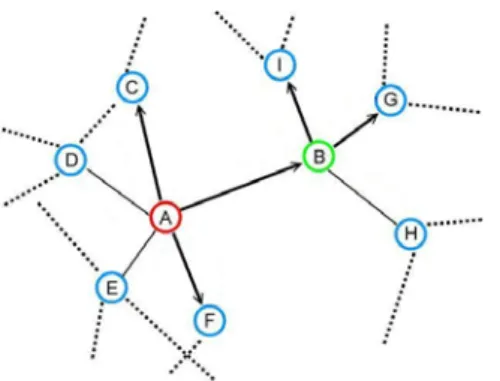
Fig. 2 shows an example of knowledge-based DS algorithm. Node A initializes a search for a certain object. It makes its forwarding decision of which neighbors should be sent to in accordance with the probability table shown in TABLE 1. Assume the messages are sent to node B, C, F. When node B receives the message, it checks its probability table shown in TABLE 1 and generates another two query messages to node I and G.

We apply Newman’s random graph as the network topology, adopt the generation functions to model the link degree distribution [13], and analyze DS based on

some performance metrics, including the success rate, search time, query hits, query messages, query efficiency, and search efficiency. The analysis by generating functions talks about a graph all of whose parameters are exactly what they should be on an average random graph.

2.2.2.3 Performance Metrics

Success rate (SR_{) is the probability}

that the query is success, i.e., there is at least one query hit. Assume that the queried resources are uniformly distributed in the network with a replication ratio R _of

the queried object, and then SR _{can be}

calculated as ( ) 1- 1- C

SR= R

where R _{is the replication ratio and} C _is

the coverage.

To represent the capability of one search algorithm to find the queried resource in time with a given probability, we define the search time (ST_{) as the search}

time it takes to guarantee the query success with success rate requirement SRreq_. ST

represents the hop count that a search is successful with a probabilistic guarantee.

ST _{for DS is}

Fig. 2. Illustration for the operation of knowledge-based DS algorithm.

TABLE1.

A. Probability table for node A.

Node C D E B F

Prob. 0.78 0.12 0.04 0.85 0.92 B. Probability table for node B.

Node G H I - -

( )

(

)

( )

(

)

(

)

(

)

(

)

( )

The number of query hits QH and the number of query messages QM are the well-known performance metrics for the evaluations of search algorithms. Generally speaking, the objective of search algorithms is to get the most query hits with the fewest query messages, but these two metrics often conflict with each other. Therefore, it requires a more objective metric to evaluate the search performance. We adopt the performance metrics proposed in [14], query efficiency (QE) and search qfficiency (SE_{), which consider both the}

search performance and the cost. In [15]QE is defined as ( ) 1 1 TTL h QH h QE QM R = =

∑

where QH h( ) means the query hits at the th

h _hop, QM _{is the total number of query}

messages generated during the query. Since a search getting hits in a faster fashion delivers better users’ experience and should be gauged as higher reputation, we modify

QE _{and define} QE_{2 that penalizes search}

results for coming from far away. ( ) 1 2 1 TTL h QH h h QE QM R = =

∑

Two versions of search efficiency (SE₎

are proposed and defined as

( ) 1 1 1 1 1-TTL h h TTL _C h h TTL h h C R _R SE R e = = = ⋅ =

∑

∑

∑

∑

We construct the experimental environment to evaluate the performance of the knowledge-based DS algorithm. For the network topology modeling, we model the P2P network as Gnutella to provide a network context in which peers can perform their intended activities. We construct a P2P network of 100,000 peers in our simulator, in which the link distribution follows the reported two-segment power law. We set the first power-law slope as 0.2316 and the second one as 1.1373. The statistics result of the topology embedded in our simulator are that the maximum link degree is 632, mean is 11.73, and standard deviation is 17.09. Once the node (peer) degrees are chosen, we connect these peers randomly and reassure every peer is connected (each peer has at least one link).

For the object distribution of the network, we assume there are 100 distinct objects with replication ratio of R=1%_{. The}

total number of objects available in the network will fluctuate according to the network size (number of on-line peers) but the replication ratio will roughly remain constant.

Our dynamic peer behavior modeling largely follows the proposed idea of peer cycle [15], which includes joining, querying,

idling, leaving, and joining again to form a cycle. The joining and leaving operations of peers (include idling) are inferred and then modeled by the uptime and session duration distributions measured in [16] and [17]. These measurement studies show similar results in the peer uptime distribution, where half of the peers have uptime percentage less than 10% and the best 20% of peers have 45% uptime or more. We use the log-quadratic distribution suggested in [17] to re-build the uptime distribution, which is plotted in Figure 4. But for the session duration distribution, those two studies lead to different results. The median of session time in [17] is about 15 minutes while it is 60 minutes in [16]. In our modeling, we choose the median session duration time to be 20 minutes.

By these two rebuilt distributions, we can generate a probability model to decide when a peer should join or leave the network and how long it should continually be online. The basic rule to assign peers’ attributes is that peers with higher link degrees are assigned to higher uptime percentages and longer session durations, and vice versa. With these conditions, we map a two-hour long dynamic join/leave pattern for peers. On average, there are 10 peers joining or leaving simultaneously. Since the mean value of uptime distribution is about 18%, the resulting average number of online peers is 18,152. Moreover, the maximum number of online nodes is 24,218 while the minimum number is 4,886.

We model the dynamic querying model as Poisson distribution with idle time λ= 50

minutes; that is, each peer will initiate a search every 50 minutes on average. Since there is no direct measurement about the idle time, we just use an experiential value. The choice of this parameter is insensitive to our search performance evaluation. With the idle time 50 minutes, there are thus about 6 queries or searches processing concurrently in the network on average. Totally, in this 2-hour simulation, we generate 43,632 search queries. Furthermore, for the query distribution of search objects, we model it as zipf distribution with parameter a = 0.82. Finally, our simulator’s central clock is triggered per second, which measures a hop for messaging passing and serves as a basic time unit for all peer operations.

2.2.3 結果與討論

2.2.3.1 Effects of Parameters n and p of DS

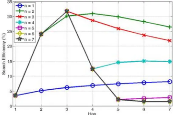
Fig. 4 illustrates that how the decision threshold n _{of DS would affect the system}

performance. Due to the page limit, we only show the result when p is set as 1. The case of n=1 _{is analogue to RW search}

with K _{equal to the number of the first}

Fig. 4. SE vs. hop count when p is set as 1 and

n is changed from 1 to 7. Power-law topology with N=10000. When n is set as 2, DS gets the best performance for almost all hop counts.

neighbor, which is about 3.55 in this case. Moreover, the case that n=7 _{is equal to}

the flooding search. As this figure shows, DS with n=7 _{sends the query messages}

aggressively in the first three hops and gets good SE_{. But the performance degrades}

rapidly as the hop increases. This is because that the cost grows exponentially with the path length between the query source and the target. On the contrary, SE

of RW is better than that of flooding when the hop is 5 to 7. When n _{is set as 2, DS}

gets the best SE _{for almost all hop counts.}

This figure shows that the choice of parameter n _{can help DS to takes}

advantage of different contexts under which each search algorithm performs well.

In order to obtain the best ( )n p,

combination, we illustrate the (n p SE, , ) results in Fig. 5. Here N _{is set as 10000,}

R _{is set as 0.01, and} TTL _{is set as 7.}

Under this context, when p is large (0.7 ~ 1), setting n=2 _{would get the best} SE_.

Moreover, the best n _{value increases as}

the p decreases, as Fig. 6 shows. For example, when p is set as 0.2, the best n

would be 6 or 7. This is because that when p is small, n _{should be increased}

to expand the coverage. On the contrary, when p is large, n _{should be decreased}

to limit the growth of query messages. Therefore, the parameters n _and p

provide the tradeoff between the search performance and the cost. It shows that the best SE _{is obtained when} ( )n p, _{is set}

as (2, 1). Due to the page limit, the best parameters for other contexts are skipped in this report, which can be found out through similar operation.

2.2.3.2 Search Time

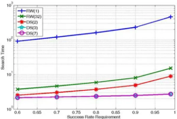
We show the numerical results of ST

in Fig. 7. In this case N _{is set as 10000,} R _{is set as 0.01, and} TTL _{is set as 7.}

Fig. 5. The effects of the parameters ( )n p, on the SE. Power-law topology with N=10000.

7

TTL= . The best SE is obtained when ( )n p,

is set as ( )2,1 .

Fig. 6. The best ( )n p, combination when

N is set as 10000, R is set as 0.01, and

TTL is set as 7.

Fig. 7. ST vs. SR requirement. R is set as 0.01 in this case. The number of walkers

K for RW are set as 1 and 32, respectively. The n of DS are set as 2, 3 and 7, and p is set as 1. TTL is set as 7 in this case, thus the DS with n = 7 is equal to flooding.

Similar results can be obtained when the parameters are set as other values. The numbers of walkers K _{for RW are set as 1}

and 32. The decision thresholds n _{are set}

as 2, 3 and 7, and p is set as 1. TTL _is

set as 7 in this case, thus DS with n=7 _is

equal to flooding. From Fig. 7 DS with large n _{always gets the short} ST _because

it always covers more vertices. On the contrary, RW with K=1 _{always gets the}

longest ST _{since its coverage is only}

incremental by one at each hop. When K

is set as 32, its coverage is enlarged and ST

can be improved. However, DS still performs better than RW with 32 walkers even when n _{is set as only 2. Note that}

when n _{is set as 3, DS performs as well as}

that with n=7_{, i.e., flooding, while does}

not generate as many query messages. In summary, DS with n=2 _and p=1 _would

get the best SE _{and significantly improve} ST _{in this case. While increasing} n _{to 3,}

although SE _{is a little degraded, the}

shortest ST _{is obtained.}

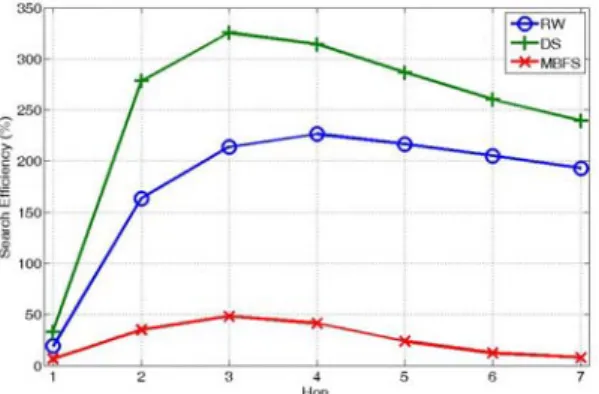
2.2.3.3 Performance of Knowledge-based Dynamic Search

The experimental results for different

search algorithms with knowledge building mechanism are shown in Fig. 8. With APS knowledge building mechanism, all search algorithms perform much better than they do without knowledge. Comparing these three search algorithms, for the case at

7

h= _, SE _{of DS is 24% better than that of}

RW, and 31 times better than that of MBFS. The outstanding performance results from the good tradeoff between the search performance and the cost.

2.2.3.4 Conclusion

In this project we propose DS algorithm which is a generalization of flooding, MBFS, and RW. DS algorithm overcomes the disadvantages of flooding and RW, and takes advantage of various contexts under which each search algorithm performs well. The operation of DS resembles flooding or MBFS for the short-term search, and RW for the long-term search.

We analyze the performance of DS based on some metrics including the success rate, search time, number of query hits, number of query messages, query efficiency, and search efficiency. Numerical results show that proper setting of the parameters of DS can obtain the short search time and provide a good tradeoff between the search performance and the cost. Under different contexts such as the number of peers in the network and the replication ratio of interested objects, the proposed DS algorithm always performs well. When combined with the knowledge-based search algorithms, the performance could be further improved.

Fig. 8. Performance comparison when combined with the knowledge-based search mechanisms. DS always performs the best.

2.3 子計畫三：兼顧服務品質與可重新組

態的下一代服務匯流網路架構

2.3.1 研究目標

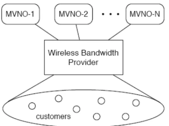
The concept of mobile virtual network operator (MVNO) arose during the planning and roll-out phase of 3G networks for the purpose of cost saving [18]. Sharing the wireless network has been analyzed to be a long-term beneficial strategy for the network operators [19]. There is a trend that network sharing will play an important role not only in the cellular but also in the broadband wireless access networks [20]. Therefore, we propose an architecture in which multiple MVNOs share the wireless bandwidth of a facility based operator called the Wireless Bandwidth Provider (WBP). By estimating the expected income from each MVNO, the WBP runs a dynamic programming algorithm to compute the optimal bandwidth allocations and achieve higher total revenue.

2.3.2 研究方法與步驟

In this section, we propose a generic model for multiple MVNOs to share the bandwidth of a single provider. In addition,

we also derive the formulas of the dynamic programming algorithm for the bandwidth provider to maximize its total revenue.

2.3.2.1 System Model

In our model (Fig. 10), there are N MVNOs and one wireless bandwidth provider (WBP). The WBP owns the core network and wireless access facilities such as 3G/3.5G base stations, WiMAX base stations, or Wi-Fi access points. It acts as a bridge between the customers and the MVNOs. The N MVNOs provide different sorts of services to the customers via the connection service of the WBP. The MVNOs are in charge of the service provisioning and customer management without operating a physical network.

The WBP charges for the connection service in a usage-based fashion. In order to maximize its total revenue, the WBP can adjust the bandwidth allocations to each MVNO every interval T. Changes of the allocations can only happen on time epochs

jT, j = 1, 2,…, and the setting should keep

unchanged in the following interval, which is denoted by Ij (see Fig. 11). The allocation decisions are based on the traffic patterns and the service contracts of the MVNOs. The traffic patterns of the customers can be supplied by the MVNOs or estimated by WBP according to previous measurements.

Fig. 10. A shared wireless data network model.

We assume that the customer arrival processes of the MVNOs are all Poisson but the arrival rates could change across different intervals. The arrival rates during

Ij are denoted by λj = [λj1, λj2,…, λjN]. The service time distributions are assumed general but do not change with time. Bi(t) denotes the CDF of the service time of MVNO-i and 1/μi is its average service time.

sj = [sj1, sj2,…, sjN] denotes the system state at the beginning of interval Ij and sji is the number of customers in MVNO-i at jT. The cost vector which WBP charges the MVNOs per customer per second can also vary across time intervals and is denoted by

cj = [cj1, cj1,…, cjN].

The bandwidth allocation during Ij is bj = [bj1, bj1,…, bjN] and the total bandwidth W of the WBP should not be exceeded, i.e.

1 ,

N ji

i= b ≤W ∀j

∑

bj at jT, it enforces new upper bounds to the number of customers of the MVNOs. This mechanism might incur some dropping of the customers. In compensation, the WBP should pay di to MVNO-i for each customer dropping event.

2.3.2.2 Estimate of the Income

According to the system model, we could model the behavior of each MVNO with an M/G/c/c queue with variable arrival rate. However, it is difficult to derive the transcient distribution of the number of customers in an M/G/c/c queue as the arrival rate changes. Therefore, in order to estimate the income of MVNO-i during interval Ij, we first derive the transcient

behavior of an M/G/∞ system. Afterwards, we truncate the probability mass function (PMF) of the M/G/∞ queue so that its maximum system size equals the capacity limit of the MVNO, and use the result as an approximate transcient distribution of the

M/G/c/c queue.

We assume that Xji(t) is the number of MVNO-i's customers who entered the system during (jT, jT+t] and are still in the system at jT+t, and Yji(t) is the number of MVNO-i's customers who were in the system at jT and remain in the system at

jT+t. Consequently, we have Xji (0) = 0 and

Yji (0) = sji. For t > 0, Xji(t) and Yji(t) are random variables. According to [21], it can be shown that the conditional probability of

Xji(t) = n given arrival rate λji, denoted as

fji(n,t; λji), would be

{

}

(

)

{

}

and the conditional probability of Yji(t) = n given Yji (0) = sji, denoted as gji(n, t; sji), is

{

}

(

)

[

]

_∫

r t =μq t . In fact, ri(t) is the residual

time distribution for the MVNO-i's

customers.

Let Zji(t) = Xji(t) + Yji(t) be the total number of customers of MVNO-i in system at time jT+t, and hji(n, t; sji, λji) denote the conditional probability that Zji(t) = n given

sji and λji. Hence,

{

}

∑

Note that the equation above is derived under the assumption that the system size can grow without bound. Assume that the bandwidth allocated to MVNO-i is only bji during the j-th interval and the corresponding maximum number of customers is vi(bji). We must truncate the PMF to approximate the distribution of the system size in the M/G/c/c queue. As a result, the probability that Zji(t) = n given sji, λji, and bji, denoted as yji(n, t; sji, λji, bji), can be approximated as

{

}

∑

The expected total usage of MVNO-i's customers during Ij, denoted as Uji, given the initial system size sji, the arrival rate λji and the bandwidth limit bji should be

0

( , , ) T ( ) , ,

ji ji ji ji ji ji ji ji

U s λ b =

∫

However, there is no closed form formula to carry out this integration. We compute the income estimation numerically with the following equation instead.

1 ( ) 1 1 ( , ) ( ) , , ( , ; , ) i ji K ji ji ji ji ji ji ji ji ji k v b K ji ji ji ji ji k n G s b c E Z t s b c n y n k s b λ τ λ τ τ λ = = = ⎡ ⎤ = _{⎣ ⎦} = ⋅

∑

∑ ∑

, where τ = T/K, and K is an integer. The value of τ affects both the estimation

accuracy and the amount of computation required. There is a trade-off in choosing the value. If τ is too small, it will lead to higher computation complexity. On the opposite, if τ is too large, there will be accuracy issues.

2.3.2.3 The Optimality Equation

Maximizing the total returns in the previously described model is a positive dynamic programming problem [22]. According to the derivation in the previous subsection, the expected total return from all MVNOs during interval Ij given the state

sj, the arrival rate λj, and the bandwidth allocation bj (i.e. the action taken) can be expressed as 1 1 ( , , ) ( , , ) ( , ) ( , , ) ( , ) ( , ) ( ) j j j j j j j j j j j N j j j j ji ji ji ji i N j j j i ji i ji i R G L G G s b L d s v b λ = + = = − = ⎡ ⎤ = _⎣ − _⎦

∑

∑

The operation [x]+ equals x if x>0 and 0 otherwise. We can also obtain the transition probability from state sj to sj+1 as

{

}

∏

Thus, the optimality equation is

1 1 1 1 1 ( , ) max ( , , ) ( , ) ( , ) j j j j j j j j j j j j j j V R P V + + + + + ⎧ ⎫ ⎪ ⎪ = ⎨ + ⎬ ⎪ ⎪ ⎩ ∑ ⎭ b s s λ s λ b s s s λ

and the optimal policy bj* is the bandwidth allocation which makes Vj(sj, λj) maximal.

Let Mi denote the maximum number of customers of MVNO-i when the highest level of bandwidth is allocated to it. The size of the state space is approximately

1

( _iN _i)

O

∏

(

)

∏

∑

the number of possible bandwidth allocations.

Note that one can incorporate as many stages of recursion as possible when computing the optimal allocation. However, the solution would converge after extending to certain number of stages. Since the computing process of the DPA is actually backward, it is important to decide the number of stages in advance to avoid the waste of computing power. There are more discussions on this issue in next subsection.

2.3.3 結果與討論

2.3.3.1 Simulation Environment

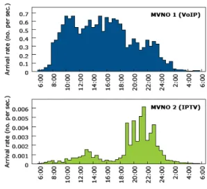
We evaluate the effectiveness of the proposed DPA with C++ coded simulations. There are two MVNOs in the simulated scenario. MVNO-1 is a VoIP operator and MVNO-2 is an IPTV operator. We also assume the WBP operates a WiMAX based

wireless access network.

The total MAC layer bandwidths provided by one single BS are set to be 9Mbps and 6Mbps for downlink and uplink respectively. According to [23], these amounts of bandwidth can be achieved via either a 5 or 10 MHz channel if efficient modulation and coding schemes are adopted.

We assume that the VoIP system adopts the G.711 codec and thus each direction of a voice call requires 80Kbps of bandwidth at MAC layer. The distribution of the call duration is exponential with mean = 100 seconds. The bandwidth requirement for a downlink IPTV stream is assumed to be 768Kbps and the service time distribution is exponential with mean = 2500 seconds.

Fig. 12 shows the arrival rate patterns for a 24-hour period and Table II gives the costs and the dropping penalties of each MVNO. The pricing policy together with the traffic pattern affects the expected revenue from each MVNO and thus the allocation strategy of the WBP. Therefore, it

Table II. Usage-based prices per customer per second.

MVNO-1(VoIP) MVNO-2(IPTV) regular discount regular discount Time period 8:00 ~ 23:00 23:00 ~ 8:00 18:00 ~ 24:00 24:00 ~ 18:00 Usage cost 0.005 0.0015 0.07 0.035 Drop penalty 25.0 40.0

Fig. 12. Arrival patterns adopted in the simulation.

is possible that an MVNO can demand more bandwidth by accepting higher costs. However, we adopt only fixed pricing policy in this paper in order to put more emphasis on the performance of DPA. The usage costs and drop penalties should be negotiated by the WBP and the MVNOs in the beginning. Further research of the dynamic pricing mechanisms will be our future work.

The bandwidth allocation takes 1Mbps as the basic unit and the minimum allocated bandwidth for both MVNOs is also set to be 1Mbps. However, because of the bandwidth asymmetry, the upper bound of the number of VoIP customers is determined by the uplink bandwidth. Thus, the maximum bandwidth for MVNO-1 is 6Mbps. The computation of the DPA for each possible system state should be completed before the start of each interval. Then the WBP decides which bandwidth allocation (action) to take according to the actual system state at the start of the interval and the computed results.

Based on these parameter settings, maximum number of customers of the two MVNOs are 75 and 10 respectively, and the size of the state space is 508. The number of

possible bandwidth allocations (Cb) is 6. During simulation, the length of each interval T is set to be 30 minutes, i.e. the WBP runs DPA and decides the optimal action every 30 minutes. The value of τ is set to be 10 seconds, i.e. K = 180. The number of dynamic programming stages affects both the effectiveness and the amount of computations of the proposed algorithm. We ran simulations for 1 to 5 stages and compare the results with the fixed bandwidth allocation scenario (in which 4.5Mbps allocated for both MVNO-1 and MVNO-2).

We ran 20 repetitions of the simulations, each lasting for a 24-hour period, and took the average of the results.

2.3.3.2 Simulation Results

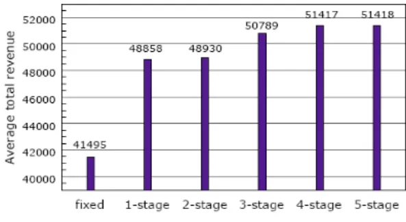
Fig. 13 compares the total revenues achieved by adopting the fixed allocation scheme or DPA with different number of stages. The improvements of the DPA are around 14.5% to 20.5%. As the number of

Fig. 13. Comparison of the average total revenues obtained under different stages of dynamic

programming, using default parameters.

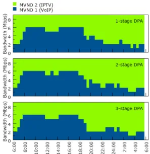
Fig. 14. Bandwidth allocation decisions generated by 1, 2 and 3-stage DPA.

stages increases, the gain of the total revenue gradually saturates just as expected.

Fig. 14 gives an example of the resulting bandwidth allocations via computing different number of stages in DPA. We find that the results of 4 and 5-stage DPA are very close to the 3-stage DPA in most simulation repetitions under the default parameter settings. Hence, only the plots of 1 to 3-stage DPA bandwidth allocations are shown in Fig. 14. This example shows that one can get “smoother'” bandwidth allocations, i.e. there are less bandwidth fluctuations, if more stages are incorporated in the DPA. In addition, since the average service time of IPTV customers is longer than the length of a single stage, DPA with 3 or more stages can predict the behavior of them well and allocate more resources to MVNO-2. On the other hand, the results in the first two plots do not allocate as sufficient bandwidth to MVNO-2 during the peak of its arrival pattern.

The blocking probabilities under different stages of DPA are shown in Table III. Obviously, all DPA results outperform the fixed allocation scheme. As the number of stages increases, the blocking probabilities of IPTV customers decrease while those of the VoIP customers increase. This is because the optimality equation considers only the total revenue. It is

possible to add some QoS constraints, such as the minimum blocking probability, in the service level agreements between WBP and MVNOs, and thus the optimality equations should be revised to reflect the change in the model.

In order to examine the relationship between the number of stages and the average service time, we ran another set of simulations with the average connection duration of the IPTV customer doubled (i.e. mean = 5000 sec.). Accordingly, the arrival rates are halved to maintain the same traffic loads. Fig. 15 is the resulting average total revenues. Notice that the total revenues are higher while the traffic loads are kept the same. This is because that the blocking rate of IPTV customers decreases as the arrival rate gets smaller. Therefore, the increase in revenue mainly comes from MVNO-2.

The revenue improvements vary from 17.7% to 23.9% in the second set of simulations. Furthermore, unlike the previous case, the improvement of total revenue saturates after incorporating 4 stages instead of 3 stages. It shows that more stages are required if the probability that a connection duration might span several stages increases. However, the

Table III. Blocking probabilities with default parameters.

fixed 1-stage 2-stage 3-stage 4-stage 5-stage MVNO-1 0.086 0.037 0.057 0.069 0.071 0.071 MVNO-2 0.343 0.230 0.198 0.170 0.169 0.168

Fig. 15. Comparison of the average total revenue results with doubled IPTV customer service time

number of stages required to attain saturation not only depends on the average service time but also the service time distribution. It is yet to be shown either via mathematical derivation or more extensive simulations.

Last but not least, using a Xeon 2.8GHz CPU with 1GB RAM, the execution time of the DPA is found to require only about 42 seconds per stage, which implies that such approach can be employed in real operations.

2.2.3.3 Conclusion

We proposed a dynamic programming algorithm together with the estimation formulas of the system behavior to determine the optimized bandwidth allocations for the wireless bandwidth provider. According to the simulation results, we have found that by computing the optimal allocation considering both the possible income and loss across several stages, DPA can achieve quite significant improvements in the average total revenue.

In future work, spectrum trading mechanisms will be incorporated in the multi-cell spectrum sharing model and the algorithms will be evaluated by simulations. For the bandwidth sharing model, auction based dynamic pricing of the bandwidth and therefore the strategies of the MVNOs can be further incorporated. In addition, it is also possible that more than one WBPs coexist in the same area, and the competition among different WBPs can introduce high complexity in deciding the strategies in this market. It should be easy

to develop other models and various resource allocation algorithms based on the works presented in this report.

2.4 子計畫四：分散式視訊偵搜所需整合 性網路與計算服務之研究 2.4.1 研究目標 本子計畫之研究工作為探討 IP 網路 上以 P2P 社群進行視訊偵搜服務與與資 訊分享的商務模型。主要包括以下兩部分: (一) 有影像品質保證的移動視訊偵捜路 由演算法之研究與系統實做，(二) P2P 社 群使用者行為模型的建立與分享誘因實 驗設計。 前者之研究目的是在隨意網路上實 現 有 影 像 品 質 保 證 的 移 動 視 訊 偵 搜 服 務。如要在隨意網路上實現偵搜服務，由 於隨意網路裡的節點(node)都是可以自由 移動的，導致每一個節點傳輸範圍內的鄰 居也會隨時間而不同，因此必須要取得位 置資訊，並且移動而動態(dynamically)調 整傳輸的路徑。再者，802.11 架構設計使 得多次跳躍(Multi-Hop)的傳輸和傳輸距 離越遠(Fig. 16)，會對視訊傳輸之品質造 成越嚴重影響。因此我們研究以下兩個課 題：1.如何週期性取得網路上其他節點的 資訊、2. 如何建立並動態調整跳躍數少、 能提供足夠的資料傳輸速度傳輸路徑。 使用者行為模型的實證分析與實驗 設計之主要目的則為提出架構處方性模 型之方式以進行誘因設計，提高社群內分 享資源數量與品質。 Fig. 17. 鄰居資訊路由法協定堆疊

2.4.2 研究方法與步驟 2.4.2.1 有影像品質保證的移動視訊偵捜 路由演算法之研究與路由演算法實做 我們首先利用實驗了解隨意網路傳 輸特性後，在 IP 層設計了一個鄰居資訊 表路由法協定(Fig. 17)，包含鄰居資訊列 表交換堆疊 - NIL exchange stack - 和鄰 居資訊路由演算法 - NILRA，來解決所提 出的兩個主要研究問題。其中NIL 交換協 定 可 以 透 過 各 節 點 週 期 性 相 互 廣 播 (broadcast)來保持各節點傳輸範圍內的最 新鄰居資訊，包含IP 位址，經緯度位置， 移動速度，方向和資料傳輸率。而路由演 算法(NILRA)的主要想法(Fig. 18)是接收 到搜尋封包的node，如果自身與目的地之 間的距離不在門檻值內，則在自身的鄰居 列表裡，尋找符合傳輸速度條件的鄰居中 位置最靠近目的地的 node(利用經緯度位 置和Data rate 資訊)，接者將搜尋封包送 給此node，如此類推即可尋找到一條跳躍 (HOP)數少且符合傳輸速度的路徑。而建 立好的路徑上之節點也可以利用移動速 度與方向這兩個資訊來保持路徑完整。 實做方面，我們在802.11 架構下以 4 台的筆記型電腦組成隨意網路，在應用層 上運用visual basic .NET 與 SQL2000 來實 做NIL 交換堆疊(NIL exchange stack)，以 此堆疊設計來動態的建立與更新鄰居資 訊列表。而 NILRA 實做則使用 visual basic .NET 設計路由演算法程式，來自動 的執行路徑搜尋。最後與最短路徑法比較 影像傳輸品質，證明此路由法的確可找到 有影像品質保證的路徑(Table IV)。 2.4.2.2 P2P 社群使用者行為模型的建立 與分享誘因實驗設計 本研究探討了包含四項行為：網路社 群的加入、離開及社群服務的使用、提 供。研究議題分為兩項：(1) 無誘因制度 下，建構以網路社群經驗資料為基礎之使 用者集體行(collective behavior)模型，(2) 固定社群分享資源下，為架構使用者對獎 酬制度反應模型之實驗設計。為架構使用 者集體行為模型，我們基於過去設計之使 用者行為模型，並在無誘因制度的前提 下，利用網路社群的實證資料探討行為機 率與網站資源的關係，並進行迴歸分析， 驗證其模型正確性，並以曲線配適法導出

Fig. 18. node 處理搜尋封包(RREQ)的邏輯步驟

TCP Throughput 0 1 2 3 4 5 6 1 2 3 4 HOP數 T hr oughput (M bps ) TCP Throughput Fig. 16. HOP 數與吞吐量(實驗數據) 數據資料 路由方法 路徑吞吐量 資料遺失率 人眼評分 NILRA 之路徑 1.803Mbps 趨近0 5 分 最短路徑法 之路徑 0.852Mbps 8.13% 2 分 Table IV. 路由法之數據結果比較(實驗結果)

其模型參數，成果如 Fig. 19 所示。另外 為架構使用者對獎酬制度反應模型之實 驗設計，我們以相較分等(relative ranking) 的獎酬制度，在固定社群資源下，設計二 因子實驗設計，探討在不同獎酬制度中， 使用者行為的反應模型。藉由上述使用者 行為模型的實證分析與實驗設計，為未來 社群管理者提供建立架構處方性模型之 方式以進行誘因設計。 三、參考文獻

[1] IEEE Std 802.16-2004, IEEE standard for local and metropolitan area networks part 16: air interface for fixed broadband wireless access systems, 2004.

[2] T. Kim, H. Lim, J. C. Hou, “Improving Spatial Reuse through Tuning Transmit Power, Carrier Sense Threshold, and Data Rate in Multihop Wireless Network”, MobiCom’06, 2006.

[3] H. Viswanathan, S. Mukherjee, “Throughput-Range Tradeoff of Wireless Mesh Backhaul Networks”, IEEE JOURNAL

ON SELECTED AREAS IN COMMUNICATIONS, VOL. 24, NO. 3, March

2006.

[4] G. Brar, D. M. Blough, P. Santi,

“Computationally Efficient Scheduling with the Physical Interference Model for Throughput Improvement in Wireless Mesh Networks”, MobiCom’06, 2006

[5] A. Basu, B. Boshes, S. Mukherjee, S. Ramanathan, “Network Deformation: Traffic-Aware Algorithms for Dynamically Reducing End-to-end Delay in Multi-hop Wireless Networks,” MobiCom’04, 2004. [6] T. S. Rapport, Wireless Communications

Principles and Practice, Prentice Hall, 1998.

[7] D. Milojicic, V. Kalogeraki, R. Lukose, K. Nagaraja, J. Pruyne, B. Richard, S. Rollins, and Z. Xu, “Peer-to-Peer Computing,” Tech. Rep. HPL-2002-57, HP, 2002.

[8] D. Stutzbach, R. Rejaie, N. Duffield, S. Sen, W. Willinger, “Sampling Techniques for Large, Dynamic Graphs,” Global Internet Symposium, April 2006.

[9] A. H. Rasti, D. Stutzbach, R. Rejaie, “On the Long-term Evolution of the Two-Tier Gnutella Overlay,” Global Internet Symposium, April 2006.

[10] K. Sripanidkulchai, “The popularity of Gnutella Queries and its Implications on Scalability,” white paper, Carnegie Mellon Univ. Pittsburgh, Feb. 2001.

[11] M. Jovanovic, F.Annexstein, and K. Berman, “Scalability Issues in Large Peer-to-Peer Networks: A Case Study of Gnutella,” Tech. Report. Univ. of Cincinnati, Lab. For Networks and Applied Graph Theory, 2001. [12] B. Yang and H. Garcia-Molina, “Improving

search in peer-to-peer networks,” in Proceedings of the 22nd International Conference on Distributed Computing Fig. 19. 使用者行為模型分析結果

Systems (ICDCS’02). Vienna, Austria: IEEE Computer Society, pp. 5–14, July 2002. [13] M. E. J. Newman, S. H. Strogatz, and D. J.

Watts. “Random graphs with arbitrary degree distribution and their applications,” Phys. Rev. E 64, 026118, 2001.

[14] H. Wang, T. Lin, “On efficiency in searching networks,” in Proceedings of IEEE INFOCOM, pp. 1490-1501, 2005.

[15] Z. Ge, D. R. Figueiredo, S. Jaiswal, J. Kurose, and D. Towsley, “Modeling Peer-Peer File Sharing Systems,” in Proceedings of IEEE INFOCOM, pp. 2188-2198, 2003.

[16] S. Saroiu, P. K. Gummadi, S. D. Gribble, “A Measurement Study of Peer-to-Peer File Sharing Systems,” MMCN, San Jose, CA, USA, January 2002.

[17] J. Chu, K. Labonte, and B. Levine, ”Availability and Locality Measurements of Peer-to-Peer File Systems,” in ITCom: Scalability and Traffic Control in IP Networks. July 2002, vol. 4868 of Proceedings of SPIE.

[18] G. Beckman and G. Smith, “Shared networks:

making wireless communication affordable,”

IEEE Wireless Communications, vol. 12, no. 2,

pp. 78-85, April 2005.

[19] A. Bartlett and N. N. Jackson, “Network planning considerations for network sharing in UMTS,” in Proc. IEEE Third International

Conference on 3G Mobile Communication Technologies, May 2002, pp. 17-21.

[20] B. T. Olsen, D. Katsianis, D. Varoutas, K. Stordahl, J. Harno, N. K. Elnegaard, I. Welling, f. Loizillon, T. Monath, and P. Cadro, “Technoeconomic evaluation of the major telecommunication investment options for European players,” IEEE Network, vol. 20, no. 4, pp. 6-15, July/August 2006.

[21] D. Gross and C. M. Harris, Fundamentals of

Queueing Theory, 3rd _{ed. John Wiley & Sons,}

Inc., 1998.

[22] S. Ross, Introduction to Stochastic Dynamic

Programming. Academic Press, Inc., 1983.

[23] WiMAX Forum, “Mobile WiMAX – Part I: A Technical Overview and Performance Evaluation,” August 2006.