以區域為基礎利用小波轉換和形態學運算的影像擷取

全文

(1)國立交通大學資訊科學系碩士論文. 以區域為基礎利用小波轉換和形態學運算的影像擷取 Region-Based Image Retrieval Using Wavelet Transform and Morphological Operation. 研究生：莊逢軒指導教授：薛元澤. 教授. 中華民國九十四年六月.

(2) 以區域為基礎利用小波轉換和形態學運算的影像擷取. 學生：莊逢軒. 指導教授：薛元澤. 國立交通大學資訊科學學系﹙研究所﹚碩士班. 摘要. 近年來，隨著電腦科技發展迅速和生活數位化，數位影像資料庫的數量和容量正以極快的速度增加。如何有效的管理一個大型的數位影像資料庫也越來越重要。因此影像檢索便成為一個重要的研究領域。以區域為基礎的影像檢索法已經被證明比影像內容為基礎的影像檢索法來的有效率，因為它利用物件來描述影像而非使用整張影像內容。本研究所提出的方法先利用 K-means 分群法將影像切割成數各區域，並分別使用小波能量和形態學運算來描述區域的紋理、彩色和形狀特徵。再依此計算查詢影像和資料庫中影像的相似度，並選出最相近的影像。實驗結果顯示我們所提出的方法是快速且有強韌性的。. i.

(3) Region-Based Image Retrieval Using Wavelet Transform and Morphological Operation. student：Feng-Hsuan Chuang. Advisors：Dr.Yuang-cheh Hsueh. Institute of Computer and Information Science National Chiao Tung University ABSTRACT. In recent year, with the rapid development of computer technology and digitize life, digital image databases have grown enormously in both size and number. How to effectively manage the large image databases is more and more important. So image retrieval has become an important research topic. Region-based image retrieval has been proven more effective than content-based image retrieval, because it overcome the deficiencies of content-based image retrieval by representing images at the object-level. The method proposed in this thesis utilizes the K-means clustering algorithm to segment the image into regions, and use the wavelet energy and morphological operator to extract texture, color and shape features to describe regions, respectively. Then we can retrieve the most similar images according the similarity between query image and database image. Experimental results indicate the proposed method is fast and robust.. ii.

(4) 誌謝. 我在這裡要感謝我的指導教授薛元澤教授，兩年來對我孜孜不倦的教誨，教導我研究學問的方法及待人處世道理，讓我畢生受益無窮，以及我的口試委員張隆紋教授與陳玲慧教授，二位老師不吝指教，讓這篇論文更加完善。我還要感謝吳昭賢學長，給予我論文研究及寫作方面等的各種建議，感謝何昌憲同學、王蕙綾同學、高薇婷同學、蔡盛同同學在這兩年內與我共同努力，互相砥礪。另外，我要感謝呂盈賢學弟、江仲庭學弟、林明志學弟、劉裕泉學弟、顏佩君學妹及王慧縈學妹陪我度過這段快樂的實驗室生活。僅將此論文獻給我親愛的的家人與朋友，我的父母及妹妹，感謝他們在這段期間給我的關心、支持與鼓勵，祝福他們永遠健康快樂。. iii.

(5) CONTENTS ABSTRACT (CHINESE)............................................................................................................i ABSTRACT (ENGLISH)...........................................................................................................ii ACKNOWLEDGEMENT.........................................................................................................iii CONTENTS ..............................................................................................................................iv LIST OF FIGURES ..................................................................................................................vii LIST OF TABLES ....................................................................................................................vii. CHAPTER. 1 ..........................................................................................................................1. 1.1 Motivation ....................................................................................................................1 1.2 Backgrounds .................................................................................................................2 1.2.1 Overview of Content-Based Image Retrieval....................................................2 1.2.2 Overview of Region-Based Image Retrieval.....................................................3 1.3 Thesis Organization...................................................................................................... 6 CHAPTER. 2 ..........................................................................................................................7. 2.1 Review of Image Retrieval ...........................................................................................7 2.1.1 Color Spaces ......................................................................................................7 2.1.1.1 RGB Color Space ...................................................................................7 2.1.1.2 HSV Color Space....................................................................................8 2.1.1.3 YUV and YIQ Color Space ....................................................................9 2.1.1.4 Luv color space.....................................................................................10 2.1.2 The Feature of Color Image.............................................................................10 2.1.2.1 Color Histogram ...................................................................................10 2.1.2.2 Color Moments ..................................................................................... 11 2.1.2.3 Texture ..................................................................................................12 2.1.3 Region-Based Image Retrieval........................................................................14 iv.

(6) 2.1.3.1 IRM：Integrated Region Matching for Image Retrieval .....................14 2.1.3.2 Research Issue ......................................................................................16 2.2 Wavelet Transform and Multiresolution Processing ..................................................17 2.2.1 Image Pyramid.................................................................................................18 2.2.2 Discrete Wavelet Transform............................................................................19 2.3 Mathematical Morphology .........................................................................................21 2.3.1 Basic definition................................................................................................22 2.3.2 Morphological operations................................................................................23 2.3.3 Extension to Gray-Scale images......................................................................24 2.3.4 Morphological Gradient ..................................................................................26 CHAPTER. 3 ........................................................................................................................28. 3.1 Overview of Our Image Retrieval System .................................................................28 3.2 Image Segmentation ...................................................................................................29 3.2.1 K-means Clustering Algorithm and Cluster Number ......................................29 3.2.2 Color Image Segmentation by K-means Algorithm ........................................32 3.3 Feature Extraction of Region......................................................................................33 3.3.1 Texture Feature ................................................................................................34 3.3.2 Color Feature ...................................................................................................35 3.3.3 Region Feature Vector .....................................................................................36 3.4 Similarity Measure .....................................................................................................36 CHAPTER. 4 ........................................................................................................................39. 4.1 Experiment Environment............................................................................................39 4.2 The First Experiment ..................................................................................................40 4.3 The Second Experiment .............................................................................................43 4.4 The Third Experiment ................................................................................................46 4.5 Relevance Feedback ...................................................................................................47 v.

(7) CHAPTER. 5 ........................................................................................................................51. 5.1 Conclusions ................................................................................................................51 5.2 Future Works ..............................................................................................................52 Reference ..................................................................................................................................53. vi.

(8) LIST OF FIGURES Fig. 1-1. Overview of image retrieval techniques ............................................................4. Fig. 1-2. The architecture of region-based image retrieval ..............................................5. Fig. 2-1. RGB color space and the color cube..................................................................8. Fig. 2-2. HSV cone. ..........................................................................................................9. Fig. 2-3. Two different images with similar color histograms ....................................... 11. Fig. 2-4. Integrated region matching. .............................................................................15. Fig. 2-5. A pyramidal image structure............................................................................18. Fig. 2-6. System block diagram for creating an image pyramid. ...................................19. Fig. 2-7. Two-dimensional four-band filter band. ..........................................................20. Fig. 2-8. The illustration for the wavelet decomposition (a) Decomposition process of wavelet transform; (b) Pyramidal structure of wavelet decomposition .......21. Fig. 2-9. Examples of structuring elements....................................................................22. Fig. 2-10. Example of (a) Transaction and (b) Reflection................................................22. Fig. 2-11. (a) Set A; (b) Structuring element B; (c) The Dilation of A by B; (d) The Erosion of A by B; (e) The Closing of A by B; (f) The Opening of A by B .....24. Fig. 2-12. (a) The original of Lena image; (b) Dilation of Lena image; (c)Erosion of Lena image .......................................................................................................25. Fig. 2-13. (a) The original of Lena image; (b) Closing of Lena image; (c) Opening of Lena image .......................................................................................................26. Fig. 2-14. (a) The original of Lena image; (b) Morphological gradient of Lena image...27. Fig. 3-1. Overview of Our Image Retrieval System.......................................................29. Fig. 3-2. The process of image segmentation. (a) Original image; (b) Clustering algorithm applied in the LL subband; (c) Final segmentation result................30. Fig. 3-3. Example of segmentation results. (a) Original image; (b) Segment with wi =1, i=1,…9; (c) Segment with w1 =1; wi = 4, i=2,…,9 ........................32 vii.

(9) Fig. 3-4. Another example of segmentation results. (a) Original image; (b) Segment with wi =1, i=1,…9; (c) Segment with w1 =1; wi = 4, i=2,…,9......................33. Fig. 3-5. The illustration for the generation of hierarchical region feature vector. (a) One region in an image; (b) Spatial orientation tree; (c) Corresponding regions in wavelet domain................................................................................34. Fig. 3-6. The illustration of overall image similarity measure .......................................38. Fig. 4-1. The examples of the image database. ..............................................................39. Fig. 4-2. The example of emphasize I and Q component in texture feature. (a) The retrieval result of wY, wI and wQ are the same weight value; (b) The retrieval result of set higher weight value to wI and wQ more than wY. ............41. Fig. 4-3. Another example of emphasize I and Q component in texture feature. (a) The retrieval result of wY, wI and wQ are the same weight value; (b) The retrieval result of set higher weight value to wI and wQ more than wY .............42. Fig. 4-4. The precision-recall curve. (a) The result of category 1; (b) The result of category 3; (c) Compare category 1 with category 3........................................45. Fig. 4-5. Robust test of our image retrieval system. (a) The retrieval result of add noise; (b) The retrieval result of shift; (c) The retrieval result of mirror; (d) The retrieval result of flip. ..........................................................................47. Fig. 4-6. The example of relevance feedback. (a) The first retrieval result; (b) After adjusting weights, the second retrieval result...................................................49. viii.

(10) LIST OF TABLES Table 4-1. The precision of our image retrieval system using different features ...............43. ix.

(11) CHAPTER. 1. Introduction. 1.1 Motivation In recent year, with the rapid development of computer technology and digital life, the demand of multimedia services becomes more and more important. Thus, how to fast and effectively search similar images among large databases is a very important issue. So image retrieval has become an important research topic. Image retrieval is defined as the retrieval of relevant images from an image database based on automatically derived imagery features [1]. The need for efficient image retrieval has increased tremendously in many application areas such as medical, crime prevention, trademark, education, and web image classification and searching. The images used in different application aspects have different properties. The MPEG-7 Visual Description Tools consist of descriptors that cover the following basic visual features: color, texture, shape, motion, localization, and face recognition [18]. For example, when we retrieve a texture image, we should emphasize texture features more than other features in order to get higher precision rate. Therefore, we should select the proper features of image database to design the retrieval method. In this thesis, we construct a region-based image retrieval system to retrieve natural images. First, we will segment each image in image database into regions, and utilize the wavelet energy and morphological operator to extract texture, color and shape features to describe regions, respectively. Then the system will store these features to form the feature database. A user will choose a query image from the image database to start the retrieval procedure to find matching images. Then the system will automatically compute the similarity value by comparing the features of query image with all features in the feature database. At 1.

(12) last, the system will sort the images in descending order according to similarity values and present retrieval results.. 1.2 Backgrounds In this section, we will introduce the content-based image retrieval in section 1.2.1. Then in section 1.2.2, we will introduce the region-based image retrieval that is the extension of content-based image retrieval.. 1.2.1 Overview of Content-Based Image Retrieval Content-based image retrieval (CBIR) utilizes the image visual contents to extract the global low-level features to describe the whole image. First, all images in image database will be extracted the low-level features, which are their descriptors. The user will supply a query image to start the retrieval procedure, this mode is called Query-by-Example (QbE). Then, relevant images are retrieved by comparing the low-level features of the query image with features of each image in the image database. Because the CBIR system extracts the global low-level features, such as histogram and moment, thus the information about object location, shape, and texture is discarded. Moreover, it is sensitive to intensity variation, and color distortion [1]. QBIC (Query by image content) [2], [3] developed by IBM Almaden Research Center is one of the earliest content-based image retrieval systems. QBIC system uses color, texture, shape, and sketch as the indexes of each image inside the database. Users may pose queries in three ways. The first way is to find similar images by specifying a major color to represent the desired images. The second method uses a color histogram to represent the approximate color percentage of the desired images. The third method is that a user specifies a query by sketching a color layout. QBIC emphasizes the distribution of the pixels and the difference between the colors of the pixels, but it is not concerned with the objects and the relationship 2.

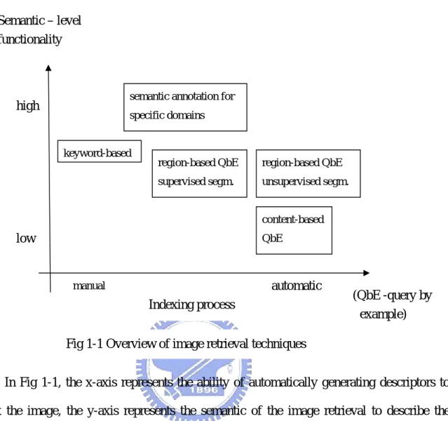
(13) of objects. Thus, this system is suitable for nature images. In addition, although QBIC provides these three features, users can choose only one kind of features to do retrieval, so how to combine various features to get better results is a significant research topic. MARS (Multimedia Analysis and Retrieval System) [4] was developed by University of Illinois at Urbana-Champaign. The goal of the MARS is to design and develop an integrated multimedia information retrieval and database management infrastructure. MARS/IRS is an image retrieval system which support similarity and content-based retrieval of images based on a combination of their color, texture, shape, and layout properties. Furthermore, MARS/IRS utilizes extracted features to generate texture annotations which describe the salient textural properties of images. Thus, an user can combine image properties and text annotation in specifying queries. MARS proposes an relevance feedback architecture in image retrieval and integrates query vector refinement, automatic matching tool selection, and automatic feature adaption. Other famous systems like CMU Informedia [5], Columbia VisualSEEK [6], and Stanford WBIIS [7] are also belonging to CBIR system.. 1.2.2 Overview of Region-Based Image Retrieval Region-based image retrieval (RBIR) is the extension of content-based image retrieval. It overcomes the deficiencies of CBIR by representing images at the object-level. Because the CBIR extracts the global features to describe images, thus the information about object location, shape, and texture is discarded. Furthermore, using the features of regions to describe objects are more semantic than using the global features. The object-level representation is intended to be close to the perception of the human visual system [1]. In [8], V. Mezaris and M.G. Strintzis indicate that to describe images, RBIR is more semantically than CBIR. Here, we use Fig 1-1 [8] to describe evolution of image retrieval techniques.. 3.

(14) Semantic – level functionality. semantic annotation for. high. specific domains. keyword-based. region-based QbE. region-based QbE. supervised segm.. unsupervised segm.. content-based. low. QbE. automatic. manual. Indexing process. (QbE -query by example). Fig 1-1 Overview of image retrieval techniques In Fig 1-1, the x-axis represents the ability of automatically generating descriptors to index the image, the y-axis represents the semantic of the image retrieval to describe the image. The keyword-based approach is the first attempt for image retrieval. It is based on exploiting existing image captions to classify images in predetermined classes or in a restricted vocabulary [9]. By employing the predetermined classes or textual annotations that is generated manually, this approach can describe the image more semantically. But this approach has several restricted and inconvenience, such as query the undefined image in a restricted vocabulary, manually generated the textual annotation and new added annotation to the vocabulary. Similarly, semantic annotation approach also relies on predetermined or manually added textural annotation. But in well-structured specific domain applications (e.g sports and news broadcasting), domain-specific features that facilitate the modeling of higher level semantics can be extracted [10], [11].. 4.

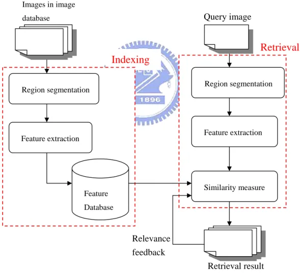
(15) To overcome the limitations of the keyword-based approach, using the image visual content being the indexing has been proposed (CBIR). Although the CBIR can automatically generated descriptor to describe images, but the extracted global low-level features cannot perfectly express the high-level semantics that human are familiar with. Hence, the concept of object-level representation is proposed. Recently, the Berkeley’s Blobword [12] which belong to the RBIR system, demonstrate the improvement of retrieval result attained by using region-based. indexing. features. rather. than. global. image. features,. under. the. Query-by-Example scheme [8]. In Fig 1-2, we show the architecture of the RBIR.. Images in image. Query image. database. Retrieval Indexing Region segmentation. Region segmentation. Feature extraction. Feature extraction. Similarity measure. Feature Database. Relevance feedback Retrieval result Fig 1-2 The architecture of region-based image retrieval. In Fig1-2, this architecture consists of indexing part and retrieval part. The indexing part will decompose each image in image database into regions, and extract the features to describe 5.

(16) regions. The system will store all features to form the feature database for retrieval usage. In retrieval part, user will provide a query image to start the retrieval procedure. Similarly, the same operation will segment the query image, and extract the feature to describe the regions. At the similarity measure stage, the system will evaluate the similarity value according to the comparing result of the feature of query image with each feature in the feature database and present the retrieval result. There are some famous RBIR systems, such as Stanford SIMPLIcity [13], and UCSB NeTra [14].. 1.3 Thesis Organization The remainder of this thesis is organized as follows. In chapter 2, we will survey the research of region-based image retrieval and discuss some issues need to concern. Then, we will survey the concept of wavelet transform and morphological operations. In chapter 3, we will present our method include using the K-means algorithm to segment an image into regions and extract features to describe regions. Then, we will define how to evaluate similarity value between two images. In chapter 4, we will experiment with different features and robust test. Then, we will compare the performance of our method with other method. Finally, we implement the relevance feedback algorithm proposed by Shin [35] to get more similar retrieval result. In chapter 5, the conclusion and future work will be stated.. 6.

(17) CHAPTER 2 Previous Research In this chapter, we will describe several related researches about color image retrieval in section 2.1. In section 2.2, the concept of the wavelet transform will be introduced. Basic morphological operators will be described in section 2.3.. 2.1 Review of Image Retrieval In this section, we will describe some color spaces in 2.1.1. In section 2.1.2, we will describe some frequently used features in image retrieval. Then in section 2.1.3, we will introduce some existing region-based image retrieval systems.. 2.1.1 Color Spaces The perception of color is very important for humans. Humans use color information to distinguish objects, materials, foods, and places…etc. Since human visual system has three types of color photoreceptor cone cells, three components are required to describe a color sufficiently. Thus, a color is commonly represented as a point in a three-dimensional color space such as RGB, HSV, YIQ, and YUV color spaces.. 2.1.1.1 RGB Color Space The RGB color space is based on a Cartesian coordinate system. The RGB color space represents colors in terms of Red、Green and Blue coordinates. The RGB color space and color cube is shown in Fig 2-1. Images in the RGB color space consist of three independent image planes, but it is not natural for human eye’s perception. However, processing images in the RGB color space directly is the fast method. Monitors also use the RGB color space to 7.

(18) display a color pixel on the screen.. B Blue. Cyan. Magenta White Black Green. Red. G. Yellow. R Fig. 2-1 RGB color space and the color cube 2.1.1.2 HSV Color Space. The HSV color space is composed of Hue, Saturation, and Value. It is also referred to as the HSI system using the term Intensity instead of Value. Value is the brightness value, Hue and Saturation encode the chromaticity values. The HSV color space is more proper for human visual system. The transformation from RGB to HSV is shown as follows [15]. ⎧ θ H =⎨ ⎩ 360 − θ. if B ≤ G f B >G. 1 ⎧ ⎫ ⎡⎣( R − G ) + ( R − B ) ⎤⎦ ⎪ ⎪ 2 with θ = cos−1 ⎨ ⎬ 1/ 2 2 ⎪ ⎡( R − G ) + ( R − B ) (G − B) ⎤ ⎪ ⎦ ⎭ ⎩⎣. S = 1− V=. (2.1). 3 ⎡ min ( R, G, B ) ⎤⎦ ( R + G + B) ⎣. 1 ( R + G + B) 3. where R, G, and B are the red, green, and blue component values in the range [0, 255]. The HSV cone is shown in Fig. 2-2. Hue is the angle from red ( 0° ), Saturation is the distance between the color point and the value axis. Value is the height. HSV is more convenient to graphics designer because it provides direct control of brightness or hue. HSV 8.

(19) also provides better support for computer vision algorithms because it can normalize for lighting and focus on the two chromatic parameters. Value. Green ( 120°). Yellow ( 60°). Cyan (180° ). Red ( 0° ) Magenta (300°). Blue (240°). White. Black. Hue. Saturation. Fig. 2-2. HSV cone. 2.1.1.3 YUV and YIQ Color Space. The YUV color space is widely used in image compression and processing applications such as JPEG 2000. In this space, Y represents the luminance of a color, while U and V represent the chromaticity of a color. The conversion of RGB to YUV is given as follows [16] Y = 0.30 R + 0.59G + 0.11B U = 0.493*( B − Y ) V = 0.877 *( R − Y ). (2.2). Because luminance and chrominance can be coded using different number of bits, the YUV color space have better efficiency for image compression and video compression than other color spaces. The YIQ color space is used for the NTSC television system, where, Y is the luminance value, I and Q are the chromaticity values. In practice, the Y value is encoded using more bits than used for the values of I and Q because the human visual system is more sensitive to luminance than to the chromaticity. An approximate liner transformation from RGB to YIQ is 9.

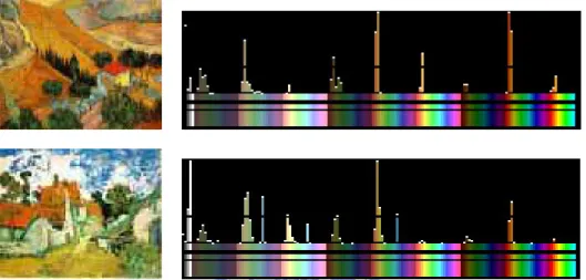
(20) given as follows [16] Y = 0.299* R + 0.587 * G + 0.114* B I = 0.596* R − 0.275* G − 0.321* B Q = 0.212* R − 0.523* G + 0.311* B. (2.3). Because YIQ color space is derived from YUV color space, it is frequently used for image compression and video compression applications.. 2.1.1.4 Luv color space. The CIE Luv color space [17] which component are L*, u* and v*. L* component defines the luminance, and u*, v* define chrominance. The CIE Luv color space represented in terms of XYZ space (another color space defined by CIE). A primary benefit of using Luv color space is that the perceived difference between any two colors is proportional to the geometric distance in the color space between their color values. Thus, Luv color space is very used in calculation of small colors or color differences, especially with additive colors.. 2.1.2 The Feature of Color Image. Human visual system can recognize object by the color information. Therefore, we can describe an color image using the color features such as color histogram, color moment, and texture, etc. Visual Description Tools [18] included in the standard MPEG-7 consist of structures and descriptors that cover the following basic visual features：Color, Texture, Shape, Motion, and Localization, etc. In this section, we will introduce these features. They are widely used in image retrieval.. 2.1.2.1 Color Histogram. Color histogram is the most frequently used color feature. The advantage of color histogram is that it operation is simple. Moreover, color histogram is invariant to translation, rotation, and scaling of an image. A histogram counts the number of pixels of each color bin. 10.

(21) A simple and coarse method of creating a histogram to represent a color image is to quantize the RGB color space so that the number of color bins will be more proper for computing. Because color histogram is a global color feature without spatial information, a drawback of color histogram representation is that information about object location, shape, and texture is discarded. There have two different images with the similar color histograms as Fig. 2-3 shows.. Fig. 2-3. Two different images with similar color histograms. The histogram intersection was proposed for measure the similarity of color histograms in image retrieval [19]. For example, measured the similarity of image I and model image M , the normalized intersection of image histogram h( I ) and model histogram h( M ) is defined as the sum of the minimum over all K corresponding bins and divide the size of model image M as follows. ∑ intersection(h( I ), h( M )) =. K j =1. min {h( I )[ j ], h( M )[ j ]}. ∑ j =1 h(M )[ j ] K. (2.4). Where h( I )[ j ] is the number of pixels in the image I with the intensity j.. 2.1.2.2 Color Moments. The color distribution of an image can be characterized by color moments. If the value 11.

(22) of the i-th color channel at the j-th image pixel is pij then the first three moments are： Ei =. 1 N. N. ∑p j =1. (2.5). ij 1. ⎛1 σi = ⎜ ⎝N. ∑( p. − Ei ). ⎛1 si = ⎜ ⎝N. ∑( p. − Ei ). N. ij. j =1. 2. ⎞2 ⎟ ⎠. (2.6). 1. N. j =1. ij. 3. ⎞3 ⎟ ⎠. (2.7). The first moment, Ei , defines the average intensity of each color component. The second and third moment, σ i and si , define the variance and skewness of each color component. Let H and I be the color distributions of two images with r color components. The first three moments of H and I are Ei , σ i , si and Fi , ς i , t i , respectively. Then, the similarity measure is the weighted Euclidean distance [20] defined as： r. d mom ( H , I ) = ∑ ( wi1 Ei − Fi + wi 2 σ i − ς i + wi 3 si − ti ), i =1. wkl ≥ 0 (1 ≤ k , l ≤ 3). (2.8). The advantage of using color moments is it can overcome the quantization effects. However, color moments also are global features of an image. So only using color moments as the color features of image is not enough for image retrieval.. 2.1.2.3 Texture. Texture refers to the visual patterns that have some properties of homogeneity. In 1973, Haralick proposed two-dimensional co-occurrence matrices for texture analysis because they are able to capture the spatial dependence of gray-level values within an image [21]. A 2D co-occurrence matrix, P, is an n x n matrix, where n is the number of gray-levels within an image. The matrix acts as an accumulator so that P[i , j] counts the number of pixel pairs having the intensities i and j. Pixel pairs are defined by a distance and direction which can be represented by a displacement vector d =(dx,dy), where dx represents the number of pixels moved along the x-axis, and dy represents the number of pixels moved along the y-axis of an 12.

(23) image. A co-occurrence matrix P of image I is defined as. P[i, j ] = {[ x, y ] I [ x, y ] = i and I [ x + dx, y + dy ] = j}. (2.9). Normalizing the co-occurrence values to lie between zero and one allows them to be thought of as probabilities in a large matrix [22]. The normalized co-occurrence matrix N is defined by N [i, j ] =. P[i, j ] ∑∑ P[i, j ] i. (2.10). j. In order to quantify this spatial dependence of gray-level values, we calculate various textural features from the normalized co-occurrence matrix, including Entropy, Energy (Angular Second Moment), Contrast, Homogeneity, SumMean (Mean), Variance, and Correlation as follows： Entropy = −∑∑ N [i, j ]log N [i, j ]. (2.11). Energy = ∑∑ N 2 [i, j ]. (2.12). contrast = ∑∑ (i − j ) 2 N [i, j ]. (2.13). N [i, j ] 1+ i − j. (2.14). i. i. j. j. i. j. Homogeneity = ∑∑ j. i. ∑∑ (i − µ )( j − µ ) N [i, j ] i. correlation =. i. j. j. (2.15). σ iσ j. where µi , µ j are the means and σ i , σ j are the standard deviations of the row and column sums N [i ], N [ j ] define by N [i] = ∑ N [i, j ] j. N [ j ] = ∑ N [i, j ]. (2.16). i. To choose the displacement vector d, we can use χ 2 statistical test [22] to select the value of d that have the most structure. In other words, the displacement vector d that maximizes the. following value should be selected. 13.

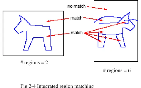
(24) χ 2 (d ) = ∑∑ i. j. N 2 [i, j ] −1 N [i ]N [ j ]. (2.17). 2.1.3 Region-Based Image Retrieval. In this section, we will examine some proposed region-based image retrieval systems. It is beneficial to consider some issues on these topics. We will discuss them in details.. 2.1.3.1 IRM：Integrated Region Matching for Image Retrieval. Li and Wang proposed IRM [1], a novel similarity measure for region-based image similarity comparison. The IRM has been implemented as a part of SIMPLIcity image retrieval system [13]. IRM first segments the image into blocks of 4x4 pixels and extracts a feature vector for each block. The k-means algorithm is used to cluster the feature vectors into one region in the segmented image. Six features are used for segmentation. Three of them are the average color components (LUV color space) in a 4x4 block. To obtain the other three features, a Daubechies-4 wavelet transform is applied to the L component of the image. After a one-level wavelet transform , the image is decomposed into four frequency bands： LL, LH, HL, and HH bands. The other three features are the energy in high frequency bands of the wavelet transform. The distance between a region pair is determined by color, texture, and shape of the regions. The mean values of cluster feature vectors are used to represent color and texture in one corresponding region. To describe shape, normalized inertia of order 1 to 3 are used. They are invariant with scaling and rotation. When measuring the similarity between two images, we should be aware that segmentation cannot be perfectly, the matching is “softened” by allowing one region of an image to be matched to several regions of another image. That is, the region mapping between any two images is a many-to-many relationship, as illustrated in Fig 2-4 [13]. As a result, the. 14.

(25) similarity between two images is defined as the weighted sum of distances in the feature space, between all regions from different images.. # regions = 2 # regions = 6 Fig 2-4 Integrated region matching. The advantage of IRM is that, in order to increase the robustness against inaccurate segmentation, IRM allows a region to be matched to several regions in another image. Each of the matching is assigned with a significance credit which corresponds to the importance of the matching. There are several ways to assign the importance of a region. One can assume that every region is equally important. IRM views that important objects in an image tend to occupy larger areas, called an area percentage scheme. This scheme is less sensitive to inaccurate segmentation than the uniform scheme. If one object is partitioned into several regions, the uniform scheme raises its significance improperly, whereas the area percentage scheme retains its significance to the region. The authors compared IRM with the WBIIS (Wavelet-Based Image Indexing and Searching) system [7] using the same image database. WBIIS forms image signatures using wavelet coefficients in the lower frequency bands and performs well with relatively smooth images. For images containing detail semantics, such as pictures containing people, the performance of WBIIS degrades. In general, the IRM system performed well both in smooth 15.

(26) images and images composed of fine details.. 2.1.3.2 Research Issue. There are some aspects that affect the effect of a region-based image retrieval system, we list them as follows and discuss them in details. Color model：. When we choose a color model to represent color information, we should consider what kind of color model can make retrieval operations more perfectly. A good color model should separate different color information from each other effectively, because it will beneficial to consequent operations. For example, when segmenting an image into regions, if color information can be separated clearly then the clustering algorithm can, according to different color information, achieve semantic segmentation. The usually used color models are YIQ, HSI, and L*a*b* [23]. Image segmentation：. Semantic segmentation of the image content and concise representation of the essence of the data are crucial steps for image retrieval. Inaccurate segmentation will conduce non-exactly features to describe regions, even though optimal semantic segmentation is difficult to achieve. The usually used clustering algorithm in region-based image retrieval are k-means, KMCC [24], watershed [25], and JSEG [26]. Feature extraction：. Most image retrieval systems often use features of color, shape, and texture, etc. For instance, MPEG-7 Visual Description [18] uses Color, Texture, Shape, Motion, and Localization to describe regions. We should pick the proper features and tune the weights of features semantically. According to different image database, we should set different feature weights. For example, shape feature is not perceptually important when retrieval textured images, and the weights corresponding to color features should be set higher values when 16.

(27) retrieval colorful images. Note that the dimension of feature vectors will affect the time of extracting features from regions. Thus there is an issue need to consider is the time of image segmentation. In recent years, the size of digital image collections is increased rapidly. This size is proportional to the time of image segmentation and feature extraction, thus it should be considered if we want a real-time retrieval system. Similarity measure：. The way of query mode can be classified into“Query by single region＂and“Query by all regions＂in region-based image retrieval system. Many researches indicate that systems using “Query by all regions” mode has been proven more effective than those using “Query by single region” mode during the retrieval process. Because “Query by all regions” mode can reduce the influence of inaccurate segmentation when measuring similarity values. Besides, when system using “ Query by single region＂mode, if there are some images without distinctive objects or scenes, it is difficult for users to determine which regions and features should be used for retrieval. Next, we need to consider how to compute the similarity distance between images. The IRM [1] uses significance matrices in the similarity distance algorithm. The significance matrix is determined by the importance of the object which means the area percentage of an object to the entire image. In another region-based image retrieval system proposed by Zhang [27], suggested only matching regions that have the smallest distance to other regions in another image during similarity distance computation. Additionally, Zhang also added the weight during the matching process to determine the importance of the object compared to the entire image.. 2.2 Wavelet Transform and Multiresolution Processing. In recent years, many studies indicated that wavelet transform is easier to compress, 17.

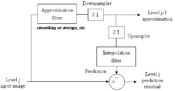
(28) transform, and analyze images than the Fourier transform。In this section, we will introduce wavelet transform from its foundation – multiresolution theory to discrete wavelet transform. The main purpose of multiresolution is to represent and analyze an image in various resolutions by reason of that some information or feature reveals only in particular resolution.. 2.2.1 Image Pyramid. Multiresolution theory is concerned with the presentation and analysis of signals (or images) at more than one resolution [15]. Image pyramid is a conceptually simple structure to represent an image in different resolutions. An image pyramid is a collection of decreasing resolution image arranged in the shape of a pyramid [28], as illustrated in Fig 2-5.. Fig.2-5. A pyramidal image structure The system block diagram of image pyramid decomposition and synthesis is illustrated in Fig 2-6 [15]. When decomposing an image f n with size 2 N × 2 N , we first calculate the approximation image fˆn and downsample it to size 2 N −1 × 2 N −1 , which is then used as the input image f n −1 of the next level decomposition process. We upsample f n −1 back to size ~ ~ 2 N × 2 N , denoted by f n , then calculate the difference en = f n − f n . By iteratively applying 18.

(29) this process, we will get a series of differences en , en −1 , …, e2 , e1 and a level 0 image f 0 . When transferring the source image via the network, we first send f 0 and then consequently send e1 , e2 , …, en −1 , en in turn. When combining the subimages in the receiver, we first upsample the subimage f 0 to ~ ~ f1 ’s approximation, f1 of size 2x2, then calculate f1 = f 1 + e1 for reconstructing the image of the previous level. After iteratively applying this process in each level, the original image will finally be obtained.. Fig. 2-6 System block diagram for creating an image pyramid.. The efficiency of storage and concurrency of the reconstructed image depend on the approximation filter in the multiresolution decomposition system. There are various approximation filters to be utilized in the system, including neighborhood averaging for producing a mean pyramid, lowpass Gaussian filtering for producing a Gaussian pyramid, or no filtering for producing a subsampling pyramid.. 2.2.2 Discrete Wavelet Transform. Wavelet transform represents an image as a sum of wavelet functions with different 19.

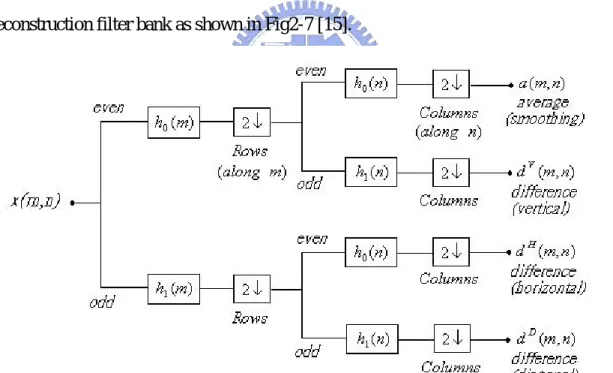
(30) locations and scales [29]. Any decomposition of an image into wavelets involves a pair of waveforms: one to represent the high frequencies corresponding to the detailed parts of an image (wavelet function Ψ ) and one for the low frequencies or smooth parts of an image (scaling function Φ ). Discrete wavelet transform (DWT) for an image as a 2-D signal can be derived from 1-D DWT. The easiest way for obtaining scaling and wavelet function for two dimensions is by multiplying two 1-D functions. The scaling function for 2-D DWT can be obtained by multiplying two 1-D scaling functions： Φ ( x, y ) = Φ( x)Φ( y ) .Wavelet functions for 2-D DWT can be obtained by multiplying two wavelet functions or wavelet and scaling function for 1-D analysis. For the 2-D case, there exist three wavelet functions that scan details in horizontal： Ψ ( I ) ( x, y ) = Φ ( x)Ψ ( y ) , vertical： Ψ ( II ) ( x, y ) = Ψ ( x)Φ ( y ) , and diagonal directions ： Ψ ( III ) ( x, y ) = Ψ ( x)Ψ ( y ) . This may be represented as a four-channel perfect reconstruction filter bank as shown in Fig2-7 [15].. Fig. 2-7 Two-dimensional four-band filter band.. By using these filters in one stage, an image can be decomposed into four bands. There are three types of detail images for each resolution: horizontal (HL), vertical (LH), and diagonal (HH). The operations can be repeated on the low–low band using the second stage of. 20.

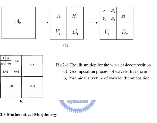
(31) identical filter bank. The decomposition process is illustrated as Fig2-8 (a). Thus, a typical 2-D DWT, used in image compression, will generate the hierarchical pyramidal structure shown in Fig2-8 (b).. (a). Fig 2-8 The illustration for the wavelet decomposition (a) Decomposition process of wavelet transform (b) Pyramidal structure of wavelet decomposition. (b) 2.3 Mathematical Morphology. Mathematical morphology is a tool for extracting image components that are useful in the representation and description of region shape, such as boundaries, skeletons, and the convex hull. Mathematical morphology is a set-theoretic method. Sets in mathematical morphology represent the shapes of objects in an image. The operations of mathematical morphology were originally defined as set operations and shown to be useful for image processing. In general, morphological approach is based upon binary images. In binary images, each pixel can be viewed as an element in Z 2 . Gray-scale digital images can be represented as sets whose components are in Z 3 , two components are the coordinates of a pixel, and the third corresponds to its discrete intensity value. The morphological operations input a source 21.

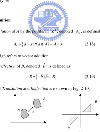
(32) image and a structuring element which is another image usually smaller than source image. The structuring element is a predetermined geometric shape, and there are some common structuring elements as shown in Fig. 2-9. 1. 1. 1. 1. 1. 1. 1. 1. 1. 1 1. 1. 1. 1. 1. 1. 1. 1. 1. 1. 1. 1. 1. 1. 1. 1. 1. 1. 1. 1. 1. 1. 1. 1. 1. 1. 1. 1. 1. 1. 1. 1. 1. 1. 1. 1. 1. 1. 1. 1. 1. 1. Fig. 2-9 Examples of structuring elements Here, we will discuss morphological operators in binary images [30, 31]. Given a source image A and a structuring element B in Z 2 , with components a and b respectively. And φ denotes the empty set.. 2.3.1 Basic definition. The Translation of A by the point x in Z 2 , denoted AxK , is defined by K K K K AxK = {a + x | ∀a ∈ A} = A + x. (2.18). where the plus sign refers to vector addition. And the Reflection of B, denoted Bˆ , is defined as K K B = −b | b ∈ B. {. }. (2.19). The examples of Translation and Reflection are shown in Fig. 2-10. AxK. B. K x. A. Bˆ. (a). (b). Fig. 2-10 Examples of (a) Translation and (b) Reflection 22.

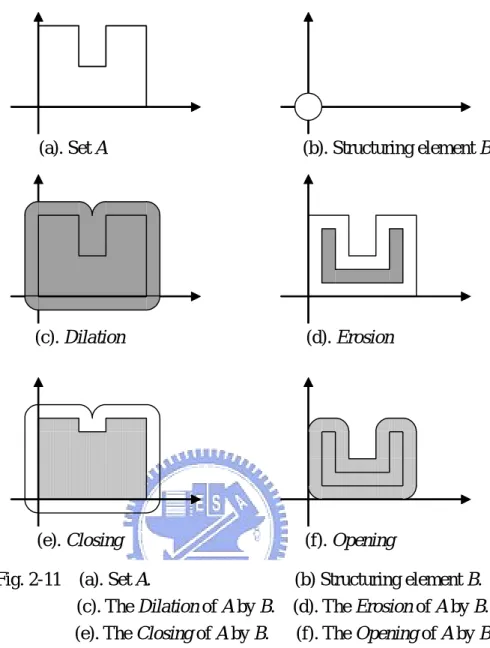
(33) 2.3.2 Morphological operations. Here, we introduced two of the fundamental morphology operations：Dilation and Erosion used in binary images, and introduced two operators：Closing and opening that extended from Dilation and Erosion. The Dilation of A by B, denoted D B ( A) , is defined as. {. K K DB ( A ) = A ⊕ Bˆ = x | Bˆ + x ∩ A ≠ φ. }. (2.20) .. Where B is the structuring element. And the Erosion of A by B, denoted E B ( A) , is defined as K K EB ( A ) = A0 B = { x | B + x ⊂ A}. (2.21) .. The examples of Dilation and Erosion are shown in Fig. 2-11(c) and (d). The dilation of A by. K B is the set of all x displacements such that Bˆ and A overlap by at least one nonzero K K element. The erosion of A by B is the set of all points x such that B translated by x is contained in A. The Closing of set A by structuring element B, denoted C B ( A) , is defined as. (. ). CB ( A ) = A • B = EBˆ ( DB ( A ) ) = A ⊕ Bˆ 0 Bˆ. (2.22) .. And the Opening of set A by structuring element B, denoted O B ( A) , is defined as OB ( A ) = A D B = DBˆ ( EB ( A ) ) = ( A0 B ) ⊕ B. (2.23) .. The examples of Closing and Opening are shown in Fig. 2-11(e) and (f). The closing of A by. B is simply the dilation of A by B, followed by the erosion of the result by Bˆ . The opening of A by B is simply the erosion of A by B, followed by the dilation of the result by Bˆ .. 23.

(34) (a). Set A. (b). Structuring element B. (c). Dilation. (d). Erosion. (e). Closing. (f). Opening. Fig. 2-11 (a). Set A. (b) Structuring element B. (c). The Dilation of A by B. (d). The Erosion of A by B. (e). The Closing of A by B. (f). The Opening of A by B.. 2.3.3 Extension to Gray-Scale Images. In this section we extend to gray-level images the basic operations of dilation, and erosion. Throughout the discussions that follow, we deal with digital image functions of the forms f ( x, y ) and b( x, y ) , where f ( x, y ) is the gray-scale image and b( x, y ) is a structuring element. Gray-Scale dilation of f by b , denoted by f ⊕ b , is define as： ( f ⊕ b)( s, t ) = max{ f ( s − x, t − y ) + b( x, y ) ( s − x), (t − y ) ∈ D f ;( x, y ) ∈ Db }. (2.24). Where D f and Db are the domain of f and b , respectively. As before, b is the structuring. 24.

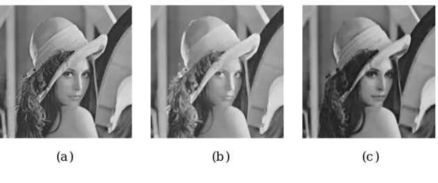
(35) element of the morphological process but note that b is now a function rather than a set. Because dilation is based on choosing the maximum value of f + b in a neighborhood defined by the shape of the structuring element, the general effect of performing dilation on a gray-scale image is two-fold: (1) if all the values of the structuring element are positive, the output image tends to be brighter than the input; and (2) dark details either are reduced or eliminated, depending on how their values and shapes relate to the structuring element used for dilation. As illustrated in Fig 2-12 (b). Gray-scale erosion of f by b , denoted by f 0b , is define as： ( f 0b)( s, t ) = min{ f ( s + x, t + y ) − b( x, y ) ( s + x), (t + y ) ∈ D f ;( x, y ) ∈ Db } (2.25) Where D f and Db are the domain of f and b . Because erosion is based on choosing the minimum values of f − b in a neighborhood defined by the shape of the structuring element, the general effect of performing erosion on a gray-scale image is two-fold: (1) if all the values of the structuring element are positive, the output image tends to be darker than the input; and (2) bright details are reduced or eliminated, depending on the used structuring element. As illustrated in Fig 2-12 (c).. (a ). (b ). (c ). Fig. 2-12. (a) The original of Lena image (b) Dilation of Lena image (c) Erosion of Lena image. 25.

(36) The usage of closing and closing is to smooth contours of objects. In gray-level images, closing is used for brighter objects with darker background, and opening is used for darker object objects with brighter background. As illustrated in Fig 2-13 (b) and (c).. (a ). (b ). (c ). Fig. 2-13. (a) The original of Lena image (b) Closing of Lena image (c) Opening of Lena image 2.3.4 Morphological Gradient. The Morphological Gradient of an image, denoted G: G = DB ( A ) − EB ( A ) = ( A ⊕ B ) − ( A0 B ). (2.26). or G = DB ( A ) − A = ( A ⊕ B ) − A. (2.27). G = A − EB ( A ) = A − ( A0 B ). (2.28) .. or. The morphological gradient highlights sharp gray-scale transitions in the source image. In other words, morphological can extract the boundary of an object. However, the morphological gradient is sensitive to the shape of the chosen structuring element. Here are examples of dilation, erosion, closing, opening, and morphological gradient of the gray-scale. 26.

(37) image, Lena, with the 3×3 structuring element as shown in Fig 2-14.. (a ) (b ) Fig. 2-14. (a) The original of Lena image (b) Morphological gradient of Lena image. 27.

(38) CHAPTER. 3. The Proposed Method. In this chapter, we will introduce the architecture of the retrieval system based on our proposed method. In section 3.1, we will discuss the process of our image retrieval. It is know [32] that representing an image as a combination of multiple regions is advantageous than processing an image as a single entity. Moreover, the local features can be easily measured and more semantically described by regions. Thus, in section 3.2, we will utilize K-means clustering algorithm to automatically segment an image into regions. In section 3.3, we will introduce methods for extracting texture, color and shape features from regions. In section 3.4, our overall image similarity measure will be defined.. 3.1 Overview of Our Image Retrieval System. Our image retrieval system is a class of “Query by Example” system, so each user needs to input a query image at the start of the retrieval process. As illustrated in Fig 3-1, when an user choose a query image from the image database, the system will segment the query image into several regions and extract texture, color and shape features from these regions. Similarity, the system will do the same operations on each image in the image database, then store the extracted features to form the feature database for retrieval usage. When an user wants to do retrieval, the system will compare the features of the query image with all features in the feature database to compute each of similarity values. At last, the system will sort the images in descending order by the similarity values and present retrieval results on the interface. When an user considers a retrieved image as an irrelevant one, he can mark it as an irrelevant image, and the system will utilize relevance feedback technique to recomputed the weights of regions, then the retrieval process starts again. 28.

(39) Query image. Image segmentation. Feature extraction. Similarity measure. Irrelevant image No Distance ≤ Threshold Yes. Images in the database. Image segmentation. Feature extraction. Relevance feedback. Rank Generator. Result output. Fig3-1. Overview of Our Image Retrieval System. 3.2 Image Segmentation. The most important part in region-based image retrieval is image segmentation, because semantic segmentation of the image content and concise representation of the essence of the data are crucial steps for image retrieval. So in this section, we will discuss image segmentation in details.. 3.2.1 K-means Clustering Algorithm and Cluster Number. Before doing image segmentation, we need to transform RGB color model into other color model in order to make segment more semantically. We take the YIQ color space as the color model due to the fact that the YIQ color space is more related to the human perception. After splitting the input image into three color components, the wavelet transform is applied to each component. Then we will utilize clustering algorithm in LL subband for image segmentation. The image segmentation process is illustrated using Fig3-2.. 29.

(40) (a). (b). (c). Fig3-2.The process of image segmentation (a) Original image (b) Clustering algorithm applied in the LL subband (c) Final segmentation result In our method, we applied the K-means clustering algorithm [33] in the LL subband. In order to achieve semantic segmentation, the distance function in the K-means clustering algorithm will include color and texture information. So the cluster feature vector is composed of the YIQ color components of LL subband, and the IQ components of HL3 、 LH 3 、 HH 3 subbands. The cluster feature vector of a pixel at (x , y) is defined as a 9-tuple vector： S x , y = ⎡⎣ s1x , y , sx2, y ..., sx9, y ⎤⎦ I 3 I 3 I 3 Q Q Q = ⎡ sYx ,LLy , sxI LL, y , sxQ,LLy , sxHL , sxLH , sxHH , sx ,HLy 3 , sx ,LHy 3 , sx ,HHy 3 ⎤ y y y , , , ⎣ ⎦. (3.1). The motivation for using the last six features is their reflection of texture information in high frequency subbands. If we segment image into K clusters, we will have K cluster centers ci , i = 1,..., K , the K-means clustering algorithm is describe as below： Step 1. Initialize the cluster centers： Randomly choose K points (x , y) as the cluster centers. ci = ( x, y ), i = 1,..., K ;0 ≤ x ≤ the height of image , 0 ≤ y ≤ the width of image Step 2.Compute the distance function： ( x, y ) ∈ R j , if S x , y − Sc j ≤ S x , y − Sci , for all i = 1,..., K ; i ≠ j Where R j denotes the set of pixels whose cluster center is c j , j = 1, 2,..., K Step 3. Compute the new cluster centers：. 30. (3.2).

(41) The new cluster center for class j is give by c 'j =. 1 Nj. ∑ ( x, y ) , j = 1,..., K. (3.3). ( x , y )∈R j. Where N j is the number of pixels in R j . Recompute the new cluster center make the sum of the squared distances from all points in R j to the new cluster center be minimized. Step 4. If c 'j = c j , j = 1,..., K then the algorithm is terminated, otherwise go to Step 2. We iterate the above algorithm between minimum cluster number K=3 to maximum cluster number K=8. We do not apply the K-means algorithm when K is less than 3, because natural images usually are composed of many different color objects. The ”optimal” cluster number K is determined by the method proposed by [34] . The kernel of this method is to make the clusters as compact as possible. First, we define the intra-cluster distance measure to be the distances between points to its cluster center divided by the total number of pixels. That is, Intra =. 1 N. K. ∑ ∑ ( x, y ) − c. (3.4). i. i =1 ( x , y )∈Ri. Where N is the number of pixels in the image, ci is the cluster center of cluster Ri . Then we define the inter-cluster distance measure to be the minimum distance between cluster centers. That is, Inter = min( ci − c j ), i = 1, 2,....., K − 1, j = i + 1,...., K. (3.5). Our aim is to minimize the intra-cluster distance and maximize the inter-cluster distance such that the clusters can be more compact. If we take the ratio, called the validity, validity =. Intra Inter. (3.6) ,. then the clustering which gives a minimum value for the validity will be the optimal value of K in the K-means clustering algorithm.. 31.

(42) 3.2.2 Color Image Segmentation by K-means Algorithm. In this section, we will show some segmentation result and discuss some related details. When computing distance function in K-means algorithm, we have to decide the weight w j to every sub-cluster feature vector in the following formula： S x , y − Sci =. ∑ w *(s 9. j =1. j. j x, y. ). − scji , ci is the cluster center. (3.7). Because I and Q components are the chromaticity values, if we set higher values to weights which map to the I and Q components of cluster feature vectors we can get more precise segmentation results, so we will discuss the weight map to Y component ( w1 ) and I、Q component ( wi , i = 2,...,9 ) separately. Fig 3-3 and Fig 3-4 show the results of segmentation with different values of wi .. (a). (b) Fig3-3.Example of segmentation results (a) Original image (b) Segment with wi = 1, i = 1,...,9 (enlarge to 16 times) (c) Segment with w1 = 1; wi = 4, i = 2,...,9. (c). (enlarge to 16 times). 32.

(43) (a). (b) Fig3-4.Another example of segmentation results (a) Original image (b) Segment with wi = 1, i = 1,...,9 (enlarge to 16 times) (c) Segment with w1 = 1; wi = 4, i = 2,...,9. (c). (enlarge to 16 times). In the segmentation process, we set one gray-value to one region in order to distinguish regions from each other. From experiment results, we can clearly see that by setting higher values to weights corresponding to the I and Q components of cluster feature vectors, we can have more precise segmentation results.. 3.3 Feature Extraction of Region. After segmenting the objects and labeling by region, we extract features from wavelet coefficients to describe region content. In order to describe region content more exactly, it is necessary to combine the information in all the different frequency subbands. High frequency subbands are desired because they include finer visual features. Referring to Fig3-5 [32], for one segmented region Ri in the LL subband, we find its corresponding region in the same spatial location at the HL3 、 LH 3 、 HH 3 subbands. Then utilizing spatial orientation tree structure described in Fig3-5 (b), we localize their corresponding regions at the other high frequency subbands described in Fig3-5 (c). We will combine texture, color and shape features of these sub-regions in wavelet domain to describe Ri content more semantically.. 33.

(44) (a). (b). (c). Fig3-5 The illustration for the generation of hierarchical region feature vector. (a) One region in an image (b) Spatial orientation tree: The arrow points from the subband of the parents to the subband of the children (c)Corresponding regions in wavelet domain. In our method, we utilize the energy of wavelet coefficients and morphological operation on wavelet coefficients to define region feature vectors. Our region feature vectors include texture, color and shape features. Texture features attribute to the energy of wavelet coefficients, while color and shape features attribute to morphological operation on wavelet coefficients.. 3.3.1 Texture Feature. Many researches indicate that the energy of wavelet coefficients in the high frequency subbands is effective for discerning texture, and wavelet coefficients are not invariant with respect to translation, rotation and scaling of the image. Thus, we adopted the energy of wavelet coefficients to describe texture features of regions. The local energy E p of one sub-region in the pth subbands, calculated from its three color local energy components, E pY , E pI , E pQ , is defined as E p = wY *log( E pY ) + wI *log( E pI ) + wQ *log( E pQ ), p = 1, 2,...P. (3.8). where P is the total number of subbands with the wavelet decomposition level L, 34.

(45) P = 3* L + 1 . In order to emphasize the color properties, we will set higher values to. wI and wQ . Experiment results (see chapter 4) will demonstrate that emphasizing wI and wQ can conduce better retrieval results. We will discuss this in chapter 4. The E pY is defined as follows：. E pY =. ∑ (C ). m , n∈S. 2 Y m,n. (3.9). Here CmY ,n is the Y color component of wavelet coefficient Cm,n in the wavelet domain, S indicates the sub-region in the pth subbands. The E pI and the E pQ are also defined as the similar ways. At last we obtain the representative texture feature vector [ E1 , E2 ,....., EP ] for region Ri from above equation.. 3.3.2 Color and Shape Feature. After obtaining texture features, we will use morphological operations on wavelet coefficients to get color and shape features. We adopted morphological operations because they only involve simple logical operations and can reduce the computing time of feature extraction. In our method, we use dilation, erosion, and gradient operators to get color features. In gray-level images, dilation can be seen as a “max” operation on pixels. Similarly, erosion can be seen as a “min” operation. These two operators can get the color information, while the gradient operator can get shape information of regions. Note that an edge pixel will have a high morphological gradient value, and a pixel on a flat region will have a low value. Thus, we can use these three operators to define color feature vectors that describe color and shape information of regions. These color feature vectors are defined as： ⎧1 FD = ⎨ ⎩N. ∑. m , n∈S. DB ( CmY ,n ),. 1 N. ∑. m , n∈S. DB ( CmI ,n ),. 35. 1 N. ⎫ DB ( CmQ, n ) ⎬ m , n∈S ⎭. ∑. (3.10).

(46) ⎧1 FE = ⎨ ⎩N ⎧1 FG = ⎨ ⎩N. ∑. m , n∈S. EB ( CmY ,n ),. 1 N. ∑. m , n∈S. EB ( CmI ,n ),. 1 N. ⎫ EB ( CmQ,n ) ⎬ m , n∈S ⎭. ∑. ⎫. ∑ G ( C ), N ∑ G ( C ), N ∑ G ( C )⎬. m , n∈S. B. Y m,n. 1. m , n∈S. B. I m,n. 1. m , n∈S. B. Q m,n. ⎭. (3.11). (3.12). Where B is a structuring element, DB , EB , and GB are Dilation, Erosion, and Gradient operator, respectively. CmY ,n is the Y color component of wavelet coefficient Cm ,n in the wavelet domain, S indicates the sub-region in the LL subband, N is the number of pixel in sub-region in the LL subband. At last we obtain the representative color feature vector. [ FD , FE , FG ]. for region Ri from above equation.. 3.3.3 Region Feature Vector. Finally, we combine texture feature and color and shape feature to compose of region feature vector. FV Ri that describe region Ri as JJK JJK JJK FV Ri = ⎡⎣ FD , FE , FG , E1, E2 ,...., EP ⎤⎦. (3.13). Our region feature vectors have two advantages： 1. Region feature vector can characterize the region content more exactly because it combines texture, color and shape information of the region. 2. The feature components in the region feature vector can be tuned semantically and effectively.. 3.4 Similarity Measure. In this section, we first define the similarity measure between two regions, then extend to define the overall similarity measure between two images. When computing the distance between two region feature vectors, the proper weight adjustment for feature components in. 36.

(47) the feature vectors is important for region similarity measurement. We use distance function to measure the similarity between two regions ( Ri and R j ), which is defined as Dis ( Ri , R j ) = wc * sc + wt * st ⎛ R = wc * ⎜ wD * FDRi − FD j ⎝. (. ⎛ + wt * ⎜ ⎜ ⎝. ∑ w *( E P. k =1. Ri k. k. ). 2. − Ek j R. (. + wE * FERi − FE j. ). 2. R. ). 2. (. + wG * FGRi − FG j R. ). 2. ⎞ ⎟ ⎠. (3.14). ⎞ ⎟⎟ ⎠. Where wc is the weight of color feature, wt is the weight of texture feature; wD , wE , and wG are the weight of dilation, erosion, and gradient operator, respectively; wk is the weight of sub-texture feature vector, P is the total number of subbands. Experiment result demonstrates that when we set larger value to wt than wc , we will get better precision in the retrieval process. Besides, because LL subband is the main color and texture information of visual significant objects in image, we will set weight w1 larger. Then we start to define the overall similarity measure between two images. For example, suppose we have the query image Q and one image D in the database. First, for each region Ri in image Q, we calculate the minimum distance between it and all the regions in image D, by Distance ( Ri , R j ) = min ( Dis( Ri , R j ) ) , Ri ∈ Q , R j ∈ D j. (3.15). Next, the overall image similarity is measured as the sum of the similarity between similarly region pairs, by Sim(Q, D) =. ∑. i∈Q , j∈D. λi , j * e. − Distance ( Ri , R j ). (3.16). Where λi , j is a significance value considered as the effect of region sizes for the image similarity measure. The λi , j for one region pair Ri in query image Q and R j in image D in the database, is defined as. 37.

(48) λi , j =. size( Ri ) + size( R j ) size( Ri ) / size(Q) * size(Q) + size( D) size( R j ) / size( D). (3.17). Where size( R) is the number of pixels inside the region R . The first item takes into account the relative sizes of the regions with respect to the images they belong to, and the second item takes into account the similarity of sizes between two regions. In this way, this definition can make overall image similarity measure more effectively. In order to avoid the outlier appearance, we only take into account the regions which sizes are not too small and the morphological operator values of the regions cannot be zero. A graphical explanation of overall image similarity measure is illustrated in Fig 3-6.. R1. R2. R3. R4 Image 1. λ 2,4. λ 1,1. Image 2. R1. R2. R3. R4. Fig 3-6 .The illustration of overall image similarity measure The line connecting Ri and R j denotes Distance( Ri , R j ) Then for the query image, the image indexing system measures the image similarity between it and each image in the database. Then the system sorts the images in descending order by the similarity values and present retrieval result on the interface.. 38.

(49) CHAPTER 4 Experimental Results 4.1 Experiment Environment. In this chapter, we will present some experimental results obtained by applying the proposed method described in chapter 3. The experimental database includes 1000 general-purpose photography color images come from 10 categories with sizes 384x256 or 256x384, which are gathered from the COREL photo library. Each category contains 100 images. These 10 categories consist of the model, beach, buildings, buses, dinosaurs, elephants, flowers, horses, under water, and food. Fig. 4-1 shows several example images of each class from the database.. Class 1. Class 2. Class 3. Class 4. Class 5. Class 6. Class 7. Class 8. Class 9. Class 10. Fig 4-1 The examples of the image database 39.

(50) In our method, we use Daubechies 9-7 filter in wavelet transform, and wavelet decomposition level is set to 3. When we extract color and shape features, the structuring element of morphological operators is a 3x3 filter. The proposed method is implemented on PC with Pentium4 1.8G, RAM 512 Megabytes. The first experiment verifies the effectiveness of emphasizing I and Q components when extract texture features. The second experiment demonstrates that after combining texture feature with color and shape feature, our image retrieval system will get higher precision. The third experiment verifies the robustness of our image retrieval system. Finally, we implement the relevance feedback technique proposed by Shin [35] in our image retrieval system.. 4.2 The First Experiment. In the first experiment, we will verify the effectiveness of emphasizing I and Q components in our image retrieval system. We use equation 3-8 to extract texture features and to describe regions, because I and Q components are the chromaticity values and the image database consist of natural images that are colorful, if we set higher values to weights which map to the I and Q components of texture feature in equation 3-8, we can get higher precision. Here we only use texture feature being our feature vector. In Fig 4-2(a), we set wY , wI , and wQ the same weight value in equation 3-8. On the other hand, in Fig 4-2(b), we emphasize the wI and wQ more than wY in equation 3-8. Fig 4-3 is another example to verify the effectiveness of emphasizing I and Q components. From experiment results, we can see that by setting higher values to weights corresponding to the I and Q components of texture features, we can get more relevant images and color properties of retrieved images are more similar with query image.. 40.

(51) (a). (b) Fig 4-2 The example of emphasize I and Q component in texture feature (a)The retrieval result of wY , wI , and wQ are the same weight value (b)The retrieval result of set higher weight value to wI and wQ more than wY. 41.

(52) (a). (b) Fig 4-3 Another example of emphasize I and Q component in texture feature (a) The retrieval result of wY , wI , and wQ are the same weight value (b) The retrieval result of set higher weight value to wI and wQ more than wY. 4.3 The Second Experiment 42.

(53) The second experiment verifies that by combining texture feature with color and shape feature, our image retrieval system will get higher precision. Here we use the precision and recall measures to evaluate the effectiveness of the proposed method. Assume that R is the number of retrieved relevant images, T is the total number of relevant images and K is the number of retrieved images, the precision and recall measures are defined as follows: Precision =. R K. (4.1). and Recall =. R T. (4.2). A retrieved image is considered as relevant if and only if it is in the same category as the query image. Here, we evaluated on the COREL database, formed by 10 image categories, each containing 100 pictures. We compare the retrieval that use the feature vector consisted of texture, color and shape feature with the retrieval that only use texture feature being the feature vector. The table 4-1 is the experiment result, when K=20.. Table 4-1 The precision of our image retrieval system using different features. 43.

(54) In our image database, the model, dinosaurs, and under water categories consist of smooth images, on the other hand, the beach, buildings, elephant, and food categories consist of images with fine details. From the second column of table 4-1, the precision of retrieval that only use texture feature being the feature vector, can see the precisions when retrieving images composed of fine details are lower than retrieving smooth images. Because images composed of fine details consist of tiny objects, thus it is difficult to achieve semantically segmentation hence to affect the extracted features. This is why the precision which retrieve the images composed of fine details are lower than retrieve the smooth images. Next, we use the feature vector that consists of texture, color and shape features to retrieve the same image database, the precision is listed in the third column of table 4-1. After comparing two columns from table 4-1, we can clearly see that retrieval using texture, color and shape features will get higher precision than retrieval that only use texture feature, especially when retrieving the smooth images. Because the background of smooth images are colorful, thus we utilize color features to describe them more semantically. It also verifies the effectiveness of morphological operators when extracting color features. Finally, we used precision-recall curves to measure the performance of our image retrieval system, as show in Fig 4-4. In Fig 4-4(a), we use the category 1-model being the test. Because this category consists of smooth images, the precision-recall curves in Fig 4-4(a) will not degrade fast. Next, we use the category 3-buildings being the test. This category belonging to the images composed of fine details, thus the precision-recall curves will degrade fast, as shown in Fig 4-4(b). Because it is difficult to describe tiny objects and decide it’s weights when evaluating similarity measure. Then we compare these two curves in a plot to see more clearly, as shown in Fig 4-4(c).. 44.

(55) (a). precision. category 1:Model 1.2 1 0.8 0.6 0.4 0.2 0 0.01. 0.05. 0.1. 0.15. 0.2. 0.25. 0.3. 0.35. 0.4. recall. category 3:Buildings 1.2. (b). precision. 1 0.8 0.6 0.4 0.2 0 0.01. 0.05. 0.1. 0.15. 0.2. 0.25. 0.3. 0.35. 0.4. recall. category 1. category 3. 1.2. (c). precision. 1 0.8 0.6 0.4 0.2 0 0.01. 0.05. 0.1. 0.15. 0.2. 0.25. recall. Fig 4-4 The precision-recall curves (a) The result of category 1 (b) The result of category 3 (c) Compare category 1 with category 3. 45. 0.3. 0.35. 0.4.

(56) 4.4 The Third Experiment. The third experiment demonstrates the robustness of our image retrieval system. We will do some alternation on query images, such as added noise, shift, mirror, and flip. Fig 4-4 show some query examples, using the 1000-image database. Here added noise is added 10% uniform noise on query image, shift is left shift 20% of original query image, mirror is mirror of the query image, and flip is rotating the query image 180° .. Original image (#401) (a) Add noise. Original image (#809) (b) Shift. Original image (#53) (c) Mirror. 46.