國 立 交 通 大 學
電信工程學系
碩 士 論 文
在高速下行封包擷取系統中
採用乏晰 Q-Learning 技術之混合自動重傳機制
HARQ Process for HSDPA by Fuzzy
Q-learning Technique
研 究 生:黃巧瑩
指導教授:張仲儒 博士
在高速下行封包擷取系統中
採用乏晰 Q-Learning 技術之混合自動重傳機制
HARQ Process for HSDPA by Fuzzy Q-learning Technique
研 究 生:黃巧瑩 Student:Chiao-Yin Huang
指導教授:張仲儒 博士 Advisor:Dr. Chung-Ju Chang
國 立 交 通 大 學
電 信 工 程 學 系
碩 士 論 文
A Thesis
Submitted to Department of Communication Engineering
College of Electrical and Computer Engineering
National Chiao Tung University
in partial Fulfillment of the Requirements
for the Degree of Master of Science
in
Communication Engineering
July 2008
Hsinchu, Taiwan
中華民國九十七年七月
在高速下行封包擷取系統中
採用乏晰 Q-Learning 技術之混合自動重傳機制
研究生:黃巧瑩 指導教授:張仲儒 博士國立交通大學電信工程學系碩士班
摘 要
mimi 1 第三代合作夥伴計畫(3rdgeneration partnership project, 3GPP)在現有的第 三代通訊系統下,提出了一種高速下行封包擷取技術(high speed downlink packet
access, HSDPA)來提供更高速且安全的下鏈路資料封包傳送。HSDPA 採取混合 自動重傳機制(hybrid automatic retransmission request, HARQ)程序,它有一個 重要的服務品質要求:在根據通道狀況決定原始傳送的 MCS 時,必須使其封包 錯誤率小於 0.1。針對這個課題,我們在本篇論文裡利用乏晰 Q 學習演算法來實 現高速下行封包擷取技術之混合自動重傳機制(FQL based HARQ)。在同時考 慮了通道動態調節以及重傳程序的交互影響的情況下,我們將 HARQ 程序模擬 為離散時間馬可夫決策過程(Markov decision process, MDP),經由乏晰系統規 則的設計,來實現 BLER 的服務品質需求,同時利用 Q 學習法,不斷的學習每 一種 MCS 在不同的系統環境下之輸出表現,並修正乏晰系統規則。在學習收斂 後,我們期望可以達到正確的選擇不違反 QoS 需求同時又能達到最高系統輸出 的傳送方式之目的。由模擬結果可以看到,我們所提出的機制可以在有通道訊息 延遲的情況下,對不同的行動用戶通道環境來選擇適當的 MCS,既可滿足 QoS 的需求,又可比傳統只考慮通道動態調節的機制達到更高速的傳輸速率。相較於 其他的比較系統,我們的 FQL-HARQ 可以在滿足 QoS 需求下,獲得最大之系統 輸出。
HARQ Process for HSDPA by Fuzzy Q-learning Technique
Student:Chiao Yin Huang Advisor:Dr. Chung-Ju Chang
Department of Communication Engineering
National Chiao Tung University
ABSTRACT
mimi 2
I
n order to provide higher speed and more effective downlink packet data service in 3G, high speed downlink packet access (HSDPA) is proposed by 3rd generation partnership project (3GPP). An important QoS requirement defined in spec for the hybrid automatic retransmission request (HARQ) process is to choose a suitable MCS to maintain the initial block error rate (BLER) smaller than 0.1 based on the channel quality information. In this thesis, we proposed a fuzzy Q-learning based HARQ (FQL-HARQ) scheme for HSDPA to solve this problem. The HARQ scheme is modeled as a Markov decision process (MDP). On one hand, the fuzzy rule is designed to maintain the BLER requirement by separated to different parts based on a shot term BLER performance. On the other hand, by considering both link adaptation and HARQ version, the Q-learning algorithm is used to learn the performance of MCS under different environment. After learning, we want to choose the MCS with highest throughput while not going to violate the BLER requirement.The simulation results show that the proposed scheme can indeed choose a suitable MCS for the initial transmission with channel information delay consideration. Comparing to other traditional schemes, the FQL-HARQ scheme can achieve higher system throughput and maintain the BLER at the same time.
誌 謝
mimi 3 碩士生涯在不知不覺中結束了。這兩年來,生活中的點點滴滴,知識的累 積和獲得以及這篇論文的完成,要感謝許多人給我力量與幫助。 首先要感謝我的指導教授張仲儒博士,在碩士生涯的過程中給予我研究方 向的引導與心靈上的鼓勵以及教導我做人處事的道理;然後要感謝早已自學校畢 業的芳慶學長,每個星期犧牲自己的時間來幫我們解答疑惑並給予我們建議;感 謝立峰、志明、詠翰、文祥、耀興學長和煖玉學姊的幫助和建議,在我遇到問題 時,指引我思考的方向讓我可以渡過各種難關;感謝建興、佳璇、世宏、建安、 佳泓、正昕、尚樺,親切的帶領我熟悉並融入這整個實驗室的大家庭,在我寫論 文時給我加油打氣;感謝兩年來一路一起走來的宗利、英奇、維謙、邱胤和浩翔, 總是在我低潮時給予我繼續前進的勇氣,讓我在這條路上不孤單,真的很謝謝你 們。感謝惟媜,在這一年裡,總是在我鬱悶時,給我溫暖的關懷。還要謝謝盈伃、 志遠、欣毅、和儁,是你們讓實驗室變得更熱鬧,為苦悶的生活增添了繽紛的色 彩,也祝你們在未來一年論文研究順利。謝謝玉棋,在這一年裡給予我很多行政 上的幫忙。另外,要感謝彥碩學弟,沒有你的幫助,我的論文將無法順利完成。 最後,感謝我的父母、妹妹,你們的支持、關心和鼓勵,是我努力及支持下 去的最大動力。感謝我的朋友們,特別要感謝我的好友斯寗,總是在我最需要幫 助時,無條件的給予我幫助和關懷,謝謝大家。 黃巧瑩 謹誌 民國 九十七年七月Contents
mimi 4
Mandarin Abstract ... i English Abstract ... ii Acknowledge ... iii Contents ... iv List of Tables ... v List of Figures ... vi Chapter 1 Introduction ... 1Chapter 2 System Model ... 6
2.1 HSDPA System c2 1... 6
2.2 HARQ Scheme c2 2... 10
2.3 Channel Model c2 3... 11
Chapter 3 Fuzzy Q-learning based H-ARQ Scheme ... 13
3.1 Fuzzy Q-Learning Algorithm c3 1... 14
3.2 Input and Output Linguistic Variables c3 2... 18
3.3 Design of the FQL Rules Base c3 3... 23
Chapter 4 Simulation Results and Discussions ... 28
4.1 System Environment and Parameters c4 1... 28
4.2 Conventional Schemes c4 2... 30
4.3 Simulation Results and Discussions c4 3... 31
Chapter 5 Conclusion ... 42
Bibliography ... 44
y List of Tables
mimi 5Table 3-1: the action pool and numbers of actions ... 20
y
List of Figures
mimi 6Figure 2.1 : Release’99 and Release 5 HSDPA retransmission control ... 6
Figure 2.2 : HSDPA protocol architecture ... 7
Figure 2.3 : HS-SCCH and HS-DSCH timing relationship ... 8
Figure 2.4 : The allocation of bits in adjacent TTIs ... 10
Figure 3.1 : Block diagram of a learning system ... 14
Figure 3.2 : The overall structure of FQL ... 18
Figure 3.3 : Definition for function f( )⋅ ... 21
Figure 3.4 : Definition for function g( )⋅ ... 21
Figure 3.5 : The membership function of BLER n ... 22 ( )
Figure 3.6 : The membership function of CQI n ... 23 ( )
Figure 4.1(a): The BLER comparison versus HSPR without CQI delay. ... 32
Figure 4.1(b): The BLER comparison versus HSPR with CQI delay. ... 32
Figure 4.2 : The BLER of turbo code of each MCS versus SNR under AWGN. ... 34
Figure 4.3(a): The system throughput versus HSPR without CQI delay ... 36
Figure 4.3(b): The system throughput versus HSPR with CQI delay... 36
Figure 4.4 : The dropping rate comparison versus HSPR with 6ms CQI
delay. ... 37
Figure 4.5(a): The BLER versus different mobility of UE with CQI delay ... 40
Figure 4.5(b): The system throughput versus different mobility of UE with CQI
delay ... 40
chapter 1
Chapter 1
Introduction
High speed Downlink Packet Access (HSDPA) has been included in the 3GPP
Release 5 [1] UMTS specification and is developed to enhance the downlink of
packet data services which is already provided in release 99 for WCDMA networks.
There are two main design targets for the HSDPA concept. Firstly, the HSDPA scheme
wants to support downlink best effort based packet data services with peak data rate
up to 14.4Mb/s. Secondly, it hopes to reduce the downlink transmission delays and
finally reach three times capacity of release 99 [2].
Basically in order to provide such efficient, robust, and high speed packet data
service, there are several techniques used in the HSDPA scheme. A key characteristic
of HSDPA is the use of HS-DSCH (high speed downlink shared channel) [3]. The fast
scheduler treats all the available resources such as channelization codes and
transmission power within a cell as a common source and schedules users in a
time-multiplexing fashion. At each transmission time interval (TTI), which is 2 ms in
HSDPA, the fast scheduler will choose the most suitable user to be transmitted and to
use the HS-DSCH which contains all allocated source for HSDPA system. Then
instead of power control and tunable number of CDMA codes, data rate adaptation
the Eb/N0 (energy per bit/noise) for each transmission every TTI.
Another important technique used in HSDPA is hybrid automatic repeat request
(HARQ). When the receiver transmits NACK information back, node B will use this
enhanced retransmission scheme to recover the scheduling error. Compared with the
traditional ARQ scheme, which treats every (re)transmission of one block
independently, the most powerful improvement in HARQ is that it softly combines
the energy from the previously erroneous transmissions and present retransmission in
order to increase the probability of success decoding.
There are three kinds of scheme to implement the HARQ technique. The first is
the chase combining (CC) scheme, in which each retransmission is identical to the
original one. The second is incremental redundancy (IR) scheme, where each
retransmission consists of new redundancy bits generated from turbo encoder. Then
the third is H-ARQ-type-III scheme, and it belongs to the class of incremental
redundancy HARQ schemes, however, with each self-decodable retransmission which
consists of both mother code and redundancy bits.
The performance comparison of HARQ with CC and HARQ with IR for HSDPA
was shown in [4] and [5]. The benefit of the HARQ chase combining scheme is that
the final received SINR is the summation of each (re)transmission when
maximal-ratio combining (MRC) [6] is used. And it can be expected that IR
outperforms CC schemes because of the coding gain from turbo code. However IR
implies larger memory requirements for the mobile receivers and a larger amount of
control signaling compared to CC. From simulation results, it can be found that when
the SINR of first transmission is worse than that of retransmission, IR scheme may
not get any gain and even worse than CC scheme. This is due to the fact that
systematic bits are included in every (re)transmission for CC. While the channel state
correct systematic bits. It is shown in [7] that the performance of the three schemes
will be very close if under smart antenna. In this thesis, we will concentrate on the IR
scheme for HARQ.
To accommodate different channel conditions, several adaptive HARQ
techniques have been researched. A2IR HARQ (asynchronous and adaptive hybrid ARQ) schemes were proposed to provide more diversity [8], [9]. “Asynchronous”,
here, means that each retransmission can be operated at any time, while
“synchronous” means that retransmission occurs only at some specific time slots. This
function introduces multi-user diversity. On the other hand, the “adaptive” operation
stands for the rate compatible (different modulation order and coding rate schemes,
MCSs, selection) for each (re)transmission based on the channel state information and
an estimate of the residual energy required for the packet to succeed. Two different
adaptive schemes were proposed with MCS adaptation: variant TTI scheme [8] and
variant CDMA code scheme [9]. Using variant TTI [8], different sub-packet formation
will be generated with different code rate by the turbo encoder. Selecting resultant
higher rate would shorten the TTI for retransmission and free up times slots for
scheduling other users. With fixed TTI [9], the resultant higher rate selection would
free up codes for assignment to other users. As simulation results show, HARQ with
adaptive scheme can provide higher gain when the channel state is even worse such as
lower SINR and higher Doppler frequency.
In the HARQ procedure, an important object is to find a suitable MCS decision
dependent on the feedback information of channel quality indicator (CQI) when first
transmission occurs. The MCS selection for the initial transmission of each packet
will influence the retransmission times to success and then effect the performance of
the system throughput, packet drop rate, etc. Usually, the relation between the feedback
scheme has already decided in a predetermined table to achieve the block error rate
(BLER) requirement for initial transmission which is set to 0.10 according to [10].
Many method has been researched to adaptively choose the MCS while maintain
the BLER requirement 0.1. In [11], Nakamura, Awad and Vadgama proposed an
adaptive method to tune the SINR threshold for each MCS based on the last
transmission result. And in [12], Muller and Chen proposed a modified MCS SINR
threshold adaptation method considering not only the transmission result but also the
rating of CQI for different CQI delay schemes.
To achieve more system efficiency and resource utilization, a new H-ARQ
procedure based on Q-learning algorithm (Q-HARQ) has been proposed in [13]. The
Q-HARQ procedure is modeled as a discrete-time Markov decision process (MDP)
since the decision making is based on the current channel state. The Q-learning is one
kind of powerful reinforcement learning [14]. The Q-HARQ uses Q-learning method
and a so-called Q-value function to evaluate the expected summation of some error
feedback which is called the reinforcement signal in the reinforcement learning step by
step. The base station will choose the MCS with minimum Q-value, meaning that the
accumulation of the difference between the BLER requirement and the instantaneous
BLER of each initial transmission is minimal. Simulation results have shown that the
Q-HARQ scheme can improve the system throughput over conventional scheme and
can have better QoS performance when the channel condition is bad [13].
However the reinforcement information used in Q-HARQ [13] needed a large
amount of additional information signal feedback to the base station since the
algorithm was implemented in a HSDPA scheme. This induced waste of bandwidth
resource. And the effect of mobility is not considered in [13], which might result in
CQI delay and inaccuracy problem.
time and conventionally used to model the motion and thinking way of human in the
robot design [15], [16], [17], [18]. The fuzzy Q-learning (FQL) algorithm can be seen
an extension of Q-learning into fuzzy environments. Primarily, the Q-learning is a
very strong off-policy TD control method for reinforcement learning which learns the
action-value function Q to decide the most suitable action by a feedback
reinforcement signal, which may be a reward or punishment. On the other hand, the
fuzzy logic could be considered as a mathematical approach to emulate the human
way thinking by using if-then rules to deal with the control of the imprecision.
Therefore, the fuzzy Q-learning algorithm, the combination of these two methods can
help the system efficiently to adapt to the environment to choose suitable actions
properly.
Since it is hard to find an explicit mathematics equation to describe the relation
between BLER requirement fulfillment and throughput maximization, it will be very
attractive to adopt the advantage of the fuzzy inference system with on-line learning
operation of Q-learning algorithm to treat the above imprecise problem to get the best
action-value function gradually.
In this thesis, we propose a fuzzy Q-learning (FQL) based HARQ process for
HSDPA in UMTS to find the most suitable MCS for each transmission time interval.
The proposed FQL based HARQ process will be used not only to provide an efficient
method to make the MCS decision and to achieve better system capacity but also to
improve above problems.
The rest of the thesis is organized as follows. The system model is described in
Chapter 2. Chapter 3 describes the concept of fuzzy Q-learning and the design of
fuzzy Q-learning based H-ARQ scheme. Simulation results are given in Chapter 4,
which compares the performance among the proposed schemes and the conventional
chapter 2
Chapter 2
System Model
2.1 HSDPA System
c2 1HSDPA is designed to increase downlink packet data throughput by means of
fast physical layer (L1) retransmission and transmission combining, as well as fast
link adaptation controlled by the Node B. Notice that the retransmission for HSDPA
is processed in the Node B instead of in the radio network control (RNC). The
advantage is the faster retransmission and shorter delay when a retransmission is
needed. Fig 2.1 shows the difference of retransmission handling in HSDPA between
Release 5 and Release’99.
The medium access control (MAC) layer protocol architecture of HSDPA is
shown in Fig 2.2. A new MAC functionality called MAC-hs is added in the Node B.
The MAC-hs is to handle the automatic repeat request (ARQ) functionality,
scheduling, as well as priority handling.
Figure 2.2 : HSDPA protocol architecture
In HSDPA, there are three new channels introduced in the physical layer
specification. They are high-speed downlink shared channel (HS-DSCH), high-speed
shared control channel (HS-SCCH), and uplink high-speed dedicated physical control
channel (HS-DPCCH).
HS-DSCH carries the data to the user in the downlink direction with the peak
rate reaching up to 14Mbps with 16QAM. The TTI or interleaving period has been
defined to be 2ms (three slots) to achieve a short round rip delay between the Node B
and the terminal for retransmission. The spread factor (SF) is always fixed at 16, and
multi-code transmission as well as code multiplexing of different users can take place
in HS-DSCH. This means that the maximum number of codes which can be allocated
is 15 since there is a need to have code space available for common channels. The
only coding scheme of HS-DSCH is turbo code. To achieve the multiplexing coding
gain, HARQ functionality is added to vary the transport block size, modulation
scheme and the number of multicodes.
data of HS-DSCH and perform the possible physical layer combining of the data sent
on HS-DSCH when a retransmission is needed. If there is no data on the HS-DSCH,
there is no need to transmit the HS-SCCH. Each HS-SCCH block has three slots and
is divided into two functional parts. The first slot carries the time-critical information
needed to start the demodulation process in due time to avoid over-buffer in chip level.
The remaining two slots contain less time-critical parameters, like cyclic redundancy
check (CRC), to check the validity of HS-DSCH information and HARQ process
information. Fig 2.3 shows the timing relationship between HS-SCCH and HS-DSCH.
From this figure, we can see that the terminal has time duration of one slot to
determine which codes to de-spread from the HS-DSCH.
Figure 2.3 : HS-SCCH and HS-DSCH timing relationship
HS-DPCCH carries the necessary control information in the uplink direction and
is divided into two parts, which carries ACK/NACK messages and downlink quality
feedback information, respectively. The second part is also called channel quality
indicator (CQI) feedback. The information on HS-DPCCH can be used by the Node B
scheduler to decide which terminal to transmit and at what data rate.
The HSDPA physical layer operation goes through the following steps:
(i) The scheduler in the Node B evaluates several channel quality information
much data is pending in the buffer for each user, for which users
retransmissions are pending and how much time has elapsed since a
particular user was last served and so forth.
(ii) Once a terminal has been determined to be served in a particular TTI, the
Node B identifies the necessary HS-DSCH parameters. These parameters
are, for example, the number of available codes, the kind of modulation
order that can be used and the terminal capability limitations. The terminal
soft memory capability also defines which kink of HARQ can be used.
(iii) The Node B starts to transmit the HS-SCCH two slots before the
corresponding HS-DSCH TTI to inform the terminal of the necessary
parameters. The HS-SCCH selection is free if there was no data for the
terminal in the previous HS-DSCH frame.
(iv) The terminal monitors the HS-SCCHs given by the network. While the
terminal has decoded part 1 (as shown in 2.3) from an HS-SCCH intended
for that terminal, it will start to decode the rest of that HS-SCCH and will
buffer the necessary codes from the HS-DSCH.
(v) Until the HS-SCCH parameters has been decoded from part 2, the terminal
can determine which H-ARQ process the data belongs to and whether it
needs to be combined with data received previously in the soft buffer.
(vi) After decoding the combined data, the terminal sends an ACK/NACK
indicator in the uplink HS-DPCCH, depending on the outcome of the CRC
check conducted on the HS-DSCH data.
(vii) If the network continues to transmit data for the same terminal in
consecutive TTIs, the terminal will stay on the same HS-SCCH which was
2.2 HARQ Scheme
c2 2HARQ plays an important role in HSDPA. It can combine the previous packet
and redundancy from present packet to help decoding if received a NACK signal.
Fig 2.4 shows an example of bit allocation in adjacent TTIs. By increasing the
redundancy for previous failure packet, it can improve the probability of successful
decoding of previous packet. With this appending redundancy bits, the coding rate
will decrease to the next stage considerable stage after retransmission. By an
appropriate HARQ functionality, the delay time of retransmission can be reduced.
HARQ can determine the transport block size, modulation scheme, and the code rate
according to the channel quality information received from the CQI on HS-DPCCH.
The CQI feeds the corresponding modulation scheme and coding rate back to the
Node B scheduler according to the CQI table. The CQI table stores the information
that which modulation order (QPSK or 16QAM) and coding rate are suitable for the
channel condition. CQI sends the information to the Node B based on the instant
channel condition. The Node B receives the information from CQI and determines the
exact (re)transmission modulation order and coding rate since the information is just a
suggestion for the Node B. By changing the modulation order according to the instant
channel condition, HARQ can lessen the number of retransmission effectively and
improve the throughput.
2.3 Channel Model
c2 3We will consider a terrestrial radio channel for urban areas just as what Chang
did in [13] in this thesis. There are three types of propagation factor included in the
channel model. These are path loss, slow variation resulting from shadowing and
scattering, and the rapid variation in the signal due to the multi-path effects. Here we
demote ( )F t the objective fading channel condition function at time t for
WCDMA cellular system. The F t( ) is mainly modeled by long-term and short-term fading and can be represented by
/10
( ) ( ) 10 ( )
F t =ξ r × η ×ζ t (2-1)
where ξ( ) 10r × η/10is the long-term fading including path loss and shadowing, r is the distance from the base station to the mobile user, and η is a normal-distributed random variable with zero mean and variance σL2. The short-term fading factor, ( )ζ t , caused by multi-path effect is assumed to be the Jakes model [19], which is given by
1 2 ( ) 2 cos(2 cos(2 / ) ) m, M j D m m t f t m L e L β ζ σ π π θ = =
∑
+ (2-2)where σ is the radical of the average power signal, fDis the Doppler frequency, 4 2
L= M + is the number of the signal path, βm =πm M/( + , and 1) 2 /( 1) , 0,1, 2,..., 1.
m m ms M s M
θ =β + π + = − (2-3)
Because the summation components of ζ( )t are mutually independent to each other, this technique can produce up to M independent short-term fadings. Therefore we will
choose M equal to the number of the total links in all cells of the system. And since it
is reasonable to suppose that the scattering geometry is time invariant within some
simulations.
As we know, the shadowing effect of a moving user would be different when the
position of the user changes. For a practical system, however, the degradation degree
between two sampling time is small due to fact that the sampling frequency in HARQ
is very short compared to the motion of the user. In other words, the shadowing
effects of these sampling points are expected to be highly correlated and the
correlation function will be function of the distance between two adjacent sampling
points. In this thesis, we will use the normalized autocorrelation function ρ(Δ [20] x) in to model the correlated shading fading, where Δx is the position difference between two adjacent TTI. The ρ(Δ can be obtained by x)
| | ln 2 ( ) cor , x d x e ρ Δ − Δ = (2-4)
where dcoris the decorrelation length.
After the UE measure the channel quality by common pilot channel (CPICH) at
time t, this estimation will be transformed to a discrete level from 0 to 30 as
( )
chapter 3
Chapter 3
Fuzzy Q-learning based HARQ Scheme
The fuzzy Q-learning based HARQ (FQL-HARQ) scheme is designed to
determine a proper MCS at each initial transmission in the HARQ process such that
the QoS requirement BLER* can be maintained and the system throughput can be
enlarged.
The decision at every TTI, which is a function of channel quality indication
(CQI) and the block error rate (BLER) performance, is dependent on current and past
system state only, so this process is modeled as a Discrete-time Markov decision
process (MDP) in this thesis. Andthe MCS selection at current TTI will influence not
only current but also future system performance; here, we imply the concept of
reinforcement learning to solve this problem.
Furthermore, we combine the learning technique with fuzzy logic, which can be
considered as a mathematical approach to emulate the human way thinking by using
if-then rules, to deal with the control of the imprecision. In this thesis, the so called
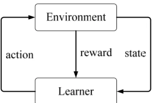
Figure 3.1 : Block diagram of a learning system
3.1 Fuzzy Q-Learning Algorithm
c3 1
First we give a brief introduction of the fuzzy Q-learning (FQL) algorithm [15],
[16], [17], [18].
As shown in Fig 3.1, a general learning system consists of five elements. The
learner will interact with the environment and make a decision according to the state.
After the decided action is applied, some reward resulting from the acting will be
feedback to the learner and be used to justify the decision policy.
The basic idea of the reinforcement learning is to learn an optimal policy which
can choose the best action in order to maximize (minimize) the accumulation of
rewards (costs) induced by the selected action each time. The expectation of the
accumulation, called Q-function, is related to the action, denoted by a, as well as the
state of system, denoted by x, which is defined as
(
0 0)
(
)
0 0 0 , n ( ), ( ) (0) , (0) , n Q x a E γ r x n a n x x a a ∞ = ⎧ ⎫ = ⎨ = = ⎬ ⎩∑
⎭ (3-1)where r is the reward, also called reinforcement signal, γ is the discount factor , n in ( )x n or ( )a n is the index of the episode of the system state or action and
{}
E ⋅ is the expectation operation. The output of Q-function, called Q-value, is the
from now on and this expectation value will be effected by the selected action a0
under state x0 at current decision episode n=0. The optimal action, denoted by *
a ,
can be obtained by:
*
0
arg max ( , ).
a
a = Q x a (3-2)
However, the system state in the future, ( ) for x n n> , and the expectation value of 0
r are usually unavailable in the real world. It is hard to build the relation among action a, system state x and expected value of feedback r . Watkins and Dayan
[14] proposed a recursive method, called Q-learning algorithm, to solve above
problems and obtain an the optimal Q function, denoted by Q . The rule of each step *
of the learning method, resulting from mathematical inferring of Eq. (3-1), can be
given by [14]
[
1 ( , ) ( ( ), ( )) ( , ) max[ ( ( 1), )] ( ( ), ( )) , for ( , ) ( ( ), ( )) , ( , ), for ( , ) ( ( ), ( )). n n n n n a n Q x a r x n a n Q x a Q x n a Q x n a n x a x n a n Q x a x a x n a n η γ + ⎧ + ⎪⎪ ⎤ =⎨ + + − ⎦ = ⎪ ≠ ⎪⎩ (3-3)where ( , )Q x a is the transient function for n Q at episode * n, and ηn is the learning rate at the n-th episode, ηn∈[0,1]. It is assumed that the next system state x n( + is 1) available. At episode n+1, feedback reward ( ( ), ( ))r x n a n caused by the last action is
used to update Q x a to get a new function n( , ) Qn+1( , )x a . It should be noticed that only the state-action pair ( , )x a which occurrs in the just past episode will have
information to correct its Q-value in this episode. After updating, we can use a more
accurate Q-function approximation and the policy in Eq. (3-2) to select the action.
The fuzzy Q-learning (FQL) algorithm can be regarded as the Q-learning
combination scheme can be observed from the general form of fuzzy inference system
(FIS) rules:
Rule : if ( ) is j X n Sj, then ak with q S an( j, k), 1≤ ≤k K. (3-4)
where X n( )=
[
x n1( ),...,xH( )n]
is the vector of input linguistic variables, H is thenumber of input variables, and q S an( j, k)is the Q-value for the state-action pair (S aj, k)at the episode n. Denote S=
{
Sj,j=1,...,J}
as the set of state vectors. The uncertain input vector X n will belong to each ( ) S with different intensity jdepending on the membership function of input variables. A=
{
a kk, =1,...,K}
is the set of action candidate. For simplification, we assume each S containing a rule. jThen we will get J different Q-values qn
(
S a nj, ( ) ,)
j=1,...,J for each pair ( ( ),X n ak),k=1,...,K and can infer Jconsequences from these J rules separately. In this thesis, the so called select-max strategy is adopted for each rule to choosethe most suitable action:
* A ( ) arg max ( , ) . k j n j k a a n q S a ∈ = (3-5)
Then these consequences a n*j( ), j=1,...,J will be gathered to infer the global optimal action, denoted by *
( ) a n * , 1 * , 1 ( ) ( ) , J j n j j J j n j a n a n μ μ = = × =
∑
∑
(3-6)the membership function of each input variable.
As in traditional Q-learning algorithm, q S an( j, k) is a transient value at time n and will be updated after reward is replied. The Q-function updating operation to get
new qn+1(S a nj, *( )),j=1,...,J is given by * * * 1( , ( )) ( , ( )) ( , ( )), for 1 , n j n j n n j q + S a n =q S a n + × Δη q S a n ≤ ≤j J (3-7) and
(
)
(
)
(
)
{
}
* , * * * , 1 ( , ( )) , ( ) ( 1), ( 1) ( ), ( ) . n j j n j n n J i n i q S a n r S a n Q X n a n Q X n a n μ γ μ = Δ = × + × + + −∑
(3-8)Here Qn
(
X n a n( ), *( ))
, the Q-value for state-action pair ( ( ),X n a n*( )), is the weighted summation of the J Q-values q S a nn( j, *j( )), j=1,...,Jby using the rule intensity μj n, of ( )X n :(
)
(
)
* , 1 * , 1 , ( ) ( ), ( ) . J j n n j j j n J j n j q S a n Q X n a n μ μ = = ⎡ × ⎤ ⎣ ⎦ =∑
∑
(3-9) * ( ( 1), ( 1)) nQ X n+ a n+ is the next-stage optimal global Q-value. Since the next stage Q-values qn+1(S aj, k), j=1,..., ,J k=1,...,K are not available, Q X n*n( ( +1), (a n+1)) will be calculated by q S an( j, k), j=1,..., ,J k =1,...,K which is defined as
(
)
(
)
* , 1 1 * , 1 1 , ( ) ( 1), ( 1) . J j n n j j j n J j n j q S a n Q X n a n μ μ + = + = ⎡ × ⎤ ⎣ ⎦ + + =∑
∑
(3-10)Step 1: Initialize qj n, (S aj, k)for all pair (S aj, k),k=1,...,K j, =1,...,J. Step 2: Observe the input linguistic vector X n . ( )
Step 3: Using Eq. (3-5) to find *
( ), 1,...,
j
a n j= J
Step 4: Use Eq. (3-6) to infer the global optimal action a n and then *( ) imply it to the system.
Step 5: Compute the reinforcement signal *
( j, ( ))
r S a n and measureX n( + 1) Step 6: Update *
, ( , ( ))
j n j
q S a n for all j using Eq. (3-7), (3-8), (3-9), (3-10).
Step 7: Return to step 2 and repeat.
In summary, the procedure of the FQL algorithm step is list as following:
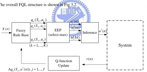
The overall FQL structure is shown in Fig 3.2.
Fuzzy Rule Base 1 ( , ) n k q S a ( , ) n J k q S a Inference ( ) X n q S an( 2, k) EEP (select-max) * 1( ) a n * 2( ) a n * ( ) J a n * ( ) a n System Q-function Update * ( , ( )), 1,.., n j q S a n j J Δ = ( ) r n (k=1,...,K)
Figure 3.2 : The overall structure of FQL
3.2 Input and Output Linguistic Variables
c3 2The structure of the FQL algorithm was described in section 3.1. In this section,
HARQ scheme (FQL-HARQ).
At decision episode n, the FQL-HARQ scheme chooses two system measures
as input linguistic variables. First is a short-term block error rate (BLER) performance
indicator, which is denoted as BLER n and defined as the failure times in the last N ( ) packets from the (n-N)-th to the (n-1)th transmission over N. The other one is
( )
CQI n , the channel quality indicator received at episode n. The values of CQI n ( ) will be a discrete number and at the range of [0, 30] since the reporting information is
composed of 5 bits in the HSDPA scheme. These two variables will be the fuzzy input
to help infer the most suitable modulation order and coding rate scheme (MCS)
decision. That is, we have X n( )=
{
BLER n CQI n( ), ( )}
in the FQL-HARQ system. In this thesis, we assume two kinds of modulation order, QPSK and 16 QAM,and five kinds of coding rate, 1 1, , , 2 3 and 4
3 2 3 4 5, resulting in totally 10 kinds of modulation and coding pairs, to be chosen. The MCS pair pool, which is shown in
Table 3-1, is the set for the output linguistic variable a mentioned in section 3.1. *n
And we number these MCSs from 1 to 10 depending on the degree of BLER
performance. Under the same channel condition, MCS with lower BLER will have
smaller number.
The fuzzy term sets for the two fuzzy input linguist variables, BLER n and ( ) ( )
CQI n are defined as T BLER n
(
( ))
= {Green, Yellow, Red} = {G, Y, R} where(
( ))
T CQI n ={Level 1, Level 2, Level 3, Level 4, Level 5, Level 6, Level 7, Level 8,
Level 9, Level 10} ={L1, L2, L3, L4, L5, L6, L7, L8, L9, L10}, respectively. Terms
in T BLER n
(
( ))
are used to describe the degree of the BLER performance. Based on the QoS requirement of BLER, denoted by BLER , “Green”, here, means the BLER *2/3 16QAM 8 2/3 QPSK 4 Coding rate Modulation order MCS number 4/5 16QAM 10 3/4 16QAM 9 4/5 QPSK 7 3/4 QPSK 6 1/2 16QAM 5 1/3 16QAM 3 1/2 QPSK 2 1/3 QPSK 1 2/3 16QAM 8 2/3 QPSK 4 Coding rate Modulation order MCS number 4/5 16QAM 10 3/4 16QAM 9 4/5 QPSK 7 3/4 QPSK 6 1/2 16QAM 5 1/3 16QAM 3 1/2 QPSK 2 1/3 QPSK 1
Table 3-1: the action pool and numbers of actions
performance is “safe” while “Yellow” is “general” and “Red” is “violation”. On the
other hand, terms in T CQI n
(
( ))
stand for the judgment of channel quality indication and are designed with the ten levels, which is related to the 10 kinds of MCS adoptedin the system. Each level will be at the SINR regions supporting BLER* when using its corresponding MCS. The membership functions for these fuzzy terms, which can
indicate the intensity the input variables belong to itself fuzzy labels are shown in the
following.
The membership is defined by the designer with pre-knowledge of the system.
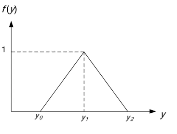
To illustrate the membership function, first we define a triangle function f( )⋅ which is expressed as
(
)
1 0 1 1 0 0 1 2 1 1 2 1 0 1 for ; , , 1 for 0 otherwise y y y y y y y f y y y y y y y y y y y − ⎧ + ≤ ≤ ⎪ − ⎪⎪ =⎨ + − ≤ ≤ ⎪ − ⎪ ⎪⎩ (3-11)where y0 , y1, y2 in f( )⋅ is the left edge, center, right edge of the triangular
Figure 3.3 : Definition for function f( )⋅
Then we define a trapezoid shape function g( )⋅ which is expressed as
(
)
1 1 2 2 1 2 3 1 2 3 4 3 3 4 4 3 , for 1 , for ; , , , , , for 0 , otherwise x x x x x x x x x x g x x x x x x x x x x x x − ⎧ ≤ ≤ ⎪ − ⎪ ≤ ≤ ⎪ = ⎨ − ⎪ ≤ ≤ ⎪ − ⎪ ⎩ (3-12)where x1 ,x2, x3, x4 in ( )g ⋅ are the left edge, center-right, center-left and right
edge of the trapezoid respectively. The basis shape of this function is shown in
Fig 3.4. 1 1 x x2 x3 x4 ( ) g x x
Figure 3.4 : Definition for function g( )⋅
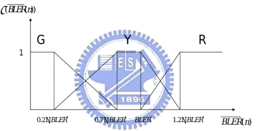
The membership function of BLER n( ) , denoted by μ
(
BLER n( ))
, is constituted by the membership functions for the terms, G, Y, and R of T BLER n(
( ))
,denoted by μG
(
BLER n( ))
, μY(
BLER n( ))
, μR(
BLER n( ))
, respectively which can be given by(
( )) (
( ); - , 0, ,)
, G BLER n g BLER n b a μ = ∞ (3-13)(
) (
*)
( ) ( ); , , , ,Y BLER n g BLER n b a BLER c
μ = (3-14)
(
) (
*)
( ) ( ); , , 1, .
R BLER n g BLER n BLER c
μ = ∞ (3-15)
The figure of μ
(
BLER n( ))
is shown in Fig 3.5.( ) BLER n * BLER 1.2 BLER× *
G
Y
R
1 (BLER n( )) μ * 0.7 BLER× * 0.2 BLER×Figure 3.5 : The membership function of BLER n ( )
The membership function μ
(
CQI n( ))
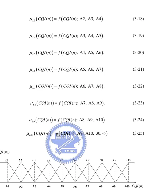
is defined and shown in Fig 3.6. As mentioned, Ai is set to be the required SINR to maintain*
BLER while using the i-th modulation and coding scheme (MCS ii, =1,...,10). Again we expressμ(CQI n( )), which is constituted by the membership functions for the terms, L1,…,L10, of
( )
CQI n , denoted by μL1
(
CQI n( ))
,…, μL10(
CQI n( ))
, as(
)
(
)
1 ( ) ( ); - , 0, A1, A2 . L CQI n g CQI n μ = ∞ (3-16)(
)
(
)
2 ( ) ( ); A1, A2, A3 . L CQI n f CQI n μ = (3-17)(
)
(
)
3 ( ) ( ); A2, A3, A4 . L CQI n f CQI n μ = (3-18)(
)
(
)
4 ( ) ( ); A3, A4, A5 . L CQI n f CQI n μ = (3-19)(
)
(
)
5 ( ) ( ); A4, A5, A6 . L CQI n f CQI n μ = (3-20)(
)
(
)
6 ( ) ( ); A5, A6, A7 . L CQI n f CQI n μ = (3-21)(
)
(
)
7 ( ) ( ); A6, A7, A8 . L CQI n f CQI n μ = (3-22)(
)
(
)
8 ( ) ( ); A7, A8, A9 . L CQI n f CQI n μ = (3-23)(
)
(
)
9 ( ) ( ); A8, A9, A10
L CQI n f CQI n μ = (3-24)
(
)
(
)
10 ( ) ( ); A9, A10, 30, L CQI n g CQI n μ = ∞ (3-25) (CQI n( )) μ ( ) CQI n 1 L L2 L3 L4 L5 L6 L7 L8 L9 L10Figure 3.6 : The membership function of CQI n( )
3.3 Design of the FQL Rules Base
c3 3
In section 3.2, we have selected the input and output linguistic variables as well
as defined the membership function of input variables for the fuzzy interface. In this
section, we will design the fuzzy rule base, which is consisted of the if-then rules and
rule.
The rule form of the FQL is shown in Eq. (3-4). We need to design the
reinforcement signal for each rule to update the q-value of each action and accomplish
the Q-learning operation. Design of the fuzzy rules will be based on the concept that
the choice of MCS will be more aggressive if better BLER n performance, and on ( ) the other hand, is more conservative if worse BLER n . The decision is mainly ( ) counted on BLER n , while ( ) CQI n will be used to determine the selection base so ( ) as to accelerate the learning procedure. Therefore we divide the rules into three parts
based on the 3 fuzzy terms, Green, Yellow and Red. Rules in the same parts will have
the same reinforcement signal. The details of each part are described in the following.
Part 1: if
BLER n( )is Green, and
CQI n( )is Level
m, then
k
MCS
with
qn(
(BLER n( ) is Green ,CQI n( ) is m),MCSk)
,k >mThere are 10 rules (1≤ ≤m 10)in part 1. In this part, BLER n is considered to ( ) be in a safe region where BLER n is much smaller than ( ) *
BLER . The main goal is to maximize the throughput. To be more aggressive, only MCSk with k > will be m
considered. The amount of carrying information and whether the signal could be
successfully decoded before dropping will be focused. Thus the reinforcement signal
is designed as , if succesful transmission, 10, if failure transmission, k k k MCS MCS rd R R R r ⎧ ⎪ + = ⎨ ⎪ − ⎩ (3-26) where k MCS
k
rd
R is the required redundancy bits ,contained in the initial transmission and the retransmission, for the successful transmission We will update the q-value after the
transmission of the packet is completed. It can be expected that higher achievable data
rate after transmission will get larger reward feedback. If the transmission fails to be
decoded after 3 retransmissions, the block will be dropped and we will give a severe
punishment, r= -10 at such condition.
Part 2: if
BLER n( )is Yellow, and
CQI n( )is Level
m, then
k
MCS
with
qn(
(BLER n( ) is Yellow ,CQI n( ) is m),MCSk)
,m− ≤ ≤ +1 k m 1There are 10 rules (1≤ ≤m 10)in part 2. Yellow BLER n means that the ( ) BLER performance is around the requirement. It will be better to keep BLER still in a
safe range. Hence we will choose the MCS which has the BLER nearest to BLER *
under CQI n while containing the most information.( ) MCS ,k k = −m 1, , 1m m+ ,
will be the considered action candidates. The reinforcement signal in this part is set as
* , k MCS MCS R r R σ = × (3-27)
where RMCS* is the number of information bits if 16 QAM modulation order and coding rate 4
5, and σ is a scalar, which is 1
8 if successful decoding after initial
transmission and − if failed. Here the degree of reward is normalized by 1 RMCS* to be proportional to the amount of information data.
σ is a weighting factor according to the BLER requirement 0.1. Since it means the occurrence possibility of success and failure transmission has the ratio equal to 9,
ratio 1
9. For the reason to be more aggressive, we increase the ration up to 1
8. And if the transmission is dropped, we will give a severe punishment r=-10.
Part 3: if
BLER n( )is Red, and
CQI n( )is Level
m, then
k
MCS
with
qn(
(BLER n( ) is Red ,CQI n( ) is m),MCSk)
,k<mThere are 10 rules (1≤ ≤m 10)in this part. Red BLER n represents BLER ( ) requirement violation. It will be better to take action to recover from this situation.
The action decision should be more conservative, thus MCS kk, < will be chosen. m
The reinforcement signal is set as
* , if successful decoding after initial transmission.
1, if failed decoding after initial transmission. -10, if transmission is dropped. MCS MCS R R r ⎧ ⎪⎪ = ⎨− ⎪ ⎪⎩ (3-28)
Only when the packet is successfully decoded in the initial transmission, the system
will be rewarded. The degree of reward is proportional to the amount of information
bits. If the initial transmission failed, the system will be given a severe punished
r=-10.
There are ten rules contained in each part separately. The intensity of the 30
rules j , j=1,..., 30 will be inferred from the membership functions of BLER n and ( ) ( )
CQI n by a max-product operation, which can be expressed as
(
)
(
)
, ( ( )) ( ( )), where ( ) and ( ) .
j n α BLER n β CQI n T BLER n T CQI n
μ =μ ×μ α∈ β∈
(3-29)
Here j is the number of rule respect to the case that BLER n is ( ) α and CQI n is ( )
pair of the input variable fuzzy terms
(
α β,)
, ∀ ∈α TBLER n( ) and ∀ ∈β TCQI n( ) whilej represent the index number of the fuzzy term pair.
Every TTI, the system state pair (BLER n CQI n( ), ( ))will be inputted and then the local optimal actions a*j(n), 1,...,j= J will be inferred by select-max EEP, Eq (3-5), as well as the Q-learning algorithm based on above fuzzy rules separately. Here a n*j( )
represented the number of selected action. Then these local optimal actions
*
(n), 1,...,
j
a j= J will be used as well as μj n, to get the global optimal action a n*( ) by Eq. (3-6). However *
( )
a n would be continuous while the output should be discrete in our application. Then we will use some method to map the continuous
result a*n to discrete output action a*n d, . The continuous result *
( )
a n will be quantized by following principle:
* * * * * * * ( ) , with probability ( ) ( ) ( ) , ( ) , with probability ( ) ( ) d a n a n a n a n a n a n a n ⎧⎡ ⎤ −⎢ ⎥ ⎪⎢ ⎥ ⎣ ⎦ = ⎨ ⎢ ⎥ −⎡ ⎤ ⎪⎣ ⎦ ⎢ ⎥ ⎩ (3-30) where * * * * * * * *
( ) , ( ) are the integer at [1,10] such that ( ) 1 ( ) ( ) . ( ) ( ) ( ) 1 a n a n a n a n a n a n a n a n ⎡ ⎤ ⎢ ⎥ ⎢ ⎥ ⎣ ⎦ ⎧ − <⎢ ⎥≤ ⎪ ⎣ ⎦ ⎨ ⎡ ⎤ < ≤ + ⎪ ⎢ ⎥ ⎩ (3-31) * ( ) d
a n is the final action.
After the base station use the decision MCS to transmit and the transmission is
finished such that the reinforcement signal of each part is available, operations in Eq.
chapter 4
Chapter 4
Simulation Results and Discussions
4.1 System Environment and Parameters
c4 1
In our simulation, we consider a hexagonal grid cell structure. There are 19 base
stations (BS) in the multi-cell system to consider 2-tier neighboring cell interference.
For a HSDPA user, we assume that the HS-DSCH is allocated at maximum up to 80%
of the total power of a BS. In this thesis, we define HSDPA service power ratio
(HSPR) to represent the ratio of transmission power on the HS-DSCH for the HSDPA
user to the total transmission power at BS side. The residual power except for HSDPA
service will be used for other service and control channels within same cell. The
interference from other cell is fixed. Here we use HSPR, which controls not only the
amount of HSDPA transmission power but also the interference from self cell, as
condition variable to observe the system performance.
In the simulation, we will observe and compare the system performance of both
circumstances with and without CQI delay consideration. The CQI delay is set to be
6ms if considered. To evaluate the maximal achievable throughput, we assume that
the users always have data to be transmitted to. The channel model is described in
detailed simulation environment parameters are shown in Table 4-1.
Table 4-1 : Simulation parameters
Parameter Assumption Cellular layout Hexagonal grid, 19 sites, 1000m cell radius
Path loss model
(
ξ( )
r)
128.1 + 37.6log10(r)r is the base station separation in kilometers Decorrelation length ( dcor) 30m
L
σ 8.0
Mobility assignment 0 km/hr to 120 km/hr, random distribution Carrier frequency 2.0 GHz
Channel bandwidth 5.0 MHz
Chip-rate 3.84 Mcps
Spreading factor 16 Thermal noise density -174 dBm/Hz
TTI length 2 ms
Forgetting factor (γ) 0.1 Learning rate (η) 0.9
N 50 BS total Tx power Up to 44 dBm
Power for HSDPA data transmission
Maximum of 80% of total maximum available transmission power
ACK/NACK delay 6ms
4.2 Conventional Schemes
c4 2In the simulation, we will compare the proposed FQL-HARQ scheme with some
other conventional schemes. According to [10], we need to choose a suitable MCS at
initial transmission in the HARQ process to maintain the BLER requirement 0.1.
Three conventional schemes are described in the following:
¾ Fixed threshold selection [10] :
Based on the pre-known BLER performance, the fixed threshold selection
(FTS) scheme sets fixed SINR threshold for each MCS. The threshold is the
required SINR that the MCS has BLER equal to the requirement 0.1. At each
TTI, FTS will choose the MCS whose corresponding threshold is just under and
closest to the measured SINR.
¾ Adaptive threshold selection (Adaptive control of link adaptation [11] ) :
Compared with FTS, the adaptive threshold selection (ATS) scheme
improves the performance of users with high mobility. ATS sets threshold for
every MCS, too. Moreover, after a transmission is completed, the thresholds
which are close to the SINR of last transmission will be updated based on the
block decoding result. The thresholds will be increased if failed initial
transmission and be deceased if succeeded. The ratio of increasing and
decreasing step is set to be
* * 1 BLER BLER − . ¾ Q-learning based HARQ (QL-HARQ) [13] :
Without any pre-knowledge of BLER performance of each MCS,
QL-HAQR uses the Q-learning algorithm to learn an optimal policy in both link
designed to be the normalized difference square of received SINR and required
SINR for maintaining BLER=0.1. After learning, QL-HARQ will choose a MCS
whose required SINR to maintain BLER=0.1 is closest to the received SINR.
In next section, we will show the performance of the FQL-HARQ scheme and the
traditional schemes versus HSPR with and without CQI delay. Besides, we will also
display the simulation results of these schemes versus different UE mobility with
fixed power allocation, and discuss about it.
4.3 Simulation Results and Discussions
c4 3Fig 4.1(a) and Fig 4.1(b) show the transmission block error rate versus HSPR
without and with 6ms CQI delay considering for the proposed FQL-HARQ scheme
and three comparative schemes. It can be seen in Fig 4.1(a) that when more than 70%
BS transmission power is allocated for HSDPA service, all schemes can perform MCS
adaptation under satisfying the BLER requirement without CQI delay. However,
when the CQI delay is considered, FTS and QL-HARQ will violate the BLER
requirement even with HSPR up to 80% as shown in Fig 4.1(b). The mobility of UEs
in the simulation is uniformly distributed at the range from 0 to 120 km/hr. Motion of
UEs will incur not only the Doppler Effect but the higher channel variance, and then
affect the accuracy of channel condition information for MCS determination. After 6
ms, the actual transmission channel condition may be much different from the
information used for determination. Compare the results of Fig 4.1(a) and Fig 4.1(b),
we can find that FTS and QL-HARQ are not flexible enough to accommodate to
imperfect CQI report. The MCS determination may not suitable to the transmission
30 35 40 45 50 55 60 65 70 75 80 0.02 0.04 0.06 0.08 0.1 0.12 0.14 0.16 0.18 0.2 HSPR (%) BL ER FQL QL ATS FTS
Figure 4.1(a): The BLER comparison versus HSPR without CQI delay.
30 35 40 45 50 55 60 65 70 75 80 0.02 0.04 0.06 0.08 0.1 0.12 0.14 0.16 0.18 0.2 HSPR (%) BL ER FQL QL ATS FTS
Figure 4.1(b): The BLER comparison versus HSPR with CQI delay.
On the other hand, ATS, the modified scheme for FTS, and our proposed scheme,
FQL-HARQ are more sensitive to the channel variance and able to modify the MCS
detection policy based on the past transmission result adaptively, so they can make the
BLER requirement as shown in Fig 4.1(a) and Fig 4.1(b). If failure initial
transmission occurs too frequently, ATS and FQL-HARQ will decrease the rating of
CQI and justify the decision rule to be conservative. So they can maintain the BLER
requirement.
It can be observed that BLER of FQL-HARQ will violate the requirement a little
when HSPR is smaller than 35% at both circumstances with and without CQI delay
consideration. This is because that at low SNR, there are fewer MCSs for selection as
shown in Fig 4.2. Since the SNR gap between the considerable MCSs at low SNR is
larger, the idea of FQL-HARQ to choosing more aggressive MCS if better short term
BLER (SBLER) than requirement will result in too aggressive MCS decision. When
at low HSPR, UE may face bad channel condition (low SNR) more frequently, and
hence too much forward MCS selection will accumulate. So FQL-HARQ is going to
violate the requirement at HSPR smaller than 35%. This can be resolved by increasing
N, the window size of SBLER. If we increase N to 500, FQL-HARQ can maintain the
requirement even with HSPR below 40% yet will decrease the throughput of the
system.
For the same reason, it can be seen in Fig 4.1(a) and Fig 4.1 (b) that BLER of
QL-HARQ will be affected by low HSPR more intensely. When the power allocated
for HSDPA user is less than 65% BS transmission power, the BLER performance of
QL-HARQ will get worse and violate the requirement severely. As mentioned in
section 4.2, the decision of QL-HARQ will be the MCS with required SINR
maintaining 0.1 BLER closest to the reporting CQI but neglecting whether the former
-4 -2 0 2 4 6 8 10 0 0.1 0.2 0.3 0.4 0.5 0.6 0.7 0.8 0.9 1 SNR (dB) BL ER MCS1 MCS2 MCS3 MCS4 MCS5 MCS6 MCS7 MCS8 MCS9 MCS10
Figure 4.2 : The BLER of turbo code of each MCS versus SNR under AWGN.
considerable MCSs at low SNR as shown in Fig 4.2 and then result in too high BLER.
Compare FQL-HARQ and QL-HARQ: on account of considering the performance
and following HARQ process in reinforcement signal after using more aggressive
MCS, FQL-HARQ can avoid the BLER violation at low HSPR more effectively than
QL-HARQ does.
It can also be found in Fig 4.1 (a) that FTS and ATS have almost the same
performance when CQI delay is not considerable, unless at low HSPR. ATS gets a
little higher BLER than that of FTS at low HSPR. This is also due to the bigger SINR
gap within MCS at low SNR and the thresholds updating range of ATS.
Fig 4.3(a) and Fig 4.3(b) show the system throughput for the four schemes in
case of without and with 6ms CQI delay. Definitely it can be seen that as HSPR
increases, the throughput of all schemes increases in both cases, too, and all schemes
has better system throughput with perfect CQI than that of itself with CQI delay,
information can result in higher system throughput since it is helpful to decrease the
probability of executing wrong threshold adaptation. We can also find that FTS, the
only non-adaptive scheme, keep the maximal throughput among the four schemes. By
using perfect CQI, the adaptive operation of the other schemes will inference the
instant MCS decision and make it be too conservative when channel condition is
good.
Then compare the performance of FQL-HARQ and ATS, which are the only two
schemes able to make the requirement when CQI delay is considered. It can be seen in
Fig 4.1(b) that ATS keeps a lower BLER than FQL-HARQ does. This is for the reason
that ATS tune the selection threshold based on current ACK/NACK result directly and
immediately, while FQL-HARQ tunes the selection policy based on a long term
measure, BLER n , more sophisticatedly and then results in more slowly updating ( ) process than that of ATS. Nevertheless it is can be seen in Fig 4.3(b) that FQL-HARQ
reaches a much higher throughput than ATS does. This is because that only BLER
performance is considered and affects the threshold updating process for ATS scheme.
On the other hand, as mentioned in Chapter 3, the MCS decision of FQL-HARQ is
inferred from the fuzzy rules which are justified by reinforcement signals. Rule base
is designed and separated to different parts according to the BLER requirement while
the reinforcement signals are set so as to reward MCS with higher throughput. Since
both BLER maintaining and throughput maximizing are considered in FQL-HARQ,
the throughput can be enlarged by a more aggressive but safe MCS determination.
Due to the too immediately threshold tuning, the selection policy of ATS may oscillate
30 35 40 45 50 55 60 65 70 75 80 0.3 0.35 0.4 0.45 0.5 0.55 0.6 0.65 HSPR (%) T hr o ugh put ( M bp s ) FQL QL ATS FTS
Figure 4.3(a): The system throughput versus HSPR without CQI delay
30 35 40 45 50 55 60 65 70 75 80 0.35 0.4 0.45 0.5 0.55 0.6 0.65 0.7 HSPR (%) T hr o ugh put ( M bp s ) FQL QL ATS FTS
Figure 4.3(b): The system throughput versus HSPR with CQI delay. Figure 4. 3f
30 35 40 45 50 55 60 65 70 75 80 0.06 0.07 0.08 0.09 0.1 0.11 0.12 HSPR (%) Dr o p p in g Ra te FQL QL ATS FTS
Figure 4.4 : The dropping rate comparison versus HSPR with 6ms CQI delay
Fig 4.4 depicts the dropping rate versus HSPR with 6ms CQI delay. In the
simulation, every transmission block has at most three times of retransmission. If the
block fails to be decoded after the third retransmission, the block will be dropped. It
can be seen obviously that a more conservative initial transmission MCS selection,
which has smaller initial BLER, can result in lower retransmission dropping rate. Low
dropping rate can decrease the signaling cost, however may reduce the system
throughput by using too conservative MCS. As shown in Fig 4.3(b) and Fig 4.4,
FQL-HARQ can keep a more balance performance in the trade off between dropping
rate and throughput maximizing than the other three schemes. It can also be found in
Fig 4.4 that QL-HARQ is more sensitive to HSPR than the others. As mentioned, this
is because of the MCS BLER distribution versus SNR shown in Fig 4.2. At high SNR,
there are more MCSs for selection and then smaller SNR gap between the
considerable MCSs, so the QL-HARQ can execute a more accurate learning process.
increases while the BLER of both schemes decrease as shown in Fig 4.1(b). This is
because that the SNR gap between considerable MCS at high SNR is smaller than that
at low SNR. The considered coding rate schemes are 4, , , 3 2 1 , 1
5 4 3 2 3 of the order with SNR performance. If the decoding of the transmission block fails, appending
redundancy bits will be transmitted to the user so that the block will have the next
stage coding rate after retransmission. When the SNR gap of MCS is small, which
means the BLER performance will improve a little after retransmission, the decoding
failure rate will still be high after three retransmissions. So the dropping rate of FTS
and ATS will arise little at high HSPR. On the other hand, since the dropping
condition is considered in FQL-HARQ, which the Q values of fuzzy rules will be
updated by a severe punishment signal, the dropping rate can keep stable as HSPR
Fig 4.5(a) and 4.5(b) show the BLER performance and system throughput of the
four schemes versus different user mobility. In the simulation, BS allocate 80% of the
total transmission power for the HSDPA user, and CQI has 6ms delay. We can see that
all schemes has better performance when the UE is immotility than that of itself when
the UE with mobility. Besides, FTS, the only scheme with fixed selection policy, has
better BLER and throughput performance than the other three adaptive schemes when
the UE is at low speed and with low cannel condition variance. However FTS has the
worst BLER requirement violation when the UE at mobility higher than 45 km/hr
among all schemes. This is due to the channel information inaccuracy resulting from
CQI delay and Doppler Effect. On the other hand, when the variance of CQI
inaccuracy is small, i.e. UE at low mobility, schemes with too rapidly channel
adaptation, i.e. ATS, will choose too conservative MCS and result in non-effective
system throughput. Again we can find that FQL-HARQ can reach the maximal system
throughput among the schemes which can maintain the BLER requirement at the
same time.
Surprisingly, we can also find in Fig 4.5(a) and Fig 4.5(b) that when the mobility
is beyond 30 km/hr and get higher, the BLER will decrease and the system throughput
will increase a little for all schemes on the contrary. This is because when the mobility
of the UE is higher than 30 km/hr, the effect of channel variance and CQI inaccuracy
are almost the same. Instead, the effect of path loss will dominate the system
throughput. A traveling UE may either move toward the BS and then get better
channel condition or move apart the BS and then get worse path loss effect. Fig 4.6 is
the path loss effect versus the distance in km between BS and UE. In reality, a mobile
user in the cell should have moving direction with uniform probability distribution. It
can be observed from the path loss curve in Fig 4.6 that with the same movement, the
0 20 40 60 80 100 120 0.02 0.04 0.06 0.08 0.1 0.12 0.14 Mobility (km/hr) BL ER FQL QL ATS FTS
Figure 4.5(a): The BLER versus different mobility of UE with CQI delay
0 20 40 60 80 100 120 0.35 0.4 0.45 0.5 0.55 0.6 0.65 0.7 Mobility (km/hr) T hr o ugh put ( M bp s ) FQL QL ATS FTS