在蜂巢式網路結合道路拓樸的架構下提供強健性的允入控制機制

全文

(1)國立交通大學電信工程學系碩士論文在蜂巢式網路結合道路拓樸的架構下提供強健性的允入控制機制 A Robust Call Admission Control in Road Topology Based Cellular Networks. 研究生：陳郁媛指導教授：廖維國教授. 中華民國九十七年七月.

(2) 在蜂巢式網路結合道路拓樸的架構下提供強健性的允入控制機制 A Robust Call Admission Control in Road Topology Based Cellular Networks. 研究生：陳郁媛指導教授：廖維國博士. 國立交通大學電信工程學系碩士班碩士論文. A Thesis Submitted to the Department of Communication Engineering College of Electrical and Computer Engineering National Chiao Tung University in Partial Fulfillment of the Requirements for the Degree of Master of Science In Communication Engineering Jul. 2008 Hsinchu, Taiwan, Republic of China. 中華民國九十七年七月. ii.

(3) 在蜂巢式網路結合道路拓樸的架構下提供強健性的允入控制機制研究生：陳郁媛. 指導教授：廖維國博士. 國立交通大學電信工程學系碩士班. 中文摘要在無線通訊中，由於每個細胞基地台所配置的通道數目有限，因此如何使通道達到最有效的利用成為一個重要的問題。在此篇論文中，我們研究在蜂巢式網路結合道路拓樸的架構下，將環繞於基礎細胞(base cell)周圍鄰接細胞(adjacent cell)的通話資訊與通話位置列入考慮，利用這些資訊完成允入控制機制。對於每個細胞，我們使用二維狀態的馬可夫鏈(Markov chain)來模擬此系統，第一維代表基礎細胞使用通道的狀態，第二維是代表鄰接細胞使用通道的狀態。對於以最小化新連線的阻斷率(new call blocking probability)和連線交遞的失敗率(handoff dropping probability) 為目標函數的問題，可以使用馬可夫決策過程 (Markov Decision Process)來描述。在模型中，我們利用了一些變數來描述整個系統，這些變數是非線性、難以預測的，然而模型所能展現效能的優劣與這些變數估測的精準度息息相關。為了避免所取得的模型與真實系統相差甚遠，變數的估測是我們成為我們關注的主題。我們提出利用 Cost Match Update(CMU)來調整參數，使參數估測能較接近實際狀態。經由實驗結果，我們證實了使用 CMU 確實可以使模型的效能更加提升。. i.

(4) A Robust Call Admission Control in Road Topology Based Cellular Networks Student: Yu-Yuan Chen. Advisor: Dr. Wei-Kuo Liao. Department of Communication Engineering National Chiao Tung University. Abstract In wireless communication, the number of channels allocate to each cell is limited, so how to use channel efficiently is an important topic. In our thesis, we study the call admission control in road topology based cellular networks, and we take the mobile communication information and position in adjacent cells into consideration. For each cell, we formulate the system by Markov Chain with two-dimensional states where the first dimension represents the base cell’s state and the second dimension stands for the adjacent cells’ state. The problem of minimizing a linear objective function of new call blocking rate and handoff call dropping rate can be formulated as a Markov Decision Process. In our model, we use several parameters to model our system, and these parameters are non-linear and difficult to measure and predict. How the model performs depending on whether these parameters are estimated precisely. In order to avoid our model very different from the reality, we use Cost Match Update (CMU) rule to help us to estimate parameter. In simulation result, it shows our proposed scheme has lower average cost than others.. ii.

(5) Acknowledgement. 在研究所求學的過程中，非常感謝廖維國老師在課業上給我的指導與教誨，感謝老師在我迷惘與遇到困難時指引我正確的研究方向，才能使本篇論文順利完成。此外，老師於為人處世也給予我許多的看法與態度，使我在和老師學習的這幾年受益良多。感謝我最親愛的家人，在研究生涯裡給我無限的溫暖與鼓勵，有你們的照顧與支持才有現在的我。感謝實驗室的所有成員，在和大家的相處中，讓我單調的研究生生活增添了許多顏色。另外也謝謝昔日的同窗好友們，由於你們的督促與鼓舞，使我能不斷的努力向前。最後要感謝的是我的室友們，和你們相處的每一天都非常的開心有趣，謝謝你們這幾年來宛如家人般的關心與陪伴。. iii.

(6) Table of Contents Abstract (in Chinese). ……………………………………………………………....i. Abstract (in English). ………………………………………………………………ii. Acknowledgement…………………………………………………………………...iii Table of Contents…………………………………………………………….………iv List of Figures……………………………………………………………….……….vi List of Tables………………………………………………………………………...vii Chapter 1. Introduction………………………………………………………………..1 Chapter 2. Related Works……………………………………………………………..4 2.1 Wireless Cellular Networks…………………………………………………..4 2.2 Minimizing a Linear Objective Function (MINOBJ) ………………………..5 2.3 Markov Decision Process…………………………………………………….6 2.3.1 State and Transition………………..………………………………….6 2.3.2 Transition Probability……………...………………………………….6 2.3.3 Rewards……………………………………………………………….6 2.3.4 Expected Immediate Reward………………………………………….7 2.3.5 Alternatives………………………...………………………………….7 2.3.6 Policy………………………...………………………………….…….8 2.3.7 Gain……………………………………………………………...…....8 2.4 The Policy-Iteration Method………...………………………………….……9 2.5 The State Aggregation Method……...………………………………….…...11 2.6 Guard Channel Strategy……...………………………………….….............13 2.7 Borrowing with Directional Channel Locking (BDCL)……………………14 Chapter 3. Problem Formulation by MDP and Proposed Method…………..………17 3.1 System Specification………………………………………………..………17 3.2 MDP-based Cellular System Model………………………………..………18 iv.

(7) 3.2.1 Model Assumptions………………………………..………………..18 3.2.2 Alternatives and Costs……………………………..………………..19 3.3 Our Policy-Iteration Method……………………………..…………………20 3.4 Our State Aggregation Method…………………………..…………………23 3.5 Parameters Estimation…………………………..………………………….25 3.5.1 Cost Match Update Rule…………….…..………………………….25 3.5.2 State Adjustment…………………….…..………………………….26 3.6 MDP-based Call Admission Control in BDCL..…………………………..27 Chapter 4. Simulation Result and Performance Analysis…………………………..31 4.1 Simulator Settings…………………………………………………………31 4.2 Simulation Results…………………………………………………………33 Chapter 5. Conclusion………………………………………………………………39 Reference……………………………………………………………………………40. v.

(8) List of Figures 2.1 A typical architecture of a cellular network……………………………………….5 2.2 Diagram of states and alternatives………………………………………………...8 2.3 The iteration cycle………………………………………………............................9 2.4 An example of the aggregated Markov chain…………………….........................12 2.5 Guard Channel Strategy…………………….........................................................14 2.6 An example of BDCL……………………............................................................15 3.1 State transition diagram………………….............................................................19 3.2 State transition diagram with alternatives.............................................................20 3.3 Total state diagram of the two-dimensional Markov chain...................................24 3.4 Make two-dimensional Markov chain into smaller groups...................................25 3.5 Illustration of using mobile’s position to calculate cell state................................27 3.6 State transition diagram with alternatives for BDCL............................................28 3.7 An example of borrowing operation.....................................................................28 3.8 transition diagram of all the cells in interference region.......................................29 4.1 Cellular structure of simulation.............................................................................31 4.2 Part of road layout in our simulation....................................................................32 4.3 Guard Channel Strategy with different threshold.................................................34 4.4 Dropping rate versus traffic load in FCA.............................................................35 4.5 Blocking rate versus traffic load in FCA.............................................................35 4.6 Ave. Cost versus traffic load in FCA...................................................................36 4.7 Dropping rate versus traffic load in BDCL..........................................................37 4.8 Blocking rate versus traffic load in BDCL..........................................................37 4.9 Ave. Cost per mobile versus traffic load in BDCL..............................................38. vi.

(9) List of Tables 3.1 alternatives of base cell’s state..............................................................................20 3.2 alternatives of base cell’s state for BDCL.............................................................30 4.1 Aggregation of total states.....................................................................................33. vii.

(10) Chapter 1 Introduction. In the wireless cellular networks, the entire spectrum is divided into a number of channels. Channels are then assigned to a cell in either a static or dynamic way according to a specific channel assignment scheme [1]. When a mobile with a call in progress moves from the original cell into an adjacent cell, the base station must perform the handoff operation, i.e., the currently-used channel in the original cell should be returned to the base cell and the adjacent cell attempts to find a new channel for this mobile. The base station may drop a handoff call or block a new call because there is no available channel in the corresponding cell. The handoff dropping rate and new call blocking rate therefore play the most important role in evaluating the system performance. As a result, many ways to tradeoff and reduce both rates are proposed. Early work such as the Guard Channel strategy [2] determines the number of channels reserved for handoff calls by only considering the status of the local cell. They formulate the call admission control into a the problem of minimizing a linear objective function of blocking rate and dropping rate and solve it in the context of Markov Decision Process. It is noteworthy to stress that the Guard Channel strategy is without considering neighboring cells’ information. In [3], the author found that it is worthwhile to explore the neighboring cells information. To this end, they proposed a predictive and adaptive scheme for bandwidth reservation for handoff calls. By using the ongoing calls’ mobility history of neighboring cells to formulate the handoff estimation function, the handoff dropping rate can be kept below a target value. 1.

(11) There has been previous works in our lab. In Chen’s work [23], he utilized the neighboring information and applied aggregation method to decrease the computation complexity when applying MDP. However, he didn’t concern about parameters estimation, just assigned different arrival rate and handoff rate to show model efficiency. This condition is not realistic. Tsao’s work [24] is based on road topology cellular networks, he did concern about parameters estimation, but not very precisely. So, the performance is even worse than Guard Channel strategy. In our model, we lead the position information to adjust the cell state that compensates the deviation from the imprecise estimation to the reality. According to the distance of mobile and base station, each call is given different weight. We use several parameters to formulate our model. Besides, the model is an abstraction of faithful system description due to the aggregation on states and the intuitive way to use position information. Therefore, accurately estimating the parameters may lead to the bad system performance due to the modeling error. To overcome such challenging issue, we consider the application of the cost match to boost our model. Essentially, the cost match update can match the model averaged cost with the averaged cost produced by the system. It has been proved that the cost match update controls the system with the stochastic minimax value as the upperbound. Therefore, with the cost match update in place, our remaining task is to show that our model captures the main system behavior. In this thesis, we do so by simulation. Finally, as the simulation results shown, our proposed method performs better than previous work and Guard Channel strategy. The rest of this thesis is organized as follows. In chapter 2, we introduce the related works. A detail description of the system model and the proposed method are provided in chapter 3. Simulation results and performance analysis are stated in 2.

(12) chapter 4. Finally, the conclusion is given in chapter 5.. 3.

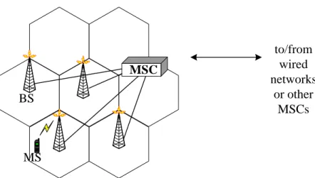
(13) Chapter 2 Related Work. In this chapter, we will introduce the architecture of wireless cellular system, and the basic idea of MINOBJ. Then, the Markov Decision Process with rewards, the policy-iteration method [5] and the state aggregation [6] will be discussed. In MDP, we will give formal definition to state, transition probability, expected immediate rewards, alternatives, policy and gain. Finally, we review some channel allocation strategy, such as guard channel (GC) strategy [4] and borrowing with directional channel-locking (BDCL) strategy [21].. 2.1 Wireless Cellular Networks Wireless mobile networks consist of a fixed network and a large number of mobile terminals including telephone, portable computers, and other devices that can exchange information with remote terminals. In order to effectively utilize the very limited wireless bandwidth to support increasing users day by day, current wireless mobile networks are designed based on a cellular network. The network coverage area is divided into a large number of smaller areas call cells. Each cell has a base station (BS) inside the cell. This BS serves as the network access point for all the terminals in the cell. When a terminal enters into another cell, if the new base station has enough bandwidth to accept, the terminal switches to this new base station. A number of adjacent cells grouped together form an area and the corresponding BSs communicate through a mobile switch center (MSC). The MSC may be connected to other MSCs on the same networks or to other wired networks. A 4.

(14) typical architecture of a cellular network is shown in Fig. 2.1. MSC BS. to/from wired networks or other MSCs. MS. Fig 2.1 A typical architecture of a cellular network. 2.2 Minimizing a Linear Objective Function (MINOBJ) Consider a linear object function, which π denotes the acceptance or rejection of new calls or handoff calls and constant A1 and A2 are penalties of rejecting new call and handoff call respectively. Because we want to give higher priority over handoff call than new call, we only interest in values of A1 and A2 such that 0  A1  A2 .  1n (  2n ) can be 0 or 1 depending on whether the nth new call (the nth. handoff call) is accepted or rejected. Then, we can define the objective function as below N 1 1  N 1    lim E   A11n   A2 2 n  N  N n 0  n 0 . (2.1). We are interested in determining the optimal policy  * over the set of all call admission control policies, i.e., find a policy  * such that  *  min  . We take Eq. . (2.1) as a formulation for the average cost problem [9].. 5.

(15) 2.3 Markov Decision Process The systems we concern about usually contain both probabilistic and decision-making features, so it is too complex to analysis. The Markov Decision Process provides an analytic model for this kind of systems that is easy to describe and computationally feasible.. 2.3.1 State & Transition The basic concepts of Markov Decision Process are those of “state” of a system and state “transition”. A system occupies a state when it can be exactly described by the values of variable that define the state. A system makes state transition when its variable change values specified for one state to those specified for another.. 2.3.2 Transition Probability Suppose that there are N states in the System numbered from 1 to N, then the probability of a transition from state i to state j during a time interval, is a function only about state i and state j and not of any history of the system before its arrival in i. We can specify a set of conditional probabilities pij that a system which now occupies state i will occupy state j after its next transition.. 2.3.3 Rewards Suppose that an N-state Markov Process earns rij dollars when a transition occurs from state i to state j. Then, we call rij the “reward” associated with a transition from state i to state j. We can define vi (n) as the expected total earnings in the next n transitions if the system is now in state i. In order to find vi (n) , we can write the recurrence relation as below. 6.

(16) N. vi (n)   pij [rij  v j (n  1)]. i  1, 2,..., N. n  1, 2,3.... (2.2). j 1. Note that Eq. (2.2) can be written in the form N. N. j 1. j 1. vi (n)   pij rij   pij v j (n  1). i  1, 2,..., N. n  1, 2,3.... (2.3). If a quantity is defined by N. qi   pij rij. i  1, 2,..., N. j 1. Eq. (2.2) takes the form N. vi (n)  qi   pij v j (n  1). i  1, 2,..., N. n  1, 2,3.... (2.4). j 1. 2.3.4 Expected Immediate Reward The quantity qi will be called the “expected immediate reward” for state i which can be interpreted as the reward to be expect in the next transition out of state i.. 2.3.5 Alternatives Fig. 2.2 shows the concept of “alternative”. In the diagram, two alternatives have been allowed, if we choose alternative 1(k=1), then the state transition from state 1 to state 1 will be governed by the probability p111 , the transition from state 1 to state 2 will be governed by p121, and so on. The rewards associated with these transitions are r111, r121, and so on. If the second alternative is chosen (k=2), then p112, p122,…, p1N2 and r112, r122,…, r1N2 would be the transition probabilities and rewards, respectively. In Fig. 2.2, we see if alternative 1 is selected, we make transitions according to the solid. 7.

(17) lines; if alternative 2 is selected, transitions made according to the dashed lines. The number of alternatives in any state must be finite, but the number of alternatives in each state may be different from the numbers in other states.. Present state of system. i=1. Succeeding state of system. p111, r111. j=1. p112, r112 p 2 12 , r. p1 1 2 ,r 12 1. 12 2. i=2. p. 13 2. ,r. 13 2. j=2. p. 13 1. ,r. 13 1. i=3. j=3. i=N. j=N. Fig 2.2 Diagram of states and alternatives. 2.3.6 Policy Let di (n) be the number of the alternatives in the ith state at stage n. When di (n) has been specified for all state i at all stage n, a policy has been determined.. The optimal policy is the one that maximized the total expected earning (or minimizes the total expected earning) for each i and n.. 2.3.7 Gain Consider a completely ergodic N-state Markov process, suppose the process is 8.

(18) allowed to make transitions for a very long time. Then, the total expected earnings depend upon the total number of transitions which system undergoes. A more useful quantity is the average earnings per unit time, called “gain” of the process. We define a state probability  i ( n) , the probability which the system will occupy state i after n transitions if its state at n=0 is known. Since the system is completely ergodic, the limiting state probabilities  i are independent of the starting state, and the gain g of the system is N. g    i qi. (2.5). i 1. 2.4 The Policy-Iteration Method An optimal policy is defined as a policy that maximizes (or minimizes) the total cost. The policy-iteration method that will be described finds the optimal policy in a small number of iterations. It is composed two parts, the value-determination operation and the policy-improvement routine. The iteration cycle is shown in Fig 2.3.. Value-Determination Operation Use pij and qi for a give policy to solve N. g  vi  qi   pij v j. i  1, 2,  , N. j 1. (2.6 ). (2.7) (2.6). for all relative values vi and g by setting v0 to zero. Policy-Improvement Routine For each stat i, find the alternative k’ that maximizes N. qik   pijk v j. (2.8) (2.7). j 1. using the relative values vi of the previous policy. Then k’ becomes the new decision in the ith state, qi k’ becomes qi, and pij k’ becomes pij.. Fig 2.3 The iteration cycle 9.

(19) The upper box, the value-determination operation, yields the g and vi corresponding to a given choice of qi and pij. The lower box yields the pij and qi that increase the gain for a given set of vi. In other words, the value-determination operation yields values as a function of policy, whereas the policy-improvement routine yields the policy as a function of the values. We may enter the iteration cycle in either box. If the value-determination operation is chosen as the entrance point, an initial policy must be selected. If the cycle is to start in the policy-improvement routine, then a starting set of values is necessary. If there is no a priori reason for selecting a particular initial policy or for choosing a certain starting set of values, then it is often convenient to start the process in the policy-improvement routine with all vi = 0. In this case, the policy-improvement routine will select a policy as follows: For each i, it will find the alternative k’ that maximizes qik and then set di = k’. This starting procedure will consequently cause the policy-improvement routine to select as an initial policy the one that maximizes the expected immediate reward in each state. The iteration will then proceed to the value-determination operation with this policy, and the iteration cycle will begin. The selection of an initial policy that maximizes expected immediate reward is quite satisfactory in the majority of cases. At this point it would be wise to say a few words about how to stop the iteration cycle once it has done its job. The rule is quite simple: The optimal policy has been reached (g is maximized) when the policies on two successive iterations are identical. In order to prevent the policy-improvement routine from quibbling over equally good alternatives in a particular state, it is only necessary to require that the old di be left unchanged if the test quantity for that di is as large as that of any other alternative in the new policy determination. In summary, the policy-iteration method just described has the following 10.

(20) properties: 1. The solution of the sequential decision process is reduced to solving sets of linear simultaneous equations and subsequent comparisons. 2. Each succeeding policy found in the iteration cycle has a higher gain than the previous one. 3. The iteration cycle will terminate on the policy that has largest gain attainable within the realm of the problem; it will usually find this policy in a small number of iterations.. 2.5 The State Aggregation Method One of the principal methods for solving the MINOBJ problem is the policy-iteration method which iterates between the policy-improvement routine like Eq. (2.7) that yielding a new policy, and the value-determination operation that finds the total-value vector v(n) corresponding to policy by solving Eq. (2.6). But Eq. (2.7) is a linear n × n system which can be solved by a direct method such as Gaussian elimination. In the absence of specific structure, the solution requires O(n3) operations, and is impractical for large n. An alternative, suggested in [10], [11] and widely regarded as the most computationally efficient approach for large problem, is to use an iterative technique for the solution for Eq. (2.6), such as the successive approximation method in [12]; this requires only O(n2) per iteration for dense matrix P. It appears that the most effective way to operate this type of method is not to insist on a very accurate iterative solution of Eq. (2.6). The idea here is to solve this system with smaller dimension, which is obtained by lumping together the states of the original system into subsets S1, S2, …, Sm that can be viewed as aggregate states. These subsets are disjoint and cover the entire state space S. 11.

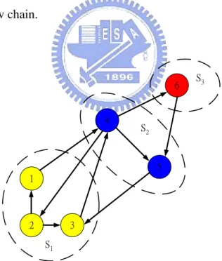
(21) Consider the n × m matrix W whose ith column has unit entries at coordinates corresponding to states in Si and all other entries equal to zero. Consider also an m × n matrix Q such that the ith row of Q is a probability distribution with qis = 0 if s not belongs to Si. The structure of Q implies two useful properties: 1. QW = I. 2. The matrix T = QPW is an m × m transition probability matrix. In particular, the ijth component of T is equal to tij and gives the probability that the next state will belong to aggregate state Sj given that the current state is drawn from the aggregate state Si according to the probability distribution qis. The transition probability matrix T defines a Markov chain, called the aggregate Markov chain, whose states are the m aggregate states. Fig. 2.4 illustrates an example of aggregate Markov chain.. 6. 4. S3. S2. 5 1. 2. 3 S1. Fig. 2.4 An example of the aggregated Markov chain. In this example, the aggregate states are S1  1, 2, 3 , S 2  4, 5 , and S3  6 . The matrix W has columns (1, 1, 1, 0, 0, 0)', (0, 0, 0, 1, 1, 0)', and (0, 0, 0, 0, 0, 1)'. The matrix Q is chosen so that each of its rows defines a uniform probability. 12.

(22) distribution over the states of the corresponding aggregate state. Thus the rows of Q are (1/3, 1/3, 1/3, 0, 0, 0), (0, 0, 0, 1/2, 1/2, 0), and (0, 0, 0, 0, 0, 1). The aggregate Markov chain has transition probabilities t11 = t21 =. 1 2.  p42 + p53  , t22 =. 1 2. p 45 , t23 =. 1 2. 1 3. 1.  p21 + p23  , t12 =  p14 + p34  , t13 = 0, 3. p46 , t31 = 0, t32 = p56 , and t33 = 0.. Aggregate Markov chains are most useful when their transition behavior captures the broad attributes of the behavior of the original chain. This is generally true if the states of each aggregation state are “similar” in some sense.. 2.6 Guard Channel Strategy The concept of guard channels was introduced in the mid-80s, as a call admission control to give priority to handoff calls over new calls [7]. In this strategy, a fixed portion of channels called guard channels is permanently reserved for handoff calls, and the remaining channels can be used for both handoff calls and new calls. In [8], Miller obtains a result, which can be used to show that the Guard Channel policy is optimal for the MINOBJ problem. Denote C as the number of channels in each cell. The Guard Channel Strategy will reserve a subset of channels (C-T) for handoff calls. When the number of channel assigned to calls exceeds a certain threshold T, the guard channel strategy only accept handoff call and rejects new calls until the channel occupancy goes below the threshold. Note that this strategy accepts handoff calls only if the cell has available channel. This algorithm is illustrated with Fig. 2.5.. 13.

(23) Call Arrival. Handoff Call. Current State <C. YES. YES. Is Handoff Call ?. Accept Call. NO. YES. New Call. Current State <T. NO. NO. Drop Call. Reject Call. Fig 2.5 Guard Channel Strategy. 2.7 Borrowing with Directional Channel Locking (BDCL) In the fixed assignment (FA) assignment, a set of nominal channels is assigned to each cell. If all nominal channels are assigned, new calls are blocked. Under this scheme, some cells may have large blocking rate but some may have a lot of unassigned channels. This will waste the bandwidth and decrease the quality of service (QoS). Therefore, the dynamic channel assignment strategies are proposed, and BDCL is one of them. Elnoubi and Singh [21] proposed a strategy, “borrowing with channel-ordering” (BCO). In the BCO strategy, if a channel is borrowed, it is locked in the co-channel cells within the channel reuse distance of borrowing cell. Being locked means that the channel can’t either be used or be borrowed to the neighboring cell. This kind of borrowing therefore carries a penalty. Zhang and Yum proposed a new strategy, borrowing with directional. 14.

(24) channel-locking (BDCL) [21]. When a channel is borrowed, the locking of this channel in the co-channel cells is restricted only to those affected by this borrowing. Therefore, the number of channel available for borrowing is greater than those of BCO strategy.. 2. 1 0. 3 2. 1 0. 3. 4. 4 6. 5 2. 1 0. 3. 4. x. 0. 4. 4. 1 0. 3. 4. 5 1 0. 3. 5. 6. 2. 6. 2. 6. 5. 1. 1 0. 3. 5 2. 3. 2. 6. 4. 6. 5. 6. 5. Fig 2.6 An example of BDCL. In BDCL strategy, a set of nominal channels is assigned to each cell, and the co-channel cells use the same set of nominal channels. The major difference between BDCL strategy and FA strategy is that the base cell can borrow channels from the adjacent cells in the BDCL strategy. In order to minimize the blocking of later calls, the general rule is to borrow channel from the richest adjacent cell. The richest cell means it has the most unused channels. We will introduce it in the following example and illustrated as the above Fig 2.6:. 15.

(25) When a call arrives, Cell 0 (base cell) doesn’t have any available channel. It attempts to borrow a channel from the neighboring cells. Before borrowing a channel, Cell 0 has to check which adjacent cell is the richest cell that owns the most number of nominal channels not used and not locked. If the richest adjacent cell of Cell 0 is Cell 3, it has to borrow the channel that is not used from Cell 3. After making the decision of the borrowing channel, the co-channel cells of Cell 3 in the interference region of Cell 0, Cell 3 and Cell 3’s as Fig 2.6, have to be locked and to lock the channel in the proper directions to the neighboring cells of them. The locking of the channel means the cell that owns the channel as the nominal channel can not use it and the cell that does not own the channel can not borrow it. One more characteristic is that the set of the nominal channels for each cell have different priorities, from the highest to the lowest. Each cell uses the self channel with the highest priority of them and borrows the channel with the lowest priority of them from the richest neighboring cell.. 16.

(26) Chapter 3 Problem Formulation by MDP and Proposed Method. In this chapter, we introduce how to formulate our system into a two-dimensional Markov Decision Process and how to find the optimal policy. The optimal policy means which action should be taken with the least cost for BS. We then use the policy-iteration method and state aggregation method to solve the problem of MINOBJ. In the case of single-service networks, Krishnan and Ott [15], and Lazarev and Starobinets [16] have proposed state dependent routing schemes with roots in Markov decision theory. We use the separable routing concept defined by Krishnan and Ott which is appropriately modified for the case of cellular networks. We also study the problem of call admission control where we follow Zachary’s procedure [17] to determine the cost of rejecting new calls and dropping handoff calls.. 3.1 System Specification We consider our mobile communication network as a cellular network. In our cellular structure, each cell is surrounded by six cells. A mobile staying in a cell can communicate with another terminal, which may be a node of the wired network or other mobile, through the base station in the cell. When it moves to an adjacent cell, a handoff will enable the mobile to maintain connectivity, i.e., the mobile will connect through another base station without noticing any difference. We preclude 1) delay-insensitive application, which might tolerate long handoff delays in case of insufficient bandwidth available in the new cell at the handoff time 17.

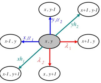
(27) and 2) soft handoff of the Code Division Multiple Access (CDMA) systems [13],[14], in which a mobile can communicate via two adjacent base stations simultaneously for a while before actual handoff takes place.. 3.2 MDP-based Cellular System Model 3.2.1 Model Assumptions In our model, we assume that each cell is allocated with a fixed set of channels and each connection uses equal bandwidth (one channel). A two-dimensional Markov Chain is used to model the system. The first dimension is made of base cell’s channel state and represents how many channels are used presently. The second dimension is made of all adjacent cells and represents how many channels are used by all adjacent cells. New call arrival in the base cell and adjacent cells are according to a stationary Poisson process with mean rate λ1 and λ2, respectively. The call holding time in the base cell and adjacent cells are independent and exponential distributed with mean μ1 and μ2, respectively. Call handoff from the base cell to adjacent cells and from adjacent cells to base cell are also exponential distributed with rate h1 and h2, respectively. We consider a homogeneous system where each cell can support up to C calls, the cell state vector n(t) which provides the complete state description of the cell at any time instant is defined as. n(t )  ( x, y), n  N. (3.1). Where x is the number of calls in the base cell at time t, and y is the number of calls in all adjacent cells at time t. The cell state space is denoted by N, which contains a finite but large number of states. The state transition diagram is shown in Fig 3.1.. 18.

(28) x , y-1. yμ2 xμ1. x-1 , y. xh1 x-1 , y+1. x,y. x+1 , y-1. yh2. λ1. x+1 , y. λ2 x , y+1. Fig 3.1 State transition diagram. The parameters which accompany transition lines divide by τ are transition probabilities. τ is given as.   1  2  x( 1  h1 )  y ( 2  h2 ). (3.2). 3.2.2 Alternatives and Costs The MDP with costs has been the means to an end. It is the analysis of decisions in sequential process that are Markovian in nature [5]. We will introduce alternatives and costs of sequential decision process and define them in this section. In our model, we have two alternatives when a new call or a handoff call comes: Alternative 1: accept Alternative 2: reject. We define that a cost ω1 is incurred when a new call is reject by base station and a cost ω2 is incurred when a handoff call is reject by base station. By these definitions, there are different behaviors with corresponding alternatives. So, we can make a different state transition diagram in Fig 3.2 that base station admits a new (or handoff) call incur nothing but rejects it with cost ω1 (or ω2). These analyses will help us to 19.

(29) find the solution of the sequential decision process.. x , y-1. x+1 , y-1. yh2,ω2. yμ2. yh2 x-1 , y. xμ1 xh1. x-1 , y+1. x,y. Alternative 1: Accept. λ1. x+1 , y. Alternative 2: Reject. λ 1, ω 1. λ2 x , y+1. Fig 3.2 State transition diagram with alternatives. All alternatives that could be taken by base cell’s state are listed in Table 3.1 below.. Table 3.1 alternatives of base cell’s state Alternatives. New Call. Handoff Call. 0. block. drop. 1. accept. drop. 2. block. accept. 3. accept. accept. 3.3 Our Policy-Iteration Method An optimal policy is defined as a policy that minimizes the cost. It is conceivable that we find the cost for each of these alternatives in order to find the policy with the least cost. We are interested in finite horizon systems and we know the appropriate objective is the average cost optimization. It means that our goal is to minimize the 20.

(30) expected rate of cost due to lost calls. We can denote Vπ (t) the lost revenue in the cell during the time interval [0,t] under the policy    , where  is the set of all policies. Then, using the result from [5], we have the expected value. E[V (t | n0  n)]  g t  v (n)  o(1), (t  ). (3.3). where n  N is the cell state at time t=0. In Markov decision theory, vπ (n) is the well-known relative value or cost of starting in state n0=n. In Eq. (3.3), gπ represents the expected cost per unit time under the policy π on the original continuous-time scale. Since the system is ergodic, we may call gπ as the gain of the process. The objective is to minimize the equilibrium expected cost per unit time, gπ . The “small o” symbol o(1) means that for both the right hand side (RHS) and the left hand side (LHS) of the equation go to infinity, and the difference goes to zero. Before to find the relative cost values vπ (n) , we define two vectors 1 0  ek 2 , ek    0 1   1 1  f k 2 , f k     1 1. (3.4) (3.5). Then, in the case of the departure of a call when the cell state is n, the immediately subsequent state d k (n)  N is found as d k (n)  n  ek. (3.6). A new call admission decision needs to be made at call attempt epochs: either accept or block. Denoting an alternative taken on the arrival of a call by πk(n) where n  N is the current cell state. In the case of call rejection. 21.

(31)  k ( n)  n. (3.7). If the new call is accept, the subsequence state of the cell will be found as.  k (n)  n  ek. (3.8). A handoff cal admission decision needs to be made at call across the cell boundary epochs: either accept or drop. Use the same definition above, in the case of dropping a handoff call.  k (n)  n  ek. (3.9). If the handoff call is accepted, the subsequent state of the cell will be found as.  k ( n)  n  f k. (3.10). Now we start to introduce how to find the relative cost values vπ (n) for all n  N . The same equation also governs the asymptotic behavior of the process if we. assume that it has started immediately after the first event that has occurred after t=0. This is because of the ergodic nature of the system, where the initial state has no effect on the asymptotic behavior of the process far enough in the nature. The first event is either a cell termination or a new (handoff) call arrival. The expected time τ for the first event after t=0 is given as. . 1. . 2. ,    [k  nk (hk  k )]. (3.11). k 1. where we used the memoryless property of the system. Writing Eq. (3.3) for a starting time t=0 and a first event time t=τ(the latter one is conditional on the type of the first event), we obtain after some arrangements 2. 2. v (n)  g    nk k v (d k (n))   k [ k (n,  k (n))1  v ( k (n))] k 1. k 1. 2.    nk hk [ k (n  ek ,  k (n))2  v ( k (n))] , n  N k 1. 22. (3.12).

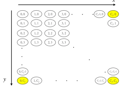
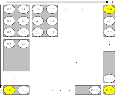
(32) where  k () is the Kronecker symbol as follows. 1, if n   k (n) 0, otherwise..  k (n,  k (n))  . (3.13). In the system of linear Eq. (3.12), the unknown variables are vπ (n) for all n  N , and the gain of the process gπ . Obviously, the system has one more variable than the number of equations so that v () s can be determined up to an additive constant. To solve the system Eq. (3.12), we follow the standard procedure by setting vπ (0)=0. Thus, we get the system 2. g   k [ k (0,  k (0))1  v ( k (0))] k 1. 2.   nk hk [ k (0,  k (0))2  v ( k (0))]. (3.14). k 1. 3.4 Our State Aggregation Method In Fig 3.3, the first dimension is made of base cell’s channel state, where C1 is the fixed link capacity C. The second dimension is made of all adjacent cells’ channel state, where C2 is six times of the fixed link capacity C. The total states of this two-dimensional Markov chain are C1  C2 .. 23.

(33) x 0, 0. 1, 0. 2, 0. 3, 0. 0, 1. 1, 1. 2, 1. 3, 1. C1: total capacity of Base Cell. 0, 2. 1, 2. 2, 2. 3, 2. 0, 3. 1, 3. 2, 3. 3, 3. C2: total capacity of Adjacent Cells. ‧. ‧. ‧. ‧. C1, 0. C1-1, 0. C1, 1. ‧. ‧. ‧. ‧ 0, C2-1. y. 0, C2. ‧ 1, C2. ‧. ‧. ‧. C1-1, C2. C1, C2-1. C1, C2. Fig 3.3 Total state diagram of the two-dimensional Markov chain. When using Guassian elimination method to solve Eq. (3.12), we will face the same problem already described in section 2.6. The inverse matrix of transition probability matrix P is of complexity O(n3), which is impractical for large n. We can take the Guard Channel policy mentioned in section 2.2 for an example. The threshold T will divide the states of the cell into three groups. From state 0 to T is first group which can accept all kinds of calls. From state (T+1) to (C-1) is second group which can accept only handoff calls. The third group is state C. When in third group, no call can be accept due to unavailable of all the channels. Thus, we can learn from this example grouping states which are few steps reachable in the neighborhood. We use the method like quantization to divide the first dimension of Markov chain into even size, excluding the last state is an independent group. The second dimension is divided with the same way. The two-dimensional Markov chain can be grouped as shown in Fig 3.4 below.. 24.

(34) x 0, 0. 1, 0. 2, 0. 3, 0. 0, 1. 1, 1. 2, 1. 3, 1. C1, 1. 0, 2. 1, 2. 2, 2. 3, 2. C1, 2. 0, 3. 1, 3. ‧. ‧. C1, 0. ‧. ‧ ‧ ‧ ‧. ‧. ‧. ‧ ‧ ‧. y. 0, C2. C1, C2-1. 1, C2. ‧. ‧. ‧. C1-1, C2. C1 , C2. Fig 3.4 Make two-dimensional Markov chain into smaller groups. 3.5 Parameters Estimation This section addresses parameters estimation of our strategy. In our model, we use call arrival rate, handoff rate and departure rate in MDP to find the optimal policy. Nevertheless, these parameters will vary with time. In order to make our model closer to the actual, we adjust these parameters and update policy periodically. Since these parameters vary from time to time, how to estimate efficiently is now we concerned about.. 3.5.1 Cost Match Update Rule We use cost match update (CMU) rule to help us to estimate. This method just can estimate a parameter. It adjusts the parameter by using the difference between system cost and model cost. The system cost is induced by reality and the model cost is defined by our model. If system cost is different from model cost, it means our model did not match the reality, and we should change parameter to make model more close to the reality. For example, if we use CMU rule to adjust adjacent cells’ new call arrival rate. 25.

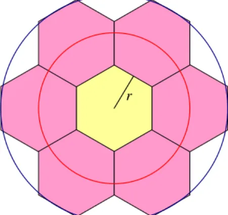
(35) Then, if the system cost is larger than model cost, it means adjacent arrival rate may be underestimated and we should increase adjacent arrival rate. Actually, we use CMU rule to adjust adjacent cells’ arrival rate, because how precise the estimation of adjacent arrival rate is not only effect adjacent arrival rate, but also effect handoff-in rate. So, we choose it to use CMU rule and other parameters use sample mean to estimate. In our simulation, it indeed does work. The model cost is defined as Eq. (3.14), and the system cost is the sum of blocking new calls’ costs and dropping handoff calls’ costs in every time unit.. 3.5.2 State Adjustment For base cell, the factor effects the handoff rate is not only the number of mobiles in the adjacent cells, but also the positions of mobiles in the adjacent cells. In our model, we give mobile different weight according to the mobiles’ real-time position when we calculate cell state. We can use Eq. (3.15) to show the state the number of adjacent cells’ mobiles after adjustment.. # of adjacent cells ' mobiles   i. 3r  distance(mobilei , BS ) r. (3.15). Briefly, if the distance between the mobile and base station in base cell is r, the weight of the mobile is 2. If the distance between the mobile and base station in base cell is 2r, the weight of the mobile is 1. If the distance between the mobile and base station in base cell is 3r or more, the weight of the mobile is 0. Others are also stand on this way depending on distance giving different weight.. 26.

(36) r. 3r  distance(mobile, BS ).  position to Fig 3.5 Illustration of using mobile’s r calculate cell state # of Adjacent cells ' mobiles . 3.6 MDP-based Call Admission Control in BDCL In this section, we will introduce how we modified the previous MDP model of FCA strategy to BDCL strategy. In order to get optimal policy, we use one-step policy which will use the previous computational result of FCA. The main difference between FCA strategy and BDCL strategy is “borrowing” action. We modify our state transition diagram with alternatives to fit BDCL strategy. In BDCL, we have three alternatives when a new call (or handoff call) comes: Alternative 1: accept Alternative 2: reject Alternative 3: borrow. 27.

(37) x , y-1. yh2,ω2 yh2,ω3. yμ2. x-1 , y. x+1 , y-1. xμ1. λ1. x,y. xh1. x+1 , y. λ 1, ω 1 λ 1, ω 3. λ2. x-1 , y+1. Alternative 1: Accept. yh2. Alternative 2: Reject Alternative 3: Borrow. x , y+1. Fig 3.6 State transition diagram with alternatives for BDCL. The cost ω3 is incurred with alternative 3 when a call (either new cell or handoff call) arrives, base station borrows channel from adjacent cell. The cost ω3 is not fixed, and it will vary with all the cells in interference region effecting by borrowing action including which channel are borrowed and the state of all these cell after borrowing. There will be an example illustrated in Fig 3.7 below. For co-channel cells (3). 0. 3. Pr 1. 4. If ch-x is locked. 0. 3. 5. Pr. x, y 6. 0. 3. 4. 5. 2. 3. x. 1 0. 4. x+1, y. If ch-x is not locked 2. 6. For other cells 2. 3. 1 0. 4. 5 2. 6. 3. 3. 0. 1 0. Fig 3.7 An example of borrowing operation. 28. Pr. x, y Pr. If ch-x is locked If ch-x is not locked. x, y+1.

(38) In the red line bounded region, if cell 0 borrows channel-x from cell 3, the state transitions of the cells in this region is illustrated in Fig 3.8. State transitions in these cells can be separate into two groups, co-channel cells and non-co-channel cells.. For co-channel cells (cell 3). For other cells. Pr. x, y. Pr. Pr. x, y. If ch-x is locked x+1, y. Pr. If ch-x is not locked. If ch-x is locked If ch-x is not locked. x, y+1. Fig 3.8 transition diagram of all the cells in interference region Then, the borrowing costω3 can be derived as below N. 3   V jk (n  1) - Vi k (n) . (3.16). k 1. N : number of cells in the interference region Vi k (n) : Value of current state i current stage n for adjacent Cell k V jk (n  1) : Value of next state j next stage n  1 for adjacent Cell k i  j , the selected channel to borrow is locked  i  j , the selected channel to borrow is not locked When a call (either new call of handoff call) arrives, we have to check all unused channels of adjacent cells and get the channel which causes the least cost ω3. The channel that causes the least cost of ω3 is selected to be borrowed if alternative 3 is the best alternative to borrow. All alternatives for BDCL that could be taken by base cell’s state are listed in Table 3.1 below.. 29.

(39) Table 3.2 alternatives of base cell’s state for BDCL. Alternatives. New Call. Handoff Call. 0. block. drop. 1. accept. drop. 2. borrow. drop. 3. block. accept. 4. accept. accept. 5. Borrow. accept. 6. block. borrow. 7. Accept. borrow. 8. borrow. borrow. There are 9 alternatives for base station listed above, we use the state value of previous result and derive the policy to fit our model. This policy is not the optimal policy but is the improved one. We use one-step policy, which is only taken Policy Improvement Routine in Policy-Iteration method introduced in section 2.5. It is proved that one-step policy although is not the optimal policy, but it is closed to the optimal one [5].. 30.

(40) Chapter 4 Simulation Results and Performance Analysis. 4.1 Simulator Settings The simulated cellular system contains 98 hexagonal cells (i.e. a 14  7 mesh) as shown in Fig 4.1 with white background. This is a simple case can be extended to implement in large area. The boundary cells will have fewer mobiles because there are no mobiles entering from outside of cellular system, and then cells near the center will be more crowed by mobiles than those near the borders. Therefore, we connected all boundary cells of cellular structure as the gray background cells in Fig 4.1.. 97 6. 1. 0. 20. 15. 14 27. 21 28. 34. 29. 42. 56. 76 83. 77 85. 97. 86 92. 91 0. 79. 1. 80. 93 2. 94 3. 95 4. 63 70. 76 83 90. 77 84. 97. 96 5. 56 69. 82 89. 49. 55. 68. 81. 35 42. 62. 75. 88. 41 48. 61. 21 28. 34. 54. 67 74. 87. 14 27. 40. 53. 7. 13 20. 47. 60. 73. 72. 39 46. 66. 0. 26 33. 52. 65. 78. 19. 39. 97 6. 12. 25 32. 59. 58. 11 18. 45 51. 64 71. 84. 37. 50. 5. 24 31. 44. 57. 70. 90. 36. 63. 69. 17 23. 30. 43 49. 55 62. 16. 96. 95 4. 10. 9. 22. 35. 41 48. 94 3. 2 8. 7. 13. 93. 92. 91. 6. 91 0. Fig 4.1 Cellular structure of simulation. All cells are assigned with 50 channels, and each connection use 1 channel. The channel reuse distance is assumed to be three cell units. We assume new call are 31.

(41) generated according to a Poisson process with rate λ=500 – 1500 calls/per hour, but each cell is under different traffic load. The lifetime of each call is exponential distributed with the mean 3 min. We incorporate road layouts that place constraints on mobiles’ paths, thus establishing a more realistic platform to evaluate the performance. The radius of each cell is 2 km and mobile velocity is from 30km/hr to 90km/hr with 5% variance. Fig 4.2 is part of load layout in our simulation.. Fig 4.2 Part of road layout in our simulation. There are total 51 301 states, and it will take too much time to compute, so we use the aggregation method mentioned in section 3.4 to aggregate states into groups. In our model, we aggregate to total 6 11 states as shown in Table 4.1 below. This is a compromise between computing complexity and the difference of the result derived. Note that the last column (with gray background) of Table 4.1 is mode of only one previous state, because no matter a new call or handoff call arrives in that state, it will not be accepted due to unavailable of all the channels in the base cell.. 32.

(42) Table 4.1 Aggregation of total states. Adjacent Cells’ Group. Base Cell’s Group Cell’s States 0~9 10~19 20~29 30~39 40~49 50 (after aggregation) 1 2 3 4 5 6 0~29 1 0 1 2 3 4 5 30~59 2 6 7 8 9 10 11 60~89 3 12 13 14 15 16 17 90~119 4 18 19 20 21 22 23 120~149 5 24 25 26 27 28 29 159~179 6 30 31 32 33 34 35 180~209 7 36 37 38 39 40 41 210~239 8 42 43 44 45 46 47 240~269 9 48 49 50 51 52 53 270~299 10 54 55 56 57 58 59 300 11 60 61 62 63 64 65. 4.2 Simulation Results In the guard channel strategy, threshold T represents number of channels reserved for handoff calls. If T is large, the handoff force terminating rate will decrease but the new call blocking rate will increase. We use Guard Channel strategy with different threshold T to decide how many channels reserved for handoff calls is better. The result is shown in Fig 4.3 below.. In Fig 4.3, we can see that when threshold T is 45, the dropping rate is almost equal to T=44 and is not too high, but the blocking rate is lower then T=44. So, we choose T=45 as the threshold of our Guard Channel Strategy.. 33.

(43) Fig 4.3 Guard Channel Strategy with different threshold. The performance of MDP-based call admission control with CMU rule is compared with the fixed channel allocation (FCA), Guard Channel strategy with threshold 45 (GC), and MDP-based call admission control without CMU rule. It is shown in Fig 4.4 to Fig 4.6.. Fig 4.4 Dropping rate versus traffic load in FCA 34.

(44) Fig 4.5 Blocking rate versus traffic load in FCA. Fig 4.6 Ave. Cost (per mobile) versus traffic load in FCA. 35.

(45) Fig 4.4 compares dropping rate versus traffic load. Dropping rate is defined as the percentage of handoff calls can not be allocated to a channel in all served calls. Fig 4.4 shows that dropping rate of FCA is highest, because FCA does reserve any channel for handoff call. Dropping rate of MDP-based call admission control with CMU rule is lower than GC. Fig 4.5 compares blocking rate versus traffic load. Blocking rate is defined as the percentage of new call which can not be allocated to a channel in all arriving calls. Fig 4.5 shows that blocking rate of FCA is lowest. Blocking rate of MDP-based call admission control with CMU rule is higher than GC. In Fig 4.6, we can see our proposed method has the lowest average cost. Besides, our proposed method performs better than MDP-based call admission control without CMU rule. It shows CMU rule is effective. In Fig 4.7 to Fig 4.9, we will show the performance of MDP-based call admission control with CMU rule in BDCL compares to BDCL and the GC with BDCL. The strategy of GC with BDCL is if new call arrives and the number of using channel is equal or larger than threshold, we block this call. If handoff call arrives and all the channels in base cell are unavailable, we still do not drop this call unless there is no available channel in adjacent cells. Fig 4.7 compares dropping rate versus traffic load. Fig 4.7 shows that dropping rate of BDCL is highest, because BDC does reserve any channel for handoff call. Dropping rate of MDP-based call admission control with CMU rule is similar to GC with BDCL. Fig 4.8 compares blocking rate versus traffic load. Fig 4.8 shows that blocking rate of BDCL is lowest. Blocking rate of MDP-based call admission control with CMU rule is lower than GC with BDCL under load less than 110, but higher than GC with BDCL when the traffic load is larger than 110. In Fig 4.9, we can see our 36.

(46) proposed method has similar average cost to GC with BDCL.. Fig 4.7 Dropping rate versus traffic load in BDCL. Fig 4.8 Blocking rate versus traffic load in BDCL. 37.

(47) Fig 4.9 Ave. Cost per mobile versus traffic load in BDCL. 38.

(48) Chapter 5 Conclusion. In our thesis, we formulate the call admission control problem into a minimizing linear cost function of blocking rate and dropping rate. In our model, the adjacent cells’ mobile information is taken into consideration including number of mobiles, new calls arrival rate, handoff rate, departure rate and mobile position information. We formulate our model based on MDP and use Policy-Iteration method to solve. In order to reduce the computation complexity, we use state aggregation method to decrease the number of states. We use several parameters like arrival rate, handoff rate, departure rate, to formulate our model, but these parameters vary with time. How to estimate these parameters precisely to make our model more close to the reality is what we care about. We use Cost Match Update (CMU) rule to adjust adjacent cells’ new call arrival rate and use sample mean to adjust other parameters, then the base station can update policy periodically. In our simulation results, we can see that the average costs of our proposed method are lower than Guard Channel strategy. It reveals our estimation method can indeed help our model to perform better.. 39.

(49) References [1] S. Tekinay and B. Jabbari, “Handover and Channel Assignment in Mobile Cellular Networks,” IEEE Commun. Mag., vol. 29, no. 11, Nov. 1991. [2] E. C. Posner and R. Guerin, “Traffic Policies in Cellular Radio that Minimizing Blocking of Handoff Calls,” in Proc. 11th Teletraffic Cong. (ITC 11), Kyoto, Japan, Sept. 1985. [3]. S. Choi and K. G. Shin, “Adaptive Bandwidth Reservation and Admission Control in QoS-Sensitive Cellular Networks,” IEEE Trans. Parallel and Distributed Sys., vol. 13, no. 9, pp. 882–897, Sep. 2002.. [4]. R. Ramjee, D. Towsley, and R. Nagarajan, “On Optimal Call Admission Control in Cellular Networks,” Wireless Networks Journal, vol. 3, no. 1, pp. 29-41, March 1997.. [5] R. A. Howard, Dynamic Programming and Markov Processes, MIT Press, 1960. [6] D. P. Bertsekas, Dynamic Programming and Optimal Control, vol. 2, 2nd edition, Athena Scientific, Belmont, Massachusetts, 2000. [7]. D. Hong and S. S. Rappaport, “Traffic Model and Performance Analysis for Cellular Mobile Radio Telephone Systems with Prioritized and Nonprioritized Handoff Procedures,” IEEE Trans. on Vehicular Tech., vol. 35, no. 3, pp. 77-92, Aug. 1986.. [8] B. L. Miller, “A Queuing Reward System with Several Customer Classes,” Management Science, vol. 16, no. 3, pp. 234-245, 1969. [9] D. P. Bertsekas, Dynamic Programming: Deterministic and Stochastic Models, Prentice-Hall, Englewood Cliffs, NJ, 1987. [10] M. L. Puterman and M. C. Shin, “Modified Policy Iteration Algorithms for Discounted Markov Decision Problems,” Management Science, vol. 24, no. 11, pp. 1127-1137, Jul. 1978. [11] M. L. Puterman and M. C. Shin, “Action Elimination Procedures for Modified Policy Iteration Algorithms,” Operations Research, vol. 30, no. 2, pp. 301-318, 1982. [12] E. L. Porteus, “Overview of Iterative Methods for Discounted Finite Markov and Semi-Markov Decision Chains,” in Recent Developments in Markov Decision Process, R. Hartley et. al. (eds.), New York: Academic Press, 1980. [13] D. Collins and C. Smith, 3G Wireless Networks, McGraw-Hill, 2001. [14] A. J. Viterbi, CDMA: Principles of Spread Spectrum Communication, Reading, 40.

(50) Mass.:. Addison-Wesley, 1995.. [15] T. J. Ott and K. R. Krishnan, “State Dependent Routing of Telephone Traffic and the Use of Separable Routing Schemes,” in Proc. 11th Teletraffic Cong. (ITC 11), Kyoto, Japan, Sept. 1985. [16] V. G. Lazarev and S. M. Starobinets, “The Use of Dynamic Programming for Optimization of Control in Networks of Communications of Channels,” Eng. Cyber., vol. 15, pp. 107-116, 1977. [17] S. Zachary, “Control of Stochastic Loss Networks, with Applications,” J. Roy. Statist. Soc. Ser. B, vol. 50, pp. 61-73, 1988. [18] A. Jayasuriya, D. Green and J. Asenstorfer, “Modeling Service Time Distribution in Cellular Networks Using Phase-Type Service Distributions, ” in Proc. IEEE Int. Conf. on Communications (ICC 2001), vol. 2, pp. 440-444, Helsinki, Finland, June 2001. [19] F. Barcelo and J. Jordan, “Channel Holding Time Distribution in Cellular Telephony,” The 9th International Conference on Wireless Communications (Wireless’97), vol. 1, pp. 125-134, Alberta Canada, 9-11 July, 1997. [20] S. M. Elnoubi, R. Singh, and S. C. Gupta, A new frequency channel assignment algorithm in high capacity mobile communication systems, IEEE Trans. Veh. Technol., vol. VT-31, no. 3, pages 294-301, 1982. [21] M. Zhang and T.-S. Yum. “Comparisons of channel assignment strategies in cellular mobile telephone systems.” IEEE Trans. on Vehicular Technology, Vol. 38, no. 4, pages 211{215, Nov., 1989. [22] Kshirasagar Naik and David S.L. Wei and Stephan Olariu, “Channel Assignment in Cellular Networks with Synchronous Base Stations, ” PEWASUN’ 05, October 10–13, 2005, Montreal, Quebec, Canada. [23] Chia-Fu Chen, “Markov-Decision-Based Call Admission Control with Neighboring State Information in Cellular Networks, ” in NCTU, Dec 2006. [24] Hsien-Tsung Tsao, “Markov-Decision-Based Call Admission Control with State Information of Adjacent Cells in Road-based Cellular Networks, ” in NCTU, May 2008.. 41.

(51)