微型揚聲器振膜刻痕最佳化與低頻延伸設計

全文

(1)國立交通大學機械工程研究所碩士論文微型揚聲器振膜刻痕最佳化與低頻延伸設計. Optimized Design of Diaphragm Patterns and Bass reflex enclosures of Microspeakers. 指導教授：白明憲研究生：劉青育. 中華民國九十七年七月.

(2) 微型揚聲器振膜刻痕最佳化與低頻延伸設計 Optimized Design of Diaphragm Patterns and Bass reflex enclosures of Microspeakers. 研究生：劉青育. Student：Ching-Yu Liou. 指導教授：白明憲. Advisor：Mingsian R.Bai. 國立交通大學機械工程學系碩士論文. A Thesis Submitted to Institute of Mechanical Engineering College of Engineering National Chiao Tung University In Partial Fulfillment of Requirements For the Degree of Master of Science In Mechanical Engineering July 2008 HsinChu, Taiwan, Republic of China.. 中華民國九十七年七月 i.

(3) 微型揚聲器振膜刻痕最佳化與低頻延伸設計研究生：劉青育. 國立交通大學. 指導教授：白明憲. 機械工程研究所. 教授. 碩士班. Abstract 今日用於行動配備的微型揚聲器總是被需求微小化、高輸出等級、高聲音品質等特性，但這些需求都存在著矛盾關係。相對於大型揚聲器，微型揚聲器的結構簡化了懸吊裝置。微型揚聲器振膜的作用不僅可以幅射出聲音亦可以當作懸吊系統。因此振膜上的刻痕設計對於微型揚聲器的性能與頻率響應是很重要的。傳統用集中參數的方法一般是不足以模擬到振膜高頻撓性共振的模態，因此在這篇論文中結合了有限元素分析與機電聲類比電路的方法，比起以往傳統的方法能夠更準確的模擬出微型揚聲器的性能。尤其在計算音圈與振膜機械阻抗時，是利用有限元素分析來求得的，再將所求得的機械阻抗代入機電聲類比電路的機械系統中，接著求解機電聲迴路方程式即可模擬微型揚聲器的性能響應。以此模擬平臺，使用田口分析法對振膜刻痕做最佳化分析，另外再利用敏感度分析求得振膜最佳刻痕數。在此篇論文中也提到結合有限元素分析與集中參數的方法來模擬音箱系統及. i.

(4) 利用約束最佳化方法對音箱尺寸做最佳化分析。另外也提到結合類神經網路與模擬退火法對微型揚聲器振膜做最佳化分析。. ii.

(5) Optimized Design of Diaphragm Patterns and Bass reflex enclosures of Microspeakers. Student: Ching-Yu Liou. Advisor：Mingsian R.Bai. Institute of Mechanical Engineering National Chiao-Tung University. Abstract Today’s microspeakers of portable devices are demanded to meet a number of conflicting requirements including miniaturization, high output level, good sound quality, etc.. In contrast to large loudspeakers, the structures of microspeakers are. generally simplified enough with suspension removed. only a sound radiator but also the suspension.. The diaphragm serves as not. Thus, the pattern design of the. diaphragm is crucial to the overall response and performance of a microspeaker. Traditional approach for modeling microspeakers using lumped-parameter models is generally incapable of modeling flexural modes in high frequencies. In this paper, a hybrid approach that combines finite element analysis (FEA) and electro-mechanoacoustical (EMA) analogous circuit is presented to provide a more accurate model than the conventional approaches. In particular, the minute details of diaphragms are taken into account in calculating the mechanical impedance of the diaphragm-voice coil assembly using the FEA.. The mechanical impedance obtained using FEA is. incorporated into the lumped parameter model. The responses can be simulated by solving the loop equations.. On the basis of this simulation model, the pattern design. of the diaphragm is optimized using the Taguchi method. iii. In addition, the optimal.

(6) number of diaphragm corrugations is determined by using sensitivity analysis.. The. responses of vented-box system are also simulated using FEA-lumped method in this thesis. In addition, a constrained optimization procedure is applied to maximize the acoustic output under vented-box system based on FEA-lumped method.. Another. optimal approach of diaphragm employs the neural network and simulated annealing (NNSA).. iv.

(7) 誌謝短短兩年的研究生生涯轉眼即逝。在此感謝白明憲教授的諄諄教誨與照顧，在白明憲教授的指導期間，深刻的感受到教授對於追求學問的熱忱，更是佩服教授淵博的學問與解決問題的方法。在教授豐富的專業知識以及嚴謹的治學態度下，使我能夠順利完成學業與論文，在此致上最誠摯的謝意。在論文寫作方面，感謝本系成陳宗麟授和鄭泗東教授在百忙中撥冗閱讀，並提出寶貴的意見與指導，使得本文的內容更趨完善與充實，在此學生致上無限的感激。在這兩年的研究生生涯中，承蒙博士班陳榮亮學長、李志中學長、林家鴻學長，以及已畢業的莊崇源學長、張寰生學長、楊鎮懇學長、陳暉文學長、郭軒愷學長在研究與學業上的適時指點，並有幸與黃兆民、謝秉儒、洪志仁同學互相切磋討論，讓我獲益甚多。此外學弟陳俊仁、郭育志、劉冠良、何克男、艾學安在生活上的朝夕相處與砥礪磨練，亦值得細細回憶。因為有了你們，讓實驗室裡總是充滿歡笑。能順利取得碩士學位，要感謝的人很多，上述名單恐有疏漏，在此一併致上我最深的謝意。最後僅以此篇論文，獻給我摯愛的家人，父親劉俊良先生、母親林貴玉女士、妹妹劉俞均，這一路上，因為有你們的付出與支持，給了我最大的精神支柱，也讓我有勇氣面對更艱難的挑戰。. v.

(8) TABLE OF CONTENTS 摘要................................................................................................................................ i ABSTRACT .................................................................................................................... iii 致謝............................................................................................................................... v TABLE OF CONTENTS .................................................................................................... vi LIST OF TABLES ........................................................................................................... viii LIST OF FIGURES ........................................................................................................... ix NOMENCLATURE .......................................................................................................... xii 1. Introduction ............................................................................................................... 1 2. Theory and Method ................................................................................................... 5 2.1 Electrical-mechanical-acoustical analogous circuit ...................................... 5 2.2 The method of parameter identification .......................................................... 8 2.3 Modeling of the Acoustical Enclosure ...........................................................11 2.4 Finite Element Analysis of the Diaphragm-Voice coil Assembly ................. 16 2.5 Neural Network ............................................................................................. 18 2.5.1 Error Back-Propagation Network ..................................................... 19 2.6 Simulated Annealing ..................................................................................... 20 2.6.1 Acceptance probabilities ..................................................................... 21 2.6.2 Cooling course .................................................................................... 22 3. Design Optimization of Diaphragm Patterns .......................................................... 23 3.1 Simulation and Measurement of Frequency Responses ............................... 24 3.2 Diaphragm Optimization using the Taguchi method .................................... 25 3.3 Sensitivity Analysis of Corrugation .............................................................. 27 4. Bass-enhancement and Optimization Using FEA-Lumped Model ........................ 28 4.1 Modeling the Vented-box Acoustical System ............................................... 28. vi.

(9) 4.2 Simulation and Measurement of Frequency Responses ............................... 28 4.3 Optimal Design of the Vented-box................................................................ 29 5. Intelligent modeling and Optimization of the Diaphragm Geometry ..................... 31 5.1 Predicted System Using Neural Network ..................................................... 31 5.2 Performance Optimization Using the Simulated Annealing ......................... 32 6. CONCLUSIONS .......................................................................................................... 34 7. APPENDIX. The measurement of loudspeaker efficiency ........................................ 36 I.. Calculate Loudspeaker Efficiency based on TS parameters ............................... 36. II.. Calculate loudspeaker efficiency based on the measured response .................... 37. III. Compare results of loudspeaker efficiency obtained using TS parameter and measured response .............................................................................................. 38 REFERENCES ................................................................................................................ 39. vii.

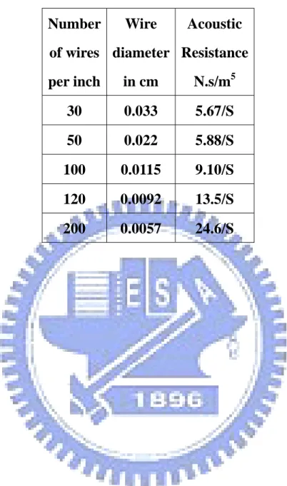
(10) LIST of TABLES Table 1.. Acoustic resistance of a screen of area S .................................................. 42. Table 2. Experimentally identified lumped-parameters of a microspeaker .............. 43 Table 3. The dimensions of the diaphragm and voice-coil assembly of the microspeaker ............................................................................................... 44 Table 4. The L9 (34 ) orthogonal array of the Taguchi method. .............................. 45. Table 5. Four weighting schemes for the cost function. ........................................... 46 Table 6. The values of the cost function in the Taguchi analysis for nine runs and four weighting schemes .............................................................................. 47 Table 7. The calculated performance parameters of sensitivity analysis and the associated cost function. ............................................................................. 48 Table 8. Resulting obtained using the constrained optimization of vented-box system ................................................................................................................... 49 Table 9. Input data of diaphragm geometry .............................................................. 50 Table 10 Output data of SPL response of microspeaker ............................................ 51 Table 11. Normalize the input and output data ........................................................... 52 Table 12. difference between target output and actual output .................................... 53 Table 13. New set of input-output pair ....................................................................... 54 Table 14. Difference of new set of microspealer performance ................................... 55 Table 15. Compare results obtained via ANSYS and NNSA ................................... 56. viii.

(11) LIST of FIGURES Fig. 1.. (a)Electro-mechano-acoustical analogous circuit of loudspeaker. (b) Same circuit with acoustical impedance reflecting to mechanical system. ..................................................................................................................... 58. Fig. 2.. The mechanical system of loudspeaker. (M is diaphragm and voice coil mass, k is stiffness of suspension, C is damping factor) ............................. 59. Fig. 3.. (a) Detailed Electro-mechano-acoustical analogous circuit of loudspeaker. (b) Another form of acoustic system. ......................................................... 60. Fig. 4.. (a) An acoustic resistance consisting of a fine mesh screen. (b) Analogous circuit. ................................................................................. 61. Fig. 5.. (a) Closed volume of air that acts as acoustic compliance. (b) Analogous circuit................................................................................... 62. Fig. 6.. (a) Cylindrical tube of air which behaves as acoustic mass. (b) Analogous circuit. ................................................................................. 63. Fig. 7.. Analogous circuit for radiation impedance on one side of circuit piston in infinite baffle. .............................................................................................. 64. Fig. 8.. (a) Perforated sheet of thickness t having holes of radius a spaced a distance (b) Geometry of the narrow slit. ................................................................. 65. Fig. 9.. (a) The model of microspeaker diaphragm with top view (b) The dimensions of diaphragm-voice coil assembly ............................ 66. Fig. 10. The finite element model and mesh including diaphragm and voice-coil (a) top view (b) bottom view ...................................................................... 67 Fig. 11. The results of the modal analysis with mode shape (a) the first piston mode (b) the second piston mode ......................................................................... 68 Fig. 12. Mechanical impedance of the diaphragm-voice coil assembly Z ms ............ 69. ix.

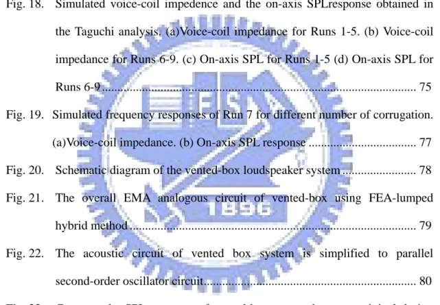
(12) Fig. 13. A frame of EBP ........................................................................................... 70 Fig. 14. Photos of a mobile phone microspeaker. (a) Front view (b) Rear view ..... 71 Fig. 15. The experimental arrangement for (a)measuring voice-coil impedance (b)measuring the on-axis SPL response .................................................... 72 Fig. 16. Simulated and measured frequency responses of the microspeaker. (a) the voice-coil impedance and (b) on-axis SPL response. ................................. 73 Fig. 17. Definitions of performance parameters of the SPL response ..................... 74 Fig. 18. Simulated voice-coil impedence and the on-axis SPLresponse obtained in the Taguchi analysis. (a)Voice-coil impedance for Runs 1-5. (b) Voice-coil impedance for Runs 6-9. (c) On-axis SPL for Runs 1-5 (d) On-axis SPL for Runs 6-9 ...................................................................................................... 75 Fig. 19. Simulated frequency responses of Run 7 for different number of corrugation. (a)Voice-coil impedance. (b) On-axis SPL response ................................... 77 Fig. 20. Schematic diagram of the vented-box loudspeaker system ........................ 78 Fig. 21. The overall EMA analogous circuit of vented-box using FEA-lumped hybrid method ............................................................................................. 79 Fig. 22. The acoustic circuit of vented box system is simplified to parallel second-order oscillator circuit..................................................................... 80 Fig. 23. Compare the SPL response of vented-box system between original design and optimal design. ..................................................................................... 81 Fig. 24. Frequency response of optima vented-box design of microspeaker (a)Voicecoil impedance (b) On-axis SPL ............................................................... 82 Fig. 25. The frame of neural network system with 4-NH-MH-3................................ 83 Fig. 26. Converge profile of SA algorithm with 4-10-6-3 NN system ..................... 84 Fig. 27. The efficiency comparison between experiment and simulation (a) experiment of microspeaker sensitivity (b) efficiency of microspeaker x.

(13) derived by four methods ............................................................................. 85 Fig. 28. Experimental arrangement for measuring sound power ............................. 86 Fig. 29. Loudspeaker efficiency comparison between experiment and simulation . 87. xi.

(14) NOMENCLATURE a = Radius of each hole of the metallic frame a1, a2, a3 = Coefficients of characteristic equation bI , bJ , bK = Bias units Bl = Electromechanical transformation ratio, namely product of magnetic flux. density and voice–coil conductor length in air gap of the loudspeaker driver b = Spaced a distance on center of each hole of the metallic frame C A = Acoustic compliance. CAB1 = Acoustic compliance of enclosure of vented-box C AF = Acoustic compliance of front cavity C AF 11 , C AF 12 = Acoustic compliance in circuit for piston air load impedance C A1 = Acoustic compliance in circuit for piston air load impedance CM = Mechanical compliance CMS = Mechanical compliance of diaphragm suspension c = Speed of sound. d ( k ) = Output training data of neural network d = the width of the outer arc of diaphragm eg = The driving voltage E(s) = Cost function for NN Feq = Unbalance force amplitude f = the excitation force delivered by the voice-coil unit f (x) = Objective function f A = Resonance of acoustical system (rad/s) f 0 = The lower cutoff frequency f1 = The upper cutoff frequency xii.

(15) H = the height of inner arc of diaphragm h = the height of outer arc of diaphragm k1, k2 = Spring constant of the rotating machine and the vibration absorber LE = Electrical inductance LP = Length of vent M A = Acoustic mass M ABP = Acoustic mass of vent. M AB1 = Acoustic mass in circuit for piston air load impedance M AFP1 , M AFP 2 = Acoustic mass of holes of the metallic frame M AF 11 , M AF 12 = Acoustic mass in circuit for piston air load impedance M AM = Acoustic mass of the metallic frame M AP = Acoustic mass of duct M A1 = Acoustic mass in circuit for piston air load impedance. M M = Mechanical mass M MD = Mechanical mass of diaphragm m1, m2 = Mass of the rotating machine and the vibration absorber N = The number of holes of the metallic frame O j = The jth output neuron of the hidden layer p ( x) = acoustic pressure of transmission line. p1 , p2 = Acoustic pressure at x = 0 and x = L p = Acceptance probabilities QA = Quality factor of the acoustic system QM = Quality factor of the mechanical system RA = Acoustic resistance. xiii.

(16) RAB1 , RAB 2 = Acoustic resistance in circuit for piston air load impedance RABP = Acoustical resistance of duct RA1 , RA 2 = Acoustic resistance in circuit for piston air load impedance. RE = Electrical resistance RE' = The eddy current losses in the magnetic circuit RM = Mechanical resistance RMS = Mechanical resistance of diaphragm suspension S D = Area of diaphragm S P = Area of duct SPL = The mean SPL in the piston bandwidth. STD = The standard deviation of SPL in the piston bandwidth T = a control parameter called the temperature T0 = Initial temperature T f = Final temperature t = Thickness of diaphragm. u , = the mean velocity of the diaphragm V = Volume of cavity VABC = Total volume of cavity VP = Volume of duct Z AB = Acoustic impedance in rear of diaphragm Z AF = Acoustic impedance in front of diaphragm Z AM = Acoustic impedance of the metallic frame Z AR1 , Z AR 2 = Acoustic radiation impedance Z A1 , Z A 2 = Partial acoustic impedance in front of diaphragm Z EB = Electrical impedance xiv.

(17) Z M , Z MS , Z ms = Mechanical impedance. α = A cooling constant Δ(ω ) = The frequency-dependent characteristic equation. μ = The kinematic coefficient of viscosity ρ = Mass ratio ρ0 = Density of air η = A constant known as the learning factor from 0 to 1 γ = A constant known as learning factor from 0 to 1 ΔE = Variation of the objective function. ω = angular frequency (rad/s). ω A = Resonance of acoustical system (rad/s) ωM = Resonance of mechanical system (rad/s) ω0 = Nature frequency of the vibration absorber system (rad/s) x ( k ) = Input training data of neural network yk = the kth output neuron of the output layer. xv.

(18) 1 Introduction Miniaturization is the trend of the 3C (computer, communication, and consumer electronics) portable devices such as mobile phones, personal digital assistants (PDAs), MP3 player, etc. Loudspeakers in these devices are required to play speech and music signals with acceptable loudness and sound quality. This demand poses a difficult problem to the design of micro-speakers whose physical sizes are usually very small. In contrast to large loudspeakers, the structures of micro-speakers are generally simplified enough with suspension removed. The diaphragm serves as not only a sound radiator but also the suspension.. Thus, the pattern design of the. diaphragm is crucial to the overall response and performance of a micro-speaker. In this paper, a hybrid approach that combines finite element analysis (FEA) and electro-mechano- acoustical (EMA) analogous circuit is presented to provide a more accurate model than the conventional approaches. In particular, the minute details of diaphragms are taken into account in calculating the mechanical impedance of the diaphragm-voice coil assembly using the FEA.. In order to meet the requirement of. output level and sound quality delivered by micro-speakers, an optimization procedure is also presented to determine the optimal pattern and dimensions of the diaphragm. Traditionally, most loudspeaker studies focused on large loudspeakers.. In. recent years, however, micro-speakers have received increased research attention owing to rapid development of 3C industries. The characteristics of micro-speakers have been studied extensively in a variety of aspects, including the structure dynamics of the diaphragm, the voice-coil impedance properties of cover perforation [1]-[4], electronic compensation [5], and structural optimization [6]. A well-known method to model of dynamic moving-coil micro-speakers is through the use of the EMA. 1.

(19) analogy.. Lumped parameter models can be established, with the aid of such. approach [7]-[9].The Thiele and Small (T-S) parameters of the micro-speaker need to be experimentally identified prior to the response simulation [10].. Using the. analogous circuit, the dynamic responses of micro-speaker can readily be simulated, enabling the ensuing design [11]. Despite the simplicity, the lumped parameter model is incapable of predicting the higher-frequency response of the micro-speaker which is strongly influenced by the diaphragm, corrugation and the enclosure.. Modeling of the flexural motion of the. diaphragm calls for more sophisticated techniques such as finite element analysis (FEA). Natural frequencies and mode shapes of the diaphragm-voice coil assembly can be calculated by FEA [12]-[14]. Kwon and Hwang [15] used FEA to examine acoustic performance of micro-speakers in lower frequency region for various designs of diaphragm.. Chao et al. [16] modeled a micro-speaker with a corrugated. diaphragm using FEA. The electromagnetic, mechanical and acoustical subsystems of the speaker were represented by a coupled FEA model. The response of three corrugation angles of 15°, 45°, and 75° were investigated. FEA is employed in this paper to model the diaphragm of micro-speaker. However, a feature of this work that differs itself from the previous studies is that the FEA model of the diaphragm is modified into a lumped-parameter model, where mechanical impedance of the diaphragm-voice coil assembly is obtained using harmonic analysis of the FEA model. This facilitates tremendously the coupling of the diaphragm model with the models of the rest of the system such as an acoustical enclosure that is usually represented by a lumped-parameter model.. Using this simulation platform, the voice-coil impedance. and the on-axis sound pressure level (SPL) of the micro-speaker can be calculated by solving the loop equations [17] of the coupled EMA analogous circuit. Another feature of the thesis is that the aforementioned hybrid FEA-lumped 2.

(20) parameter model is introduced to extend the design optimization developed in Ref. [6]. The diaphragm pattern is optimized using the Taguchi method [18], [19].. In. addition, the optimal number of diaphragm corrugation is determined via sensitivity analysis. A number of performance measures concerning the lower cutoff frequency ( f 0 ), the upper cutoff frequency ( f1 ), mean SPL in the piston range, and the flatness of SPL response are weighted and summed to constitute the cost function. Using the best result of the Taguchi analysis as initial condition, sensitivity analysis is then carried out to determine the number of corrugations for the diaphragm. The thus found optimal design will be compared with the non-optimal design in this thesis. Predication of the micro-speaker performance poses a complex non-linear problem as the system integrates the diaphragm geometry and performance of micro-speaker produced via FEA-lumped parameters model. In this thesis an alternative artificial neural network approach is developed to predict the performance of micro-speaker when the diaphragm geometry data is input. A set of the diaphragm geometry as inputs and the corresponding micro-speaker performance as outputs (the lower cutoff frequency ( f 0 ), mean SPL in the piston range, and the flatness of SPL response) are utilized to train the network. The results predicted by the models are in good agreement with the simulation data, and the average deviations for all the cases are well within ±5%. Another optimal approach of diaphragm employs the neural network and simulated annealing (NNSA), and consists of two stages. Stage 1 formulates an objective function like as the aforementioned Taguchi method for a problem using a neural network method to predict the value of the response for the given input parameters setting. Stage 2 applies the simulated annealing algorithm to search for the optimal parameter combination. The purpose of the present study is to exploit nonlinear function approximation capability of a neural network to develop a simple 3.

(21) yet efficient hybrid optimization strategy by combining a multilayer feedforward neural network with a Simulated Annealing algorithm.. 4.

(22) 2 Theory and Method A loudspeaker is an electroacoustic transducer that converts the electrical signal to sound signal. The processes of the transduction are complex. These cover the electrical, mechanical, and acoustical transduction. In order to model the process of the transduction, the EMA analogous circuit can be used to simulate the dynamic behavior of the loudspeaker. The circuit is overall and decomposed to electrical, mechanical, and acoustic part. A loudspeaker is characterized by a mixed of electrical, mechanical, and acoustical parameters.. 2.1 Electrical-mechanical-acoustical analogous circuit The concept of the electric circuit often applied to analyze transducers in the electrical and mechanical system. The technique analysis of the electric circuit can be adopted to analyze the transduction of the mechanical and acoustical system. The simple diagram of EMA analogous circuit is shown in Fig. 1. The subject of EMA analogous circuit is the application of electrical circuit theory to solve the coupling of the electrical, mechanical and acoustical system. The EMA analogous circuit is formulated by the differential equations of the electrical, mechanical, and acoustical system and the differential equations can be modeled by the circuit diagram. The rules of analytic methods are follows. For the electromagnetic loudspeaker, the diaphragm is driven by the voice coil. The voice coil has inductance and resistance which are defined RE and LE . The term RE and LE are the most common description of a loudspeaker’s electrical impedance. In order to model the nonlinearity of inductance, a resistance RE′ can be parallel connected to inductance. Thus, the electrical impedance of loudspeaker is formulated as:. Z E = RE + ( jω LE // RE′ ). (1). When the current (i) is passed through the voice coil, the force ( f ) is produced. 5.

(23) and that drives the diaphragm to radiate sound. The voltage (e) induced in the voice coil when it movies with the mechanical velocity (u) . The basic electromechanical equations that relate the transduction of the electrical and mechanical system are listed.. f = Bli. (2). e = Blu. (3). Here, electro-mechanical transduction can be modeled by a gyrator. So, the loudspeaker impedance is formulated as:. Z=. e Bl 2 = ZE + i Z M + Z MA. (4). where Z M is the mechanical impedance and Z MA is the acoustical impedance reflecting in mechanical system as shown in Fig. 1(b). A simple driver model is shown in Fig. 2. This simple driver model can be used to describe the mechanical dynamics of the electromagnetic loudspeaker. Force f is produced according to the Eqs. (2). Vibration of the diaphragm of the loudspeaker displaces air volume at the interface. The primary parameters of the simple driver are the mass, compliance (compliance is the reciprocal of stiffness) and damping in the mechanical impedance. The acoustical impedance is induced by the radiation impedance, enclosure effect and perforation of the enclosure. f S is the force that air exerts on the structure. The coupled mechanical and acoustical systems can be simplified as :. M MD && x= f −. x − RMS x& − f S CMS. (5). where M MD is the mass of diaphragm and voice coil, f is the force in newtons,. f S is the force that air exert on the structure, CMS is the mechanical compliance, RMS is the mechanical resistance and x is the displacement.. 6.

(24) M MD ( s )( jω ) 2 x( s ) = f ( s ) − M MD ( s ) jωu ( s ) = f ( s ) −. x( s) − RMS jω x( s ) − f S (6) CMS. u ( s) − RMS u ( s ) − f S jωCMS. f = ( Z M + Z A )u ( s ) where Z M = jω M MD + RMS +. (7). 1 is the mechanical impedance and Z A is the jωCMS. acoustical impedance. f S = Z Au. (8). The acoustical impedance primarily includes radiation impedance, enclosure impedance, and perforation of the enclosure.. The acoustical impedance can be. formulated as: Z A = Z AF + Z AB. (9). The general acoustic circuit is shown in Fig. 3(a). The Z AF means the impedance in the front of diaphragm and Z AB means that in the back side. In general, the circuit would turn to Fig. 3(b) the general form in the electronics. The following discussion will use this kind of circuit. The two basic variables in acoustical analogous circuit are pressure p and volume velocity U . Because of using impedance analogy, the voltage becomes pressure p and current becomes volume velocity U . Therefore, the ground of this circuit showing in Fig. 3 means the pressure of the free air. Thus, it also can employ the concept about the mechanical system and the acoustical system can be coupled by the below two equations. fS = SD p. (10). U = S Du. (11). The equation. f S = S D p represents the acoustic force on the diaphragm. generated by the difference in pressure between its front and back side, where D S is the effective diaphragm area and p is the difference in acoustic pressure across the 7.

(25) diaphragm. The volume velocity source U=SDu represents the volume velocity emitted by the diaphragm. From the Eqs. (10), the pressure difference between the front and rear of the diaphragm is given by p = U ( Z AF + Z AB ). (12). Using Eqs. (10) and (11), force field can be transformed to pressure field.. 2.2 The method of parameter identification Almost all of the useful loudspeaker parameters had been defined by other researchers before Thiele and Small.. However, Thiele and Small made these. parameters in a complete design approach and shown how they could be easily determined from impedance data. There are at least four methods for measuring Thiele and Small parameters from driver impedance data. They are: 1. Closed box (Delta compliance method) 2. Added mass (Delta mass method) 3. Open box only 4. Open box/closed box The first two procedures are the most popular. But for miniature speaker, the closed box method is the best choice. The closed box method and curve fitting method are adopted to calculate the Thiele and Small parameters. Placing the driver in a closed box will induce the alteration of the resonant frequency. The curve fitting employs the impedance of system to calculate the parameters of Thiele and Small precisely. Both methods are explained in the following section.. Curve fitting method The curve fitting method is used to calculate QES and the result is more accurate. The procedure of the curve fitting method is explained as follows.. 8.

(26) (a) Choose the (. 1 1 jω M + R + jωC. ) to be become the basic element that it fit a. peak of the impedance curve. Because the purpose of the method is to fit the mechanical part, the electrical part can be obtained previously. (b) Choose the fitting range in the impedance curve. If the range of the impedance curve is chosen broadly, result of the fitting is poor. Therefore, the range that starts and ends both sides of peak enclosures the peak, and it can be chosen. Then, the peak will fit better and it is obtained second order system transfer function. (c) We compare the coefficient between the second order transfer function and 1 s + 2ξωs + ωs 2 2. , then the parameters ωs and QMS are solved.. ωs = 2π f S QMS =. 1 2ξ. QES = QMS (. (13) RE ) RES. (14). Closed box method When the impedance of a mechanical system is Z M = jω M MS + RMS + resonant frequency is ωs =. 1 M MD CMS. 1 the jωCMS. . When a driver is placed in a closed box, its. resonant frequency rises. This is because the inward cone motion is resisted not only by the compliance of its own suspension, but also by the compression of the air in box. The compliance of the driver suspension is reduced by the compliance of the air spring. If the total compliance has decreased, the resonant frequency of the driver will rise. The concept can employed to calculate to the mechanical mass, mechanical compliance and mechanical resistance of the system. The closed box procedure for determining T/S parameters is given below: 9.

(27) 1. Measure f S and QES using the curve fitting method 2. Mount the driver in the test box. Make sure there are no air leaks around the box and speaker. One point must be noticed is that the testing volume for the case of miniature speaker must be less than 0.015L, or you can’t measure the realizable T/S parameters. 3. Measure the new in-box resonant frequency and electrical Q using the same procedure as that used in step 1. Label these new value fC and QEC . 4. Compute the VAS as follows: VAS = VT (. f C QEC − 1) Where VT is the total volume of the tested box f S QES. Therefore, the mechanical mass M MD and mechanical compliance CMS can be solved as CMS =. VAS ρ0c 2 S D2. (15). M MS =. VAS ωS2CMS. (16). M MD = M MS − 2M 1. (17). where M 1 is the air-load impedance at low frequency. On the other hand, the parameters, and the mechanic resistance ( MS R ) and the motor constant ( Bl ) can be calculated, using the following formula: RMS = Bl =. ωS M MS. (18). QMS. ωS RE M MS. (19). QMS. And the lossy voice-coil inductance can be calculated, using the following method: Z E ( jω ) ≈ ( jω ) n LE. ⎡ ⎤ n ⎡ ⎤ n −1 Le Le RE' = ⎢ ω , LE = ⎢ ⎥ ⎥ω ⎣ cos(nπ / 2) ⎦ ⎣ cos(nπ / 2) ⎦ (n=1:inductor;n=0:resistor) 10. (20).

(28) The parameters n and Le can be determined from one measurement of ZVC at a frequency well above f s , where the motional impedance can be neglected Z E = ZVC − RE n=. Z ⎡ Im( Z E ) ⎤ ln Z 2 − ln Z1 1 tan −1 ⎢ ， LE = En ⎥= 90 ω ⎣ Re( Z E ) ⎦ ln ω2 − ln ω1. (21). The method to calculate lossy voice-coil inductance is described [20].. 2.3 Modeling Acoustical Systems Electroacoustics is using the analogous circuit to model the acoustical behavior including acoustic mass, acoustic resistance and acoustic compliance. The impedance type of analogy is the preferred analogy for acoustical circuits. The sound pressure is analogous to voltage in electrical circuits. The volume velocity is analogous to current.. Acoustic Resistance Acoustic resistance is associated with dissipative losses that occur when there is a viscous flow of air through a fine mesh screen or through a capillary tube. Fig. 4(a) illustrates a fine mesh screen with a volume velocity U flowing through it. The pressure difference across the screen is given by p = p1 − p2 , where p1 is the pressure on the side that U enters and p2 is the pressure on the side that U exits. The pressure difference is related to the volume velocity through the screen by p = p1 − p2 = RAU. (22). where RA is the acoustic resistance of the screen. The circuit is shown in Fig. 4(b). Theoretical formulas for acoustic resistance are generally not available. The values are usually determined by experiments. Table 1 gives the acoustic resistance of typical screens as a function of the area S of the screen, the number of wires in the screen, and the diameter of the wires.. 11.

(29) Acoustic compliance Acoustic compliance is a parameter that is associated with any volume of air that is compressed by an applied force without an acceleration of its center of gravity. To illustrated an acoustic compliance, consider an enclosed volume of air as illustrated in Fig. 5(a). A piston of area S is shown in one wall of the enclosure. When a force f is applied to the piston, it moves and compresses the air. Denote the piston displacement by x and its velocity by u . When the air is compressed, a restoring force is generated which can be written f = kM x , where kM is the spring constant. (This assumes that the displacement is not too large or the process cannot be modeled with linear equation.) The mechanical compliance is defined as the reciprocal of the spring constant. Thus we can write x 1 = udt CM C M ∫. f = kM x =. (23). This equation involves the mechanical variables f and u . We convert it to one that involves acoustic variables p and U by writing f = pS and u = U / S to obtain p=. 1 1 Udt = Udt ∫ S CM CA ∫. (24). 2. This equation defines the acoustic compliance C A of the air in the volume. It is given by C A = S 2 CM. (25). An integration in the time domain corresponds to a division by jω for phasor variable. It follows from Eqs. (24). That the phasor pressure is related to the phasor volume velocity by p = ZA =. U . Thus the acoustic impedance of the compliance is jωC A. p 1 = U jwC A. (26). The impedance which varies inversely with jω is a capacitor. The analogous circuit 12.

(30) is shown in Fig. 5(b). The figure shows one side of the capacitor connected to ground. This is because the pressure in a volume of air is measured with respect to zero pressure. One node of an acoustic compliance always connects to the ground node. The acoustic compliance of the volume of air is given by the expression derived for the plane wave tube. It is V ρc2. CA =. (27). Acoustic mass Any volume of air that is accelerated without being compressed acts as an acoustic mass. Consider the cylindrical tube of air illustrated in Fig. 6(a) having a length l and cross-section S . The mss of the air in the tube is. M0. M M = ρ0 Sl . If. the air moved with velocity u , the force required is given by f = M M du. dt. . The. volume velocity of the air through the tube is U = Su and the pressure difference between the two ends is p = p1 − p2 = f. S. . It follows from these relations that the. pressure difference p can be related to the volume velocity U as follows:. p = p1 − p2 =. M M du M M dU dU = 2 = MA S dt S dt dt. (28). where M A is the acoustic mass of the air in the volume that is given by. MA =. M M ρ0l = S2 S. (29). A differentiation in the time domain corresponds to a multiplication by jω for sinusoidal phasor variable. If follows from Eqs. (28) that the phasor pressure is related to the phasor volume velocity by p = jω M AU . Thus the acoustic impedance of the mass is. ZA =. p = jω M A U. (30). An electrical impedance which is proportional to jω is an inductor. The analogous circuit is shown in Fig.. 6(b). For a tube of air to act as a pure acoustic 13.

(31) mass, each particle of air in the tube must move with the same velocity. This is strictly true only if the frequency is low enough. Otherwise, the motion of the air particles must be modeled by a wave equation. An often used criterion that the air in the tube act as a pure acoustic mass is that its length must satisfy l ≤ λ. 8. , where λ is the. wavelength.. Radiation impedance of a baffled rigid piston Radiation impedance can be easily explained by an example of the diaphragm vibration. When the diaphragm is vibrating, the medium reacts against the motion of the diaphragm. The phenomenon of this can be described as there is impedance between the diaphragm and the medium. The impedance is called the radiation impedance. The detail of the theory of radiation impedance is clearly described by Bernek. The analogous circuit of the radiation impedance for the piston mounted in an infinite baffle is shown in Fig. 7. The acoustical radiation impedance for a piston in an infinite baffle can be approximately over the whole frequency range by the analogous circuit. The parameters of the analogous values are given by. M A1 =. 8ρ0 3π 2 a. (31). RA1 =. 0.4410 ρ0 c π a2. (32). RA 2 =. ρ0c π a2. (33). C A1 =. 5.94a 3 ρ0c 2. (34). where ρ0 is the density of air, c is the sound speed in the air, a is the radius of the circuit piston.. Radiation impedance on a piston in a tube The flat circuit piston in an infinite baffle that is analyzed in the preceding 14.

(32) section is commonly used to model the diaphragm of a direct-radiator loudspeaker when the enclosure is installed in a wall or against a wall. If a loudspeaker is operated away from a wall,. the acoustic impedance on its diaphragm changes. It is not. possible to exactly model the acoustic radiation impedance of this case. An approximate model that is often used is the flat circuit piston in a tube. The analogous circuit for the piston in a long tube is the same from as that for the piston in an infinite baffle; only the element values are different. The analogous circuit is given in Fig. 7. The parameters of the analogous values are given by 0.6133ρ πa. (35). RA1 =. 0.5045ρ c π a2. (36). RA 2 =. ρc π a2. (37). C A1 =. 0.55π 2 a 3 ρ c2. (38). M A1 =. Other acoustic elements Perforated sheets are often used as an acoustic resistance in application where an acoustic mass in series with the resistance is acceptable. Fig. 8(a) illustrates the geometry. If the holes in the sheet have centers tat are spaced more than on diameter apart and the radius a of the holes satisfies the inequality 0.01. f. < a < 10. f. ,. where f is the frequency and a is in m, the acoustic impedance of the sheet is given by ZA =. ⎡t ⎛ π a 2 ⎞⎤ ρ0 ⎧⎪ ⎡ ⎛ a ⎞ ⎤ ⎫⎪ u j t ω ω 2 2 1 1.7 + − + + ⎨ ⎢ ⎥ ⎜ ⎟ ⎜1 − ⎟ ⎥ ⎬ ⎢ 2 N π a 2 ⎩⎪ a b b ⎠ ⎦ ⎭⎪ ⎝ ⎣ ⎝ ⎠⎦ ⎣. (39). where N is the number of holes. The parameters μ is the kinematic coefficient of viscosity. For air at 20° C and 0.76 mHg , μ ≈ 1.56 × 10−5 m. 15. 2. s. . This parameter.

(33) 1.7 value approximately as T. , where T is the Kelvin temperature and P0 is the. P0. atmospheric pressure. A tube having a very small diameter is another example of an acoustic element which exhibits both a resistance and a mass. If the tube radius a in meters satisfies the inequality a < 0.002. ZA =. f. , the acoustic impedance is given by. 4ρ l ' 8η l + jω 0 2 4 πa 3π a. (40). where l is the actual length of the tube and l ' is the length including end corrections.. parameter η. The. η = 1.86 ×10−5 N ⋅ S. m2. is. the. viscosity. coefficient.. For. air,. at 20° C and 0.76 mHg . This parameter varies with. temperature as T 0.7 , where T is the Kelvin temperature. If the radius of the tube satisfies the inequality 0.01. ZA =. f. < a < 10. , the acoustic impedance is given by. f. ρ0 ρ l' ⎛l ⎞ 2ωu ⎜ + 2 ⎟ + jω 0 2 2 πa πa ⎝s ⎠. For a tube with a radius such that 0.002. f. < a < 0.01. (41). f. , interpolation must be. used between the two equations. A narrow slit also exhibits both acoustic resistance and mass. Fig. 8(b) shows the geometry of such a slit. If the height t of the slit in meters satisfies the inequality t < 0.003. f. , the acoustic impedance of the slit, neglecting end corrections. for the mass term, is given by. ZA =. 12η l ρl + jω 0 3 tω 5ωt. (42). 2.4 Finite Element Analysis of the Diaphragm-Voice coil Assembly The FEA is applied to model the diaphragm-voice coil assembly shown in Figs.9(a)-(b) with dimensions summarized in Table 2.. The material properties of the. diaphragm-voice coil assembly are included in Table 3. The FEA is conducted using 16.

(34) ANSYS® [21], where the element “shell 63” is used. The shell element has four nodes and 6 degrees of freedom (Ux, Uy, Uz, ROTx, ROTy, ROTz) at each node.. The. finite element model and the mesh of the diaphragm with voice-coil are shown in Figs. 10 (a)-(b). The boundary conditions are selected that all degrees of freedom for the outer rim of the diaphragm and the X, Y-displacements of the voice-coil are set to zero. The fundamental resonance frequency calculated by the modal analysis is 803 Hz and the associated mode shape is shown in Fig. 11 (a). The fundamental mode known as the piston mode can be used to “fine-tune” FEA parameters to match the measured data.. The measured result of the fundamental resonance frequency is 792 Hz which. is about 1.4 % lower than the FEA prediction. Figure 11 (b) shows another higher order mode at 18978 Hz, where major motion takes place at the center circular portion inside the voice-coil bobbing, while the outer ring of the diaphragm is almost motionless.. Due to this nature, we call it the second piston mode.. The SPL. response shows a peculiar boost above the second piston mode, as will be seen in the experimental results. In order to fit the aforementioned FEA model into the analogous circuit of the microspeaker system, the dynamics of the FEA model has to be adapted into a lumped parameter model next. To begin with, the short-circuit mechanical impedance ( Z ms ) defined in the following expression is calculated using the FEA harmonic analysis:. Z ms =. f , u. (43). where u denotes the mean velocity of the diaphragm and f is the excitation force delivered by the voice-coil unit.. f = Bli. (44). To calculate Z ms , the excitation force is set to be 0.13 N. The damping ratio is assumed to be 0.16 and 0.07 for 20 ~ 4000 Hz and for 4k ~ 20 kHz, respectively.. 17.

(35) The complex displacements calculated using the FEA harmonic analysis are then converted into the average velocity ( u ).. Using Eq. (43), the mechanical impedance. of the diaphragm-voice coil assembly Z ms can be calculated, as shown in Fig. 12. As a result, the dynamics of the flexible diaphragm is represented by a frequency-dependent impedance element and is readily integrated into the analogous circuit.. 2.5 Neural networks Artificial neural network [22] [23] is a system which is deliberately constructed to make use of some organizational principles resembling those of the human brain. ANN has a large number of highly interconnected processing elements (nodes or units) that usually operate in parallel and are configured in regular architectures. A processing element (PE) can dynamically respond to its inputs stimulus, and the response completely depends on its local information that the input signals arrive at the PE via impinging connections and connection weights. It has the ability to learn , recall and generalize from training data by assigning or adjusting the connection weights. This thesis utilizes the error back-propagation network (EBP) which is trained by supervised learning rules. The correct output data called target vector is known compulsorily through the training cycle. Given a training set of input-output pair ( x ( k ) , d ( k ) ) , the algorithm provides a procedure for changing the weights in EBP to classify the given input patterns correctly. EBP performs two phases of data flow. First, the input pattern x ( k ) is propagated from the input layer to the output layer and as a result of this forward flow of data, it produces an actual output y ( k ) . Then the error signals resulting from the difference between. d (k ). and. y(k ). are. back-propagated from the output layer to the previous layers for them to update their weight. If the error is lower than previous setting range of allowance, the work is. 18.

(36) completed. Otherwise, repeat the above-mentioned method until the error is converged.. 2.5.1 Error Back-Propagation Network (EBP) EBP. is. multilayer. feed-forward. neural. network. (FFNN). with. the. back-propagation learning algorithm which is including input layer, hidden layer and output layer. The way of this operating is transmitting the input signal forward to the hidden layer through the calculating of activation function and then estimates from the hidden layer to the output layer. Fig13 is shown as a general FFNN figure. Every big circle is considered a neuron consisting of summer and TF (f1 or f2). The input target is shown as. x = ( x1 x2 ...... xi .... xI ). (45). and output target is shown as. d = (d1 d 2 ...... d k .... d K ). (46). O j is the jth output neuron of the hidden layer. yk is the kth output neuron of the output layer. The points in front of TF= f1 and f2 are considered as m j and. nk respectively. yk = f 2 (nk ) ，k = 0,1,........, K. (47). nk = wk1O1 + ⋅⋅⋅⋅ + wkj O j + ⋅⋅⋅⋅ + wKJ OKJ ，k = 0,1,........, K. (48). We define the cost function as. Ek =. ( d k − yk ) 2 k=0, 1,….., K 2. (49). Then according to the gradient-descent method, the least value of Ek is estimated by ∂Ek / ∂wkj = (∂Ek / ∂yk )(∂yk / ∂nk )(∂nk / ∂wkj ) = −ek f 2 '(nk )O j. (50). ek = d k - yk. (51). assuming δ k =ek f 2 '(n k ) , the weights of the output layer are updated by 19.

(37) wkj ,new =wkj ,old + Δwkj. (52). Δwkj =ηδ k O j. (53). η is a constant known as the learning factor from 0 to 1. In Fig13 it is observed that the influence of weight v ji will extend to all output. Hence we need all the value of errors. {e1 , e2 , ⋅⋅⋅, ek , ⋅⋅⋅, eK }. . To obtain the optimum value of v ji we should calculate. the value of ∂E / ∂v ji using chain rule. ∂E / ∂v ji = (∂E / ∂y1 )(∂y1 / ∂n1 )(∂n1 / ∂O j )(∂O j / ∂m j )(∂m j / ∂v ji ) + ⋅⋅⋅ +(∂E / ∂yk )(∂yk / ∂nk )(∂nk / ∂O j )(∂O j / ∂m j )(∂m j / ∂v ji ) + ⋅⋅⋅ +(∂E / ∂yK )(∂yK / ∂nK )(∂nK / ∂O j )(∂O j / ∂m j )(∂m j / ∂v ji ) = −e1 f 2' (n1 ) w1 j f1' (m j ) xi − ⋅⋅⋅. (54). − ek f 2' (nk ) wkj f1' (m j ) xi − ⋅⋅⋅ − eK f 2' (nK ) wKj f1' (m j ) xi ⎧K ⎫ = − ⎨∑ [ek f 2' (nk ) wkj ] f1' (m j ) xi ⎬ ⎩ k =1 ⎭ K. Assuming δ jH =f1'(m j )∑ [δ k wkj ] , the above symbol H is expressed as δ in the k =1. hidden layer, and δ k is part of the output layer.. v ji ,new = v ji ,old + Δv ji. (55). Δv ji = γδ jH ( xi ) , γ is a constant known as learning factor from 0 to 1. In general, γ. is equal to η .. 2.6 Simulation Annealing Simulated annealing (SA) is a generic probabilistic meta-algorithm for the global optimization problem, namely locating a good approximation to the global optimum of a given function in a large search space. SA has demonstrated to be a good technique for solving hard combinatorial optimization problems. In SA method, each. 20.

(38) point of the search space is analogous to a state of some physical system, and the objective function E(s) to be minimized is analogous to the internal energy of the system in that state. The goal is to bring the system from an initial state to a new state with the minimum possible energy.. 2.6.1 Acceptance probabilities There are two conditions about accepting rule of SA. One is that the value of the objective function is decreased. When the value of the objective function is increased the other accepts moves with probability. p=e. − ( ΔE ). T. (56). where ΔE denotes variation of the objective function, T is a control parameter called the temperature . Next, a random number generated uniformly on the interval (0,1) is sampled, and if the sample is less than p the move is accepted. It follows that the system may move to the new state even when it is worse than the current one. It is this feature that prevents the method from staying in a local minimum—a state that is worse than the global minimum, but better than any of its neighbors. Initially the high temperature T causes the high probability of accepting a move that increases the objective function. When the search progresses the temperature is gradually decreased. Finally, the probability of accepting a move that increases the objective function becomes vanishingly small. In general, the temperature is lowered in accordance with an annealing schedule.. 21.

(39) 2.6.2 Cooling course The most generally employed annealing schedule is called exponential cooling which begins at some initial temperature T0 and decreases the temperature in steps according to. Tk +1 = α Tk. (57). where 0 < α < 1 a cooling constant. Typically, a fixed number of moves must be accepted at each temperature before proceeding to the new state. A course of SA action is stopped either when the temperature reaches some final value T f or the system is not transformed to a new state after some times. A good value for α suggested experientially is 0.95 and that T0 should be chosen so that the initial acceptance probability is higher than 0.8. The initial solution is generated typically at random.. 22.

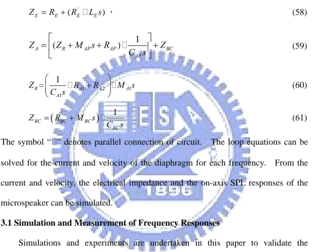
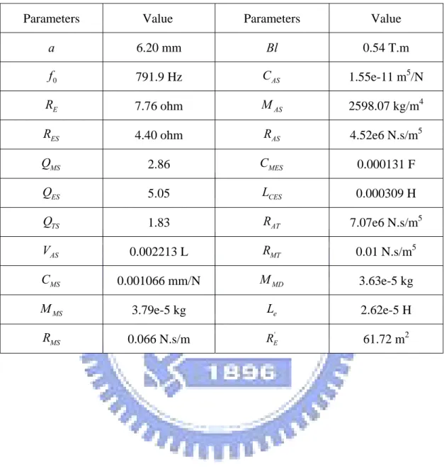
(40) 3. Design optimization of diaphragm pattern Model of microspeakers Traditionally, lumped parameters methods with EMA analogy are commonly exploited to model loudspeakers. Despite the simplicity, the conventional methods are applicable to model the dynamics in low frequency regime especially in the neighborhood of fundamental resonance. However, this may not be sufficient for microspeaker analysis. The lumped parameter model can not predict well the high frequency responses of microspeakers that may play an important role in overall performance such as output level and roll-off frequency.. In this work, the. diaphragm-coil assembly of microspeaker will be modeled using FEA. The FEA model will be combined with the EMA analogous circuit to establish a fully coupled model for the microspeaker.. EMA analogous circuit of microspeaker A sample of moving-coil microspeaker with a 16.4 mm diameter and 4.3 mm thickness is shown in Fig. 14. The front and rear view of the microspeaker are shown in Figs. 14 (a) and (b), respectively. The EMA analogous circuit of this microspeaker can be established in Fig. 3. The coupling of the electrical domain and the mechanical domain is modeled by a gyrator, whereas the coupling of the mechanical domain and the acoustical domain is modeled by a transformer [9]. The T-S parameters can be identified via electrical impedance measurement [9] and [10], as summarized in Table 2.. The dynamic response of the microspeaker can be. simulated on the platform of this model. Loop equations can be written for the preceding FEA-lumped parameter circuit of the microspeaker as follows [29]:. 23.

(41) ⎡ZE ⎢ Bl ⎢ ⎢⎣ 0. Bl − Z ms −S D Z A. 0 ⎤ ⎡ i ⎤ ⎡eg ⎤ − pD ⎥⎥ ⎢⎢ u ⎥⎥ = ⎢⎢ 0 ⎥⎥ , pD ⎥⎦ ⎢⎣ S D ⎥⎦ ⎢⎣ 0 ⎥⎦. (58). where i is the current, u is the mean velocity of the diaphragm, S D is the effective area of the diaphragm, eg is the driving voltage, s = jω is the Laplace variable, and. Z E = RE + ( RE'. LE s ) ，. (58). ⎡ 1 ⎤ Z A = ⎢( Z R + M AP s + RAP ) ⎥ + Z BC C AF s ⎦ ⎣. (59). ⎛ 1 ⎞ ZR = ⎜ RA1 + RA 2 ⎟ M A1s ⎝ C A1s ⎠. (60). Z BC = ( RBC + M BC s ). 1. (61). CBC s. The symbol “ ” denotes parallel connection of circuit. The loop equations can be solved for the current and velocity of the diaphragm for each frequency. From the current and velocity, the electrical impedance and the on-axis SPL responses of the microspeaker can be simulated.. 3.1 Simulation and Measurement of Frequency Responses Simulations and experiments are undertaken in this paper to validate the aforementioned integrated micro-speaker model. The frequency response from 20 Hz to 20 kHz of the micro-speaker is measured using a 2 Vrms sweep sine input. Figure 15 (a) shows the experimental arrangement for measuring voice-coil impedance (with symbols defined in the figure): Z vc =. es R eg − es. (62). Figure 15 (b) shows the experimental arrangement for measuring the on-axis SPL response by using a microphone positioned at 5 cm away from the micro-speaker.. 24.

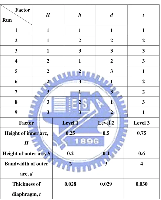
(42) Next, simulation of the diaphragm response was carried out using the integrated FEA-lumped parameter model mentioned above. Figures 16 (a) and (b) compare the voice-coil impedance and the on-axis SPL obtained from the simulation and the experiment, respectively. It can be observed that response predicted by conventional lumped parameter model is in good agreement with the measurement in low frequencies.. In high frequencies, the conventional approach fails to capture the. response due to the flexural modes of the diaphragm.. However, the response. simulated by the integrated FEA-lumped parameter model matches the measured response quite well.. 3.2 Diaphragm Optimization using the Taguchi method As mentioned previously, the diaphragm pattern has major impact on the micro-speaker response. To pinpoint the optimal pattern design, the Taguchi method and sensitivity analysis are exploited in this study. The Taguchi method [18] is very useful for experimental design, particularly for problems with finite number of discrete levels of design factors and thus reduction of the number of experiments is highly desired. In the following, the dimensions of diaphragm-voice coil assembly of micro-speakers will be optimized by using the Taguchi method. Table 4 shows the L9 (34 ) orthogonal array to be used in the Taguchi procedure.. Here, nine. observations and four factors are involved. The factors, each discretized into three levels, include the height of inner arc (H), the height of outer arc (h), the bandwidth of outer arc (d) ,and the thickness of diaphragm (t), as summarized in Table 4. The following procedure aims to find the optimal parameters for the micro-speaker diaphragm design according to the cost function:. fc = −. Δf 0 Δf Δ SPL ΔSTD × w1 + 1 × w2 + × w3 − × w4 , f0 f1 STD SPL. 25. (63).

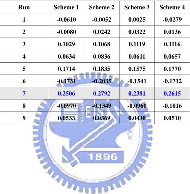
(43) where f 0 is the lower cutoff frequency of micro-speaker, f1 is the upper cutoff frequency of micro-speaker, SPL denotes the mean SPL in the piston bandwidth (defined in Fig. 17) and STD denotes the standard deviation of SPL in the piston bandwidth that serves as a flatness measure STD =. (. n 1 ∑ S P Li − S P L n − 1 i =1. ). 2. ,. (64). where n is the number of frequency components of SPL in the band and SPLi is the. ith SPL in the band. The symbol Δ signifies the difference of the performance parameters. between. the. original. design. and. the. Taguchi. design,. e.g.,. Δf 0 = f 0,Taguchi − f 0,original , w j , j = 1 ~ 4 , is the weight for the performance parameter i. In order to accommodate more design objectives, we consider using four kinds of weighting schemes, and summarized in Table 5. In scheme 1, the weights for the performance parameters are equal. Larger weights are used to emphasize the lower cutoff frequency and the mean of SPL in evaluating schemes 2 and 3, respectively. In the weighting scheme 4, however, more emphasis is placed on the lower cutoff frequency, the upper cutoff frequency and the mean of SPL than the standard deviation of SPL. Figures 18 (a)-(d) show the simulated voice-coil impedance and the SPL response of Run 1 to 9 in the L9 (34 ) orthogonal array. The values of calculated cost function for all weighting schemes are summarized in Table 6.. The cost. function of Run 7 has attained the highest value among all schemes. In Run 7, the lower cutoff frequency is reduced to 567.3 Hz, the upper resonance frequency is increased to 20 kHz, the SPL of the resonance frequency is increased to 84.8 dB, and the standard deviation is 1.88 dB. The optimal design result indicates that the height of inner arc (H) and the width of the outer arc (d) should be as large as possible, and 26.

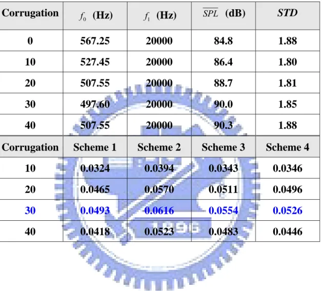
(44) the height of outer arc (h) should be as small as possible, which will maximize the cost functions.. 3.3 Sensitivity Analysis of Corrugation Sensitivity analysis of diaphragm corrugation is undertaken to examine the effect of corrugation number on the micro-speaker performance. The analysis is based on the optimal diaphragm dimensions obtained in Run 7 of the preceding Taguchi procedure. The simulated voice-coil impedance and SPL response of Run 7 for different corrugation numbers are shown in Figs. 19 (a)-(b).. The values of. performance indices and the resulting cost function for different corrugation numbers are summarized in Table 7. It can be observed that corrugation tends to reduce the fundamental resonance frequency, but the relation is not linear. Further, corrugation tends to increase the mean and the standard deviation of the SPL response. In another word, increasing the number of corrugations will decrease the flatness of SPL during the effective frequency range. Nevertheless, the corrugation does not seem to affect the upper cutoff frequency significantly. The values of cost function in relation to the corrugation number for different weighting schemes are also summarized in Table 7. The values of cost function are derived from the result of Run 7 of the Taguchi method. The results reveal that the optimal corrugation number is 30, in which the cost function is within 0.0493 - 0.0616 for the four weighting schemes.. 27.

(45) 4. Bass-enhancement and Optimization Using FEA-Lumped In this section, the simulation of the vented-box system designed to enhance the bass response of the micro-speaker is carried out using the integrated FEA-lumped parameter model mentioned above.. This will be explored in a more general context. of vibration absorber theory. In this paper, vibration absorber theory will not be discussed. The detail is clearly discussed in [28]. Next, the Sequential Quadratic Programming (SQP) suggested in References [24]-[27] is utilized to design the optimized vented-box system.. 4.1 Modeling the Vented-box Acoustical System The general diagram of a vented-box system is shown in Fig. 20 The system primarily consists of an enclosure of volume VAB and a port with a cross-sectional area. SP with radius aP and length LP. The mechanism of low-frequency enhancement lies in the Helmholtz resonator comprised of the acoustic mass in the vent and the acoustic compliance in the enclosure. More precisely, the vent can be modeled as an acoustic mass and an acoustic resistance. The acoustic resistance and acoustic mass of the port, and acoustic compliance of the enclosure are given by [9] RABP =. ⎡L ⎤ ρ0 2ωμ ⎢ P + 2 ⎥ 2 π aP ⎣ aP ⎦. M ABP = C AB =. ρ0 SP. (65). LP .. (66). VAB ρ0c 2. (67). The mechanical impedance obtained using FEA mentioned above is changed into a lumped-parameter model. Therefore, the overall EMA analogous circuit of vented-box is shown in Fig. 21.. 4.2 Optimal Design of the Vented-box The design variables are selected to be the port radius ( aP ), the duct length ( LP ) 28.

(46) and the volume of cavity ( VABC ).. The Helmholtz frequency of the vented box. system is selected to be 400Hz.. To initiate the SQP constrained optimization. procedure, the lower resonance frequency of the coupled speaker-enclosure system is also selected to be 400 Hz. The design variables are selected to be the port radius, the duct length and the volume of cavity.. To make circuit like as a parallel. second-order oscillator circuit, the acoustic system is simplified to Fig. 22. And the cost function is chosen as the maximum sound pressure level at the frequency 400Hz. This can be written in terms of the following optimization formalism: ⎧ 0.001 ≤ aVP ≤ 0.2 ⎪0.001 ≤ L ≤ 0.06 VP ⎪ −6 ⎪ 1e ≤ VAB ≤ 5e −6 ⎪ −6 ⎪ VABC + VP ≤ 5e ⎪ max SPL(aP , LP ,VABC ) st. ⎨ 2e −6 ≤ M A ≤ 6e −5 ⎪ 2e 5 ≤ R ≤ 2e 6 A ⎪ −5 ⎪ 1e ≤ C A ≤ 4e −3 ⎪ f1 = 400 ⎪ ⎪⎩ Δ(rM ) = 0. (68). where MA , RA are CA are obtained from acoustic system resistance MABP ,RABP , CAB reflect to mechanical system respectively. Vp is the volume of the duct. The results obtained using constrained optimization are also summarized in Table 8. Fig 23 shows the on-axis SPL obtained using constrained optimization. Result reveals that the SPL response after optimization at 400Hz is higher than original design.. 4.3 Simulation and Measurement of Frequency Responses A mockup was made for validating the vented-box design obtained previously using constrained optimization. The frequency response from 20 Hz to 20 kHz of the micro-speaker is measured using a 2 Vrms sweep sine input.. Fig 24 (a) and (b). the voice-coil impedance and the on-axis SPL with the vent open are compared, respectively. The solid line is the result of experiment. The dot is the result of. 29.

(47) simulation. The result of SPL response reveals that simulation is larger obviously than experiment at 400Hz about 5dB. The higher frequency range of on-axis SPL can be modeled nearly as a result of the aforementioned hybrid FEA-lumped parameter model.. 30.

(48) 5. Intelligent modeling and Optimization of the Diaphragm Geometry In this section intelligent modeling with neural network is used to predict the performance of micro-speaker SPL response. A number of performance measures concerning the lower cutoff frequency f 0 , mean SPL in the piston range SPL , and the flatness of SPL response STD are weighted and summed to set up the cost function. Next, the SA method is utilized to design optimization of the diaphragm geometry.. 5.1 Predicted System Using Neural Network A set of the diaphragm geometry as inputs and the corresponding micro-speaker performance as outputs summarized in Table 9 and Table 10 respectively are normalized by formula. Indexnormalized =. Index - Min (Index ) Max (Index ) - Min (Index ). (69). where Index denotes the input or output data. A training set of input-output pair normalized in the range of 0-1 is summarized in Table 11. For the problems, we study here, we chose a four-layer feedforward network shown in Fig. 25 with four neurons in the input layer, the two hidden layers of NH neurons and MH neurons, and an output layer of four neurons corresponding to the number of performance variables. According to EBP theory above-mentioned we can obtain NN system given by MH. 3. y?n = ∑∑ (θ IJ × a2 + bI ) , MH=6 J =1 I =1. NH M H. aˆ2 = ∑∑ tansh(WJK × aˆ1 + bJ ) , NH=10 K =1 J =1 4. NH. aˆ1 = ∑∑ tansh(VKm × xˆm + bK ). (70). m =1 K =1. where yˆ n denotes output about f 0 , SPL ,and STD, aˆ1 and aˆ2 are first hidden layer 31.

(49) and second hidden layer respectively, bI , bJ and bK are bias units, θ IJ , WJK and VKm are weight, xˆm is input about diaphragm geometry H, ,h ,d and t. We refer this network as 4-NH-MH-3 NN.. The error values resulting from the difference. between target output obtained by measuring and actual output obtained by NN system are shown in Table 12. The NN system predict correctly so that all differences are very small. We produce others new set of input-output pair normalized in the range of 0-1 summarized in Table 13. Then we can obtain actual output with NN system. All errors obtained from the difference between target output and actual output are very small summarized in Table 14. It follows that this NN system has very high accuracy.. 5.2 Performance Optimization Using the Simulated Annealing (SA) In the present study, we choose simulated annealing for this purpose because of its simplicity and ability to produce global optimal solutions for complex problems which outweigh its relatively large computational requirements. The SA algorithm above-mentioned is detailed. Differing procedure above-mentioned, we study here, is solve the maximization problem.. According to the NN system that can predicts. the performance of microspeaker SPL response the objective function E is chosen as follow: E = −0.5 f 0 + 0.4 SPL − 0.1STD. (71). The parameters of SA algorithm T0 , T f and α are 1, 0.1 and 0.95 respectively. Fig. 26 reveals the converge profile of SA algorithm with 4-10-6-3 NN system. The maximum value of objective function E is 0.4625. Then we can obtain the optimal performance of microspeaker using the hybrid method of neural network and simulated annealing (NNSA). The geometry of diaphragm summarized in Table15. To prove the precision of optimal result obtained by the hybrid method NNSA we 32.

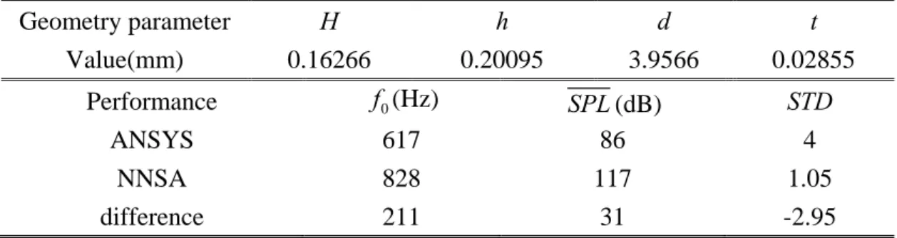
(50) utilize the geometry of diaphragm to simulate the SPL response of microspeaker by ANSYS again. Results obtained via ANSYS and NNSA are shown in Table15. It shows that the difference of performance has very high drop height as a result of too less training set of input-output pairs.. 33.

(51) 6. Conclusions FEA-lumped parameter model has been presented for electroacoustical simulation of microspeakers. The mechanical impedance obtained from the FEA model of the diaphragm-voice coil assembly is incorporated into the lumped parameter model of the microspeaker system. The integrated EMA model provides better prediction for the voice-coil impedance and the SPL response at high frequencies than the conventional lumped parameter approach that neglects the higher-order flexural modes of the diaphragm. On the basis of the proposed model, the dimensions of diaphragm are optimized with the aid of the Taguchi method. Using the results of the Taguchi method as a starting point, the optimal number of diaphragm corrugation is determined using sensitivity analysis. According to the optimized design of Table 6, the fundamental resonance frequency has been decreased and the flatness of the SPL response has been improved over the non-optimized design. In terms of the SPL frequency responses of Run 7 for different number of corrugation in Fig 18(b) reveals that SPL will increase with adding number of corrugation. FEA-lumped parameter model is also employed to the simulation of vented-box system that can predict the high frequency behavior of SPL response. Constrained optimization techniques were also employed to find the design that maximizes the sound pressure output of the vented-box system under practical constraints. Another optimization method of dimensions of diaphragm geometry is NNSA. Using the intelligent modeling of NN system which can predict the performance of SPL response, the optimal dimensions of diaphragm geometry is estimated via SA method.. According to the optimized dimensions of diaphragm geometry, the. performance of SPL response is calculated again to prove the accuracy of prediction.. 34.

(52) The high difference shown in Table 15 reveals that dimension of diaphragm geometry which is not involving in the training set of input-output pair causes the high variation of performance of SPL response. This phenomenon bringing about high difference is due to the insufficient of the training set of input-output pairs which aren’t easy to produce via ANSYS.. 35.

(53) 7. APPENDIX The measurement of loudspeaker efficiency Loudspeaker efficiency is defined as the sound power output divided by the electrical power input. Most loudspeakers are actually very inefficient transducers; about 1% of the electrical energy sent by an amplifier to a typical home loudspeaker is converted to the acoustic energy we can hear. The remainder is converted to heat, mostly in the voice coil and magnet assembly. The main reason for this is the difficulty of achieving proper impedance matching between the acoustic impedance of the drive unit and that of the air into which it is radiating.. The efficiency of. loudspeaker drivers varies with frequency as well. For instance, the output of a woofer driver decreases as the input frequency decreases.. I.. Calculate Loudspeaker Efficiency based on TS parameters The reference on-axis sensitivity of a driver is defined as the SPL at 1m away. from the loudspeaker for a voice-coil voltage 1Vrms or. RE Vrms. The latter is the. rms voltage required for a power of 1W into a resistor of value RE , i.e. the voice-coil resistance.. V W and SPL1sens , The sensitivity can be denoted as two type SPL1sens. respectively. They could be approximated by TS parameters and given by V SPL1sens (dB ) = 20 log10 (. W SPL1sens (dB ) = 20 log(. ρ0 Bl. 2π S D RE M AS. ρ 0 Bl. 2π S D RE M AS. ) + 94. ) + 94 + 20 log10 RE. (72). The TS parameters are shown in Table 16. The efficiency η of a driver is defined as follow:. η=. PAR PE. (73). where PAR is the acoustic power radiated to the front of the diaphragm and PE is 36.

(54) the electrical input power to the voice coil.. This expression is a function of. frequency. The efficiency could be estimated by TS parameters. It is given by. η=. ρ 0 B 2l 2 S D 2 ρ 0 B 2l 2 S D 2 1 2 2 ( ) G j G ( jω ) ω = 2 2 2 2π c RE M MS 2π c RE M MS Real ( 1 ). (74). Zvc. where G ( jω ) is the second-order high-pass transfer function given by. G ( jω ) =. ( s / ωs ) 2 ( s / ωs ) 2 + (1/ QTS )( s / ωs ) + 1. (75). where ωs is the resonance frequency, QTS is the total quality factor. A loudspeaker with an efficiency of 100% would output 1W energy for 1W input. At this condition it could be obtained SPL of 112.02dB. It follows the relation between sensitivity and efficiency as W SPL1sens (dB) = 112.02 + 10 log10 (η ). (76). Therefore, the efficiency can be obtained by the measured result of the 1m on-axis SPL from Eq. (76).. Fig 27 shows the efficiency comparison between. experiment and simulation.. Blue line is the result of the measured efficiency. obtained by Eq. (76). The result of efficiency simulation are red and green lines. Red line is derived by the left formula of Eq. (74). Green line is computed by the right formula of Eq. (74). And black dotted line is calculated with G ( jω ) = 1 . The calculation of miniature loudspeaker efficiency is about 0.0536% at 2k Hz. II. Calculate loudspeaker efficiency based on the measured response According to the Eq. (73), loudspeaker efficiency can also be estimated based on the sound power and the electrical power obtained by experiment. Relation between sound pressure and sound power is given by. W =. p 2 rms 2π r 2 ρ0 c. (77). Thus we can obtain the sound power via measuring the sound pressure.. 37. The.