國立交通大學
電子工程學系 電子研究所
碩 士 論 文
具有模組選擇能力之延遲最佳化
數位微流體生物晶片合成技術
Latency-Optimization Synthesis with
Module Selection for Digital Microfluidic Biochips
研 究 生:劉廣正
指導教授:黃俊達 博士
具有模組選擇能力之延遲最佳化
數位微流體生物晶片合成技術
Latency-Optimization Synthesis with
Module Selection for Digital Microfluidic Biochips
研究生:劉廣正 Student: Kuang-Cheng Liu
指導教授:黃俊達 博士 Advisor: Dr. Juinn-Dar Huang
國立交通大學
電子工程學系 電子研究所
碩士論文
A Thesis
Submitted to Department of Electronics Engineering & Institute of Electronics College of Electrical & Computer Engineering
National Chiao Tung University in Partial Fulfillment of the Requirements
for the Degree of Master of Science
in
Electronics Engineering September 2012
Hsinchu, Taiwan, Republic of China
i
具有模組選擇能力之延遲最佳化
數位微流體生物晶片合成技術
研究生:劉廣正 指導教授:黃俊達 博士
國立交通大學
電子工程學系 電子研究所碩士班
摘 要
數位微流體生物晶片是近年生醫電子領域的研發成果,可用以取代現行生化實 驗所使用的大型分析儀器,以提升實驗效率和節省實驗成本。然而,要將各式各樣 的生化反應轉移至生物晶片上進行,工程極為繁複,因此需要設計自動化工具的協 助。縮短總反應時間是生物晶片合成程序最佳化的主要目標之一。為了進一步縮短 反應時間,模組選擇的能力是不可或缺的。大多數現行具備模組選擇能力的合成方 法皆為非決定性的方法,如基因演算法或禁忌搜尋演算法。然而,此類方法耗費過 多的電腦執行時間而無法達到及時合成。本篇論文提出了一個具備模組選擇能力以 達成延遲最佳化的數位微流體生物晶片合成方法,簡稱 LOSMOS。此方法利用減 少晶片上的儲存液滴的數量、並套用以系統延遲為標的的迭代重綁定過程,有效率 地完成數位微流體晶片合成及降低總反應時間。根據實驗結果,LOSMOS 比所有 已知的合成方法更出色;包含目前最新的方法 Path-scheduler,平均而言較其減少 了 18.22%的反應時間;且甚至超越了沒有模組選擇能力的整數線性規劃求得的最 佳解─且僅需要極小的運算時間而已。ii
Latency-Optimization Synthesis with
Module Selection for Digital Microfluidic Biochips
Student: Kuang-Cheng Liu Advisor: Dr. Juinn-Dar Huang
Department of Electronics Engineering & Institute of Electronics
National Chiao Tung University
Abstract
Digital microfluidic biochip (DMFB) is a latest development in biomedical electronics. DMFBs can replace traditional bench-top equipments, which are generally costly and bulky, to accelerate processes and save the costs of biochemical experiments. However, synthesis of various reactions on a biochip is a complicated work and thus needs the help of design automation tools. One of the major optimization goals of DMFB synthesis is latency minimization. To minimize the assay latency, module selection must be considered in synthesis flow. Most of current approaches with module selection capability adopt non-deterministic methods, such as genetic algorithms or Tabu searches. These methods may consume lots of runtime and thus make online (real-time) synthesis impossible. In this thesis, I propose an efficient latency-optimization synthesis with module selection ability, named LOSMOS. It minimizes assay latency by storage minimization and latency-driven iterative rebinding. Experimental results show that LOSMOS outperforms all the previous works, including the state-of-the-art Path-scheduler by 18.22% in terms of latency reduction; and even does better than an optimal ILP-based scheduler without module selection in most cases with very little runtime.
iii
誌 謝
首先我要謝謝我的指導教授—黃俊達副教授,在碩士的兩年當中,給予充分 的時間修習研究所相關專業課程,並在每周實驗室會議上耐心的指導與建議。在 論文研究上,也樂於安排個別會議上細心的給予寶貴的意見。並且在實驗室自由 學系的風氣下,培養出獨立思考及解決問題的能力,也能學習到與其他人的團隊 合作,對老師的感恩之情,無法以簡短的文字來形容。 再來我要感謝我的父母,在我挫折的時候不斷鼓勵我讓我完成學業。也要感 謝我的師父,"妙禪"師父讓我有安定的心來完成實驗。而也謝謝在百忙之中抽空 參加口試的委員—周景揚教授、張世杰教授和林永隆教授,你們的意見讓我受益 良多,非常的感謝。 另外謝謝博士班的學長姐,尤其是帶領我作研究的劉家宏學長(宏哥),他對 研究的熱忱還有非常嚴謹的研究態度讓我體驗到作研究的樂趣。還有實驗室的同 學—許晉維(包子)、陳怡庭(馬力)、謝明廷(阿副)和賴鵬先(神),感謝你們和我一 起在碩士的生涯中一起奮鬥、努力,和你們在一起是我珍貴的回憶。最後謝謝實 驗室的學弟妹—偉豪、惠珊、建宇和子敬,在口試時幫我打理一切,感謝你們。 希望大家在未來的日子裡,都能順順利利完成自己的研究,也希望這篇論文 對生物科技的進步能有小小的貢獻,再次感謝所有幫助我的人。iv
Contents
摘 要... i Abstract ... ii 誌 謝... iii List of Tables ... v List of Figures ... vi Chapter 1 Introduction ... 1Chapter 2 Digital Microfluidic Biochip ... 4
2.1 Architecture ... 4
2.2 Fluidic Operations ... 6
2.3 Sequencing Graph Model ... 8
2.4 High Level Synthesis of DMFBs ... 9
Chapter 3 Previous Works ... 11
3.1 Without Module Selection ... 11
3.2 With Module Selection... 13
Chapter 4 Motivations ... 14
4.1 Effects of Storage Units ... 14
4.2 Module Selection Issue ... 17
Chapter 5 Proposed Algorithm ... 18
5.1 Overview ... 18
5.2 Storage Minimization Scheduling ... 20
5.3 Iterative Operation Rebinding... 24
5.3.1 Operation Rebinding ... 25
5.3.2 Latency Gains ... 27
Chapter 6 Experimental Results ... 29
Chapter 7 Conclusion ... 32
v
List of Tables
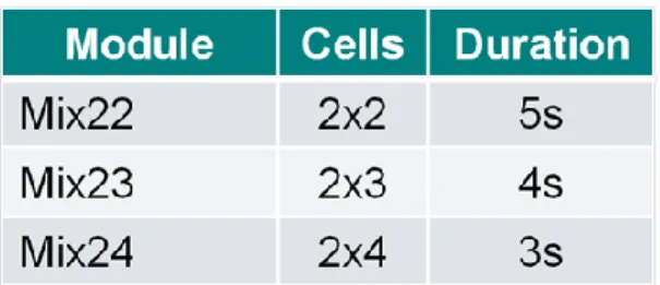
Table 1. All kinds of module for a mixing operation ... 7
Table 2. Experiment 1 multiplexed in-vitro diagnostics ... 30
Table 3. Experiment 2 sample preparations ... 31
vi
List of Figures
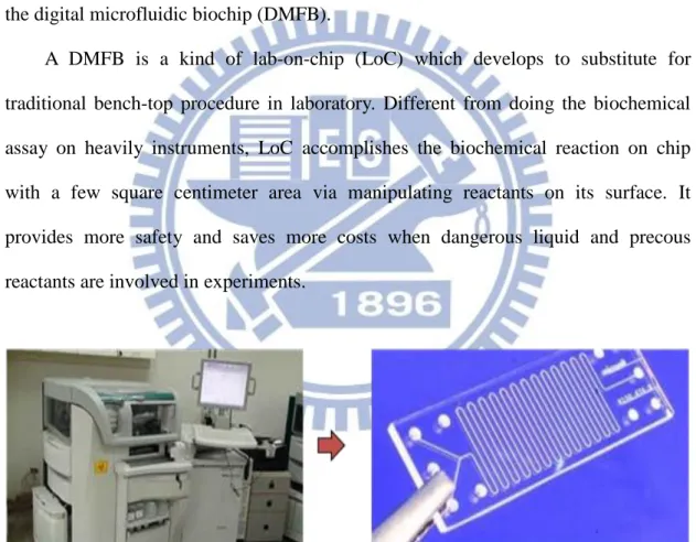
Figure 1. A LoC substitutes bench-top procedure in laboratory ... 1
Figure 2. (a) DMFB architecture ... 5
Figure 2. (b) A cell with detector...5
Figure 3. Routing patterns... 6
Figure 4. Biochemical assay ... 8
Figure 5. Sequencing graph ... 8
Figure 6. An example of operation binding ... 9
Figure 7. An example of operation scheduling ... 10
Figure 8. (a) Scheduling step in the first four cycle ... 12
Figure 8. (b) An assay and chip architecture...12
Figure 9. All paths of a sequencing graph... 12
Figure 10. An example of the inflexible scheduling rule ... 15
Figure 11. (a) A complex reaction ... 15
Figure 11. (b) PS...15
Figure 11. (c) M-LS...15
Figure 12. All possible value of storage saving factor ... 16
Figure 13. Comparison between non-module selection and module selection ... 17
Figure 14. The overview of proposed algorithm ... 18
Figure 15. An example of proposed scheduling rule ... 21
Figure 16. (a) An sequencing graph of an assay ... 22
Figure 16. (b) Scheduling result using the priority only consider critical path ... 22
Figure 17. (a) A changed scheduling order ... 23
Figure 17. (b) Scheduling result using proposed priority...23
Figure 18. Overall flow of SMS ... 23
Figure 19. Flow of iterative operation rebinding ... 24
Figure 20. (a) A graph with 3 mixing operation c, f, and g without rebinding ... 25
Figure 20. (b) All BPs of operations without rebinding...25
1
Chapter 1
Introduction
Biochip technology is one of the most critical eras in hi-tech industry nowadays. The annual report of International Technology Roadmap for Semiconductors (ITRS) points out that biochip is a solution to achieve “More than Moore”, and explores functional diversification of CMOS [1][2]. One of the emerging topics of biochip is the digital microfluidic biochip (DMFB).
A DMFB is a kind of lab-on-chip (LoC) which develops to substitute for traditional bench-top procedure in laboratory. Different from doing the biochemical assay on heavily instruments, LoC accomplishes the biochemical reaction on chip with a few square centimeter area via manipulating reactants on its surface. It provides more safety and saves more costs when dangerous liquid and precous reactants are involved in experiments.
Traditional LoCs manipulate continuous flow with micro-channels. The movement of reagents and buffers are controlled by microvalves and integrated micropumps. According to the fixed micro-channels, this type of biochip can only
2
serve for a specific biochemical assay. In contrast, the digital microfluidic biochip (DMFB) dispenses reagents as discrete droplets and manipulates them by applying different control voltages to electrodes under chip's surface [3][4]. Therefore, different reactions can be finished in the same chip architecture without any device change. DMFB provides a general solution for bioassay instead of a specific purpose. Other advantages of DMFBs are low manufacturing cost, portability, high-throughput, reconfigurable, and higher reliability since less human involved [5]. According to these features, DMFB is suitable to perform applications as clinical diagnostics, environmental toxicity monitoring, and point-of-care diagnosis [6]. Designing a DMFB to meet a variety of applications is a considerable work. Any minor change in original reaction will lead to redesign. Therefore, design automation is indispensable to reduce human cost. With the increased demands of biochips, lots of works have been proposed to deal with problems in the DMFB design flow. According to [7], DMFB design flow consists of two stages, fluidic-level synthesis and chip-level design. The first part, fluidic-level synthesis, focuses on droplet manipulating. It covers complicated problems like sample preparation [8] operation scheduling and operation binding [19], module placement [20][22], and droplet routing [23][26]. Instead of fluid control, manufacture problems are the major concerns in the second part, such as pin assignment and wiring [27][29].
the front-end of fluidic-level synthesis, named high-level synthesis, includes two parts: operation binding and operation scheduling. The two parts are the most determinant of assay latency. If the operations are scheduled and bound attentively, the assay latency can be certainly minimized. However, as far as we know, there still some problems are not well-considered in current high-level synthesis flow, such as storage unit control and module selection. High amount of storage units may occupy much area, lessen available mixing space, and then leads to long assay latency or
3
infeasible scheduling. Moreover, module selection provides more possibility to enhance utilization of array area. It leads to shorter latency. However, previous works with module selection ability are all non-deterministic algorithms which are time-consuming. Thus, a deterministic synthesis with module selection ability must benefit the DMFB design flow. This work proposes a latency-optimization synthesis with module selection, LOSMOS, to solve the operation scheduling and the operation binding problem. LOSMOS is based on list scheduling and thus is very efficiency. The experimental results show that LOSMOS obtains better results than most of previous works with less execution time. The remainder of this work is organized as follows. Chapter 2 briefly reviews the DMFB architecture and previous works. Our motivation is described in Chapter 3. In Chapter 4, we describe the problem formulation and present the proposed algorithm. In the end, we verify our algorithm by experimental results in Chapter 5 and conclude this work in Chapter 6.
4
Chapter 2
Digital Microfluidic Biochip
2.1 Architecture
A DMFB architecture is a 2-D array of cells as shown in Figure 2(a). Each cell consists of two glass plates which are coated with indium tin oxide (electrode), parylene C (insulator) and Teflon AF (hydrophobic surface). Indium tin oxide (ITO) electrodes are used to drive droplets by electrowetting-on-dielectronic (EWOD) effect. It implies the potential change leads to the surface intension change of fluids, and makes them lean to active electrodes. In general, most droplets can be transported at 20Hz with the 1.5mm pitch [3][4]. It means that a droplet can cross more than 20 electrodes within a second (0.05sec/electrode). Compared with the duration of other assay operations like mixing (6~10sec), the routing time is thus negligible. Parylene C, a dielectric insulator which is coated with Teflon AF (hydrophobic surface), is allocated on the top and bottom plates to decrease the wettability of the surface and to add capacitance between the droplet and the electrode. Furthermore, to prevent evaporation of droplet and to smooth the movement, immiscible silicon oil will be put in the space between two plates [3]. In additional to cells, there are other devices including reservoirs, dispensing ports and detecting cells in a DMFB, as shown in Figure 2(a). Reservoirs and dispensing ports usually located on the side of the DMFB. The droplet is formed from a reservoir and enters the chip through the dispensing port. For avoiding liquid contamination, one reservoir should be dedicated to one kind of reactants. The other component, detecting cell (detector), is used to evaluate the property of a droplet. The structure of a detector is decided by the assays to be
5
performed. For example, the optical detectors suit the colorimetric assay [13]. In this case, a photodiode and light-emitting diode are placed over the top and under the bottom of the cell respectively, as show in Figure 2(b).
Glass
Glass
Droplet
Indium Tin Oxide (ITO) electrodes Photodiode
LED High voltage
(a) (b) Electrodes (2D array) Droplet Reservoirs Detector Bottom glass plate array size=16(cells)
Figure 2. (a) DMFB architecture and (b) A cell with detector (a)
6
2.2 Fluidic Operations
There are three kinds of fluidic operations in a DMFB, including the dispensing operation, the detecting operation, and the mixing operation. A dispensing operation means that a dispensing port injects a droplet from a reservoir into the chip. A detecting operation means routing a droplet to a detecting cell and evaluating its property. The operations mentioned above all operate on the real device (reservoirs, dispensing ports, and detecting cells). However, mixing operation operates on a cell group which does not locate on a specific position. This cell group is composed of adjacent cells. Two droplets are combined and then moves rapidly among adjacent cells to finish mixing operation. While a mixing operation is finished, all cells used by the mixing operation will be freed immediately. Those cells can be used by the other operation again. According to this property, a mixing operation is also called a reconfigurable operation. Besides, the group of adjacent cells which can perform mixing operation is also called a “module”. The performance of a module is related by its size and routing pattern. Figure 3 shows possible routing patterns. Since the module with large size has longer straight path to accelerate a droplet, it leads to shorter duration. Table 1shows different module types.
7
8
2.3 Sequencing Graph Model
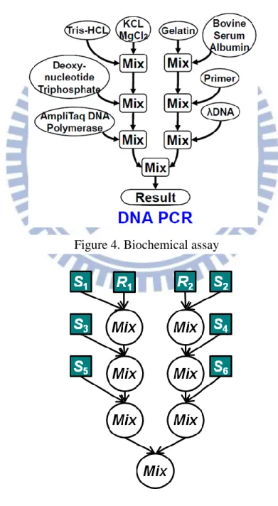
A biochemical assay, as shown in Figure 4, can be formulated as a set of fluidic operations. The relation between fluidic operations can be represented by sequencing graph model, as shown in Figure 5. In the sequencing graph model, each node indicates a fluidic operation and the edge between two nodes means their dependence and the droplet routing between two operations.
Figure 4. Biochemical assay
9
2.4 High Level Synthesis of DMFBs
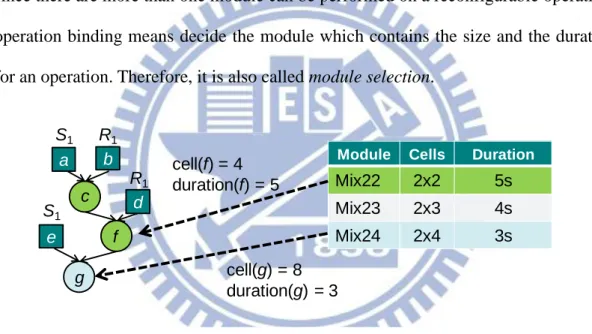
High-level synthesis (HLS) plays an important role in the front end of biochip synthesis. It always contains two parts: operation binding and operation scheduling. These procedures are crucial for determining the latency of an assay. For operations performing on real devices like the dispensing port and the detector, operation binding indicates that to assign a real device to perform an operation. Each device can only execute one operation at a time. On the other hand, for the reconfigurable operations, since there are more than one module can be performed on a reconfigurable operation, operation binding means decide the module which contains the size and the duration for an operation. Therefore, it is also called module selection.
After operation binding, the size and the duration of all operations are known. Operation scheduling can be performed after. Operation scheduling decides the start and the end cycle of all operations without dependency and resource violation to minimize the total latency. Since a sequencing graph is similar to a data flow graph in VLSI synthesis, we can refer to the algorithms used in VLSI design (e.g., list scheduling) to solve scheduling problem. However, different from the VLSI scheduling, storage units play an important role in DMFBs. A storage unit is happened
Module Cells Duration
Mix22 2x2 5s Mix23 2x3 4s Mix24 2x4 3s cell(f) = 4 duration(f) = 5 cell(g) = 8 duration(g) = 3 c f g e a b d S1 R1 S1 R1
10
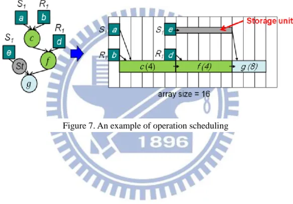
when two dependent operations are not scheduled closely. 1-cell space is needed to keep the resultant droplet of the former operation. The storage unit is not vanished until the next operation uses it. Taking Figure 7 for example, a storage unit needs to store the resultant of operation e since operation g cannot be scheduled right after operation e. Because storage units may also use the area which mixing operations need, controlling the amount of storage units is necessary to achieve an efficient scheduling result.
11
Chapter 3
Previous Works
3.1 Without Module Selection
The approach [10] is the first work mentioned scheduling problem as far as we know. It formulated the biochip scheduling problem and proposed an ILP algorithm to solve this problem. In the ILP algorithm, all operations bind to the fastest module for simplify the complexity and a PCR reaction example are introduced. [11] is a successor of [10]. In [11], the ILP model has been further refined. The area constraint issue and more operation types like detecting operation are considered. This method can guarantee an optimal solution. Since the ILP method is hard to deal with larger cases, two heuristics, the heuristic based on a genetic algorithm (GA) and the modified list scheduling algorithm (M-LS), were proposed in [11]. The former one GA is based on list scheduling and the priority of operations is decided by genetic algorithm. However, GA may also suffer from long execution time. Therefore, a hybrid genetic algorithm (HGA) was developed to shorter the execution time of GA through searching space reduction [12]. However, HGA is a special purpose algorithm for in-vitro cases. The latter one M-LS, schedules operations in the increasing order of their criticality, i.e., the longest path from an operation to the sink. M-LS is very efficient and can be finished in very short time. However, it suffers from the storage excess problem. Although M-LS uses the rescheduling step to solve this problem, it may still be stuck in high fan-out graph. Figure 8(a) shows a rescheduling step example by scheduling the assay in Figure 8(b) on a biochip which contains a 2-D array with 16 cells and four ports, S1, R1, S2, and R2. At cycle three, since operation e
12
and operation j could not be scheduled, storage units are needed to store the resultants of operation d and operation i. However, the used area is out of total area. The rescheduling step must be performed. The step is achieved by going back to the previous step. Then, reschedule the latest scheduled operation until the used area fits the area constraint.
Path-scheduler (PS) avoids excess storage problem by scheduling a whole path, like the nodes with same color in Figure 9, instead of individual operations [17], and performs better than M-LS in high fan-out graph with different priority setup. There also has an optimal scheduler [18] which can deal with the storage excess problem, but it only suits the assay that can be formulated as a full binary tree.
a b f g 1 2 3 4 a b f g c (8) h (8) 1 2 3 4 d a b f g c (8) h (8) 1 2 3 4 d a b f g c (8) 1 2 3 4 d i i i (a) (b) cycle = 1 cycle = 2 cycle = 3 cycle = 4
Figure 8. (a) Scheduling step in the first four cycle (b) An assay and chip architecture
Figure 9. All paths of a sequencing graph
a
b
c
13
3.2 With Module Selection
The methods mentioned above do not consider the module selection and the performance is thus limited. The extended GA [14] and the Tabu-search based algorithm (Tabu) [15] are existing algorithms which consider the module selection. The extended GA inherits from [10] and adds binding information into the chromosome to achieve module selection. The latter method Tabu starts with a solution in which operations are bound to modules at random. It then use Tabu searching to find the best binding result and use list scheduling to schedule operations. Even if these two methods, the extended GA and the Tabu, permit module selection. However, they are all stochastic optimization method and are difficult to apply in online scheduling. As a result, a fast algorithm equipped with module selection ability is indispensable.
14
Chapter 4
Motivations
4.1 Effects of Storage Units
A storage unit exists if two dependent operations are not sequentially scheduled. Since the storage units occupy chip area, the number of storage units located on a chip is inversely proportional to the amount of mixing space. Therefore, how to minimize the storage units is a crucial issue for latency minimization. For elaborating the effect of storage units, we further classify a storage unit as a dispensing storage unit (std) or
an intermediate storage unit (stm) in this work. The first one, std, appears between a
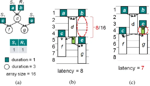
dispensing operation and a reconfigurable operation. Previous works [12], [15], and [18] schedule the dispensing operation and the reconfigurable operation sequentially to ensure no std. However, this inflexible scheduling rule may lead to the worse
latency. Take Figure 10 as an example. At first, we will schedule the assay like Figure 10(a) by the list scheduling and the scheduling rule mentioned above on a biochip consists of a 2-D array with 16 cells and two ports, S1 and R1. The scheduling result is
shown in Figure 10(b). As we can see in Figure 10(c), if we schedule operation e earlier and permit one cycle delay between operation e and operation g, the latency can be reduced from 8 to 7. Accordingly, a more flexibility scheduling rule may be required.
15
The other one, stm, is a more difficult problem than std in scheduling. Path-scheduler
tries to reduce stm by scheduling an entire path, a sequence of dependent operations,
instead of operations and thus has shorter latency than M-LS in high fan-out cases (e.g., protein assay). However, with high fan-in cases or even more complex reactions, it may lead to worse efficient. Figure 11. (a)Figure 11(a) shows a complex reaction. As shown in Figure 11(b) and Figure 11(c), the result which is produced by Path-scheduler has more stm and has longer latency than the result which is produced
by M-LS.
(a) (b) (b)
(a) (c)
Figure 10. An example of the inflexible scheduling rule
Figure 11. (a) A complex reaction (b) PS and (c) M-LS
16
Therefore, we try to minimize stm in the other way. We observed that the number
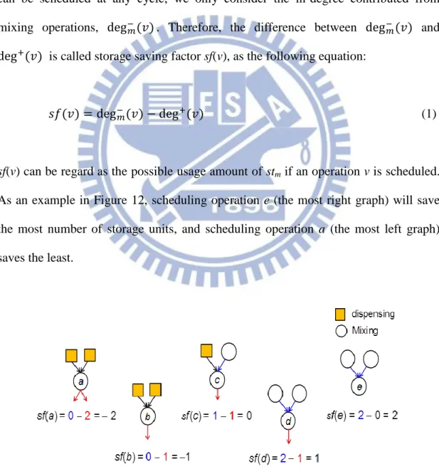
of storage units is highly related with operations’ in-/out-degree. In fact, the in-degree of an operation v, which is denoted as , implies how many droplets it required, and the out-degree of v, , means the number of resultant it produces. As a result, to schedule a vertex with high in-degree may help to minimize storage units; on the other hand, to schedule a vertex with high out-degree implies that more storage units may be produced, and vice versa. However, since dispensing operations can be scheduled at any cycle, we only consider the in-degree contributed from mixing operations, . Therefore, the difference between and is called storage saving factor sf(v), as the following equation:
(1)
sf(v) can be regard as the possible usage amount of stm if an operation v is scheduled.
As an example in Figure 12, scheduling operation e (the most right graph) will save the most number of storage units, and scheduling operation a (the most left graph) saves the least.
17
4.2 Module Selection Issue
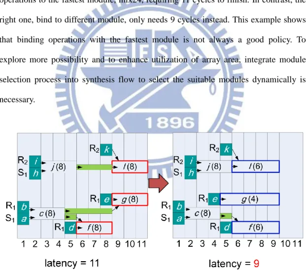
Most of previous works bind operations with the fastest (usually also the largest) module in synthesis. It helps to simplify the problem and is useful if the array size is large enough. However, in most cases, especially as segregation area is wrapped around, this strategy may be ineffective, and modules with large size may make the array overcrowded. For example, five mixing operations are scheduled with two different binding in Figure 13 using the modules in Table 1. The left one, bind all operations to the fastest module, mix24, requiring 11 cycles to finish. In contrast, the right one, bind to different module, only needs 9 cycles instead. This example shows that binding operations with the fastest module is not always a good policy. To explore more possibility and to enhance utilization of array area, integrate module selection process into synthesis flow to select the suitable modules dynamically is necessary.
18
Chapter 5
Proposed Algorithm
5.1 Overview
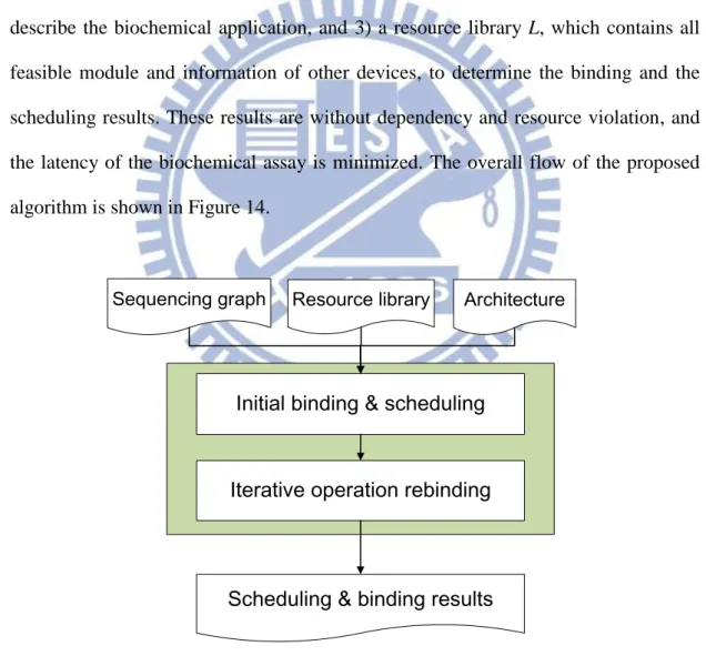
The problem formulation of this work is as following: given three information, 1) DMFB architecture, which consists of chip size, the count of dispensing ports, number of detecting cells or other functional devices, 2) a sequencing graph G, which describe the biochemical application, and 3) a resource library L, which contains all feasible module and information of other devices, to determine the binding and the scheduling results. These results are without dependency and resource violation, and the latency of the biochemical assay is minimized. The overall flow of the proposed algorithm is shown in Figure 14.
Sequencing graph Resource library
Initial binding & scheduling
Iterative operation rebinding
Scheduling & binding results
Architecture
19
In the beginning of the process, bind all operations to the fastest module (all the operations are bound). Then, a scheduler, storage minimization scheduling, based on list scheduling is performed to obtain an initial scheduling result. Following, the initial solution will be sent to the iterative operation rebinding process to refine the solution iteratively. More details of the storage minimization scheduling and iteratively operation rebinding processes will be described in section 5.2 and section 5.3.
20
5.2 Storage Minimization Scheduling
Storage minimization scheduling (SMS) is derived from the well-known list scheduling algorithm. At first, all ready operations are put in the ready list (Lready).
There are four kinds of ready operations as following: 1) a dispensing operation, 2) a mixing operation whose parents are dispensing operation, 3) a mixing operation whose parents are a dispensing operation and a finished mixing operation and 4) a mixing operation whose parents are two finished mixing operation. Then, schedule operations in ready list (Lready) one by one in each cycle according to their priority.
Compared to conventional list-based scheduling in DMFB, we schedule dispensing operations more flexible and propose a new priority. Previous works, like [12], [15] and [18], discard dispensing operations from the ready list, Lready, since these
operations can be scheduled at any cycle if there are enough resource ports. The dispensing operations and their successor operations are scheduled sequentially to avoid std. This scheduling rule guarantees no std. However, it may lead long latency
due to inflexibility in scheduling dispensing operations, as describe in section 4.2. We modified the rule by scheduling dispensing operations before their successors but not necessary right before them. Figure 15 is an example of the scheduling rule. If an operation v can be scheduled at cycle t (t=3), check previous cycles from t-1 to 1 whether there are available reservoirs and enough area to save the resultant of reservoirs. The process starts form t-1, since we want to reduce the usage of std as
more as possible. If there are available reservoirs at cycle 1 and enough area to save resultant at cycle 2, schedule dispensing operations of operation v at cycle 1. Otherwise, schedule the other operation.
21
In section 4.1, we realize that PS has a bad result with the complex graph since it entirely minimizes stm but ignores the critical path issue. Therefore, we proposed a
priority as following:
(2)
The proposed priority considers the critical path and stm minimization at the same
time. Since sf(v) implies the reduction of stm, we use it to indicate stm minimization.
However, since sf(v) is quite smaller than each path length, we multiply sf(v) and a constant to balance its value. This constant is a significant large number which is usually set a half of the critical path length. An example in Figure 16(a) will be demonstrated to show the importance of stm minimization. At first, all mixing
operations which are presented by circular shape are bound to the fastest module whose area is 8 cells and duration is 2. According to the priority which only considers the critical path (e.g., priority of operation m = 4 and operation r = 2), assign the scheduling order to each mixing operation like the red number in both Figure 16(a) and Figure 16(b).
Exist
Schedule the other operation
22
Figure 16. (a) An sequencing graph of an assay
(b) Scheduling result using the priority only consider critical path
If operations with the same priority, set their scheduling order randomly. The scheduling result of the assay is shown in Figure 16(b) and the latency is 15. As we can see, this priority will lead to a BFS scheduling order and lots of stm. On the other
hand, if we schedule the assay in Figure 16(a) using the proposed priority, the scheduling order will changed to the red numbers in Figure 17(a). At first, operation m and operation n will be scheduled first like using the priority which only consider critical path. However, the scheduler using the proposed priority will select the operation which can save more storage units like operation r and operation s next. As a result, the proposed priority will lead a DFS scheduling result as shown in Figure 17(b) and potentially reduce the amount of stm. Therefore, the latency reduces from 15
to 13 when schedule operations using the proposed priority. Figure 18 shows the overall flow of SMS.
23
Figure 17. (a) A changed scheduling order (b) Scheduling result using proposed priority
24
5.3 Iterative Operation Rebinding
As mentioned above, the scheduling algorithm for SMS potentially minimizes the latency by reducing the amount of storage units. However, further improvement may still be achieved by rebinding which explores more possibility and to enhance utilization of array area as mentioned in section 4.2. The overall algorithm of iterative operation rebinding is depicted in Figure 19. At first, operation rebinding is performed to determine the new binding of all operations for latency minimization. If the latency for the new binding result is shorter than the previous one, the counter k is reset to M; if not, set k=k1. The process does not terminate until the counter k equals to zero.
25
5.3.1 Operation Rebinding
The objective in operation rebinding is to find the new binding result to reduce latency. The simplest way to achieve the objective is listing all possible binding results and selecting the one with the most latency improvement. However, it is not realistic. Since there are too many binding results to be checked, it will cost too much execution time. Our strategy is rebinding an operation once at a time until all operations are rebound. Here, a rebinding process in an iteration means changing the module of an operation v to another module m. (v, m) is called binding pair (BP). Take Figure 20 (a) for example. There are 3 unlocked mixing operation c, f, and g and each mixing operation can be bound to 3 possible modules according to Table 1. Due to the above conditions, there are 9 feasible BPs can be selected to rebind as shown in Figure 20(b). Therefore, operation rebinding can be regard as finding the BP with the highest latency improvement in each iteration.
(a) (b)
Figure 20. (a) A graph with 3 mixing operation c, f, and g without rebinding (b) All BPs of operations without rebinding
26
Figure 21 shows the operation rebinding flow. The first step in the flow is gain calculation. It calculates latency gains for all possible BPs with unlocked operations (i.e., operations are not rebound) to judge the latency improvement of each BP. There are two latency gains: the primary latency gain (Gp) and the secondary latency gain
(Gs). They represent the latency improvement. The physical meaning of them will be
described in section 5.3.2. After gain calculation, BP selection will be performed. The BP with the highest Gp will be selected first. Since the unchanging binding is also a
kind of rebinding processes (i.e. existing a BP with zero Gp), a BP with negative Gp
will not be considered here. If there is more than one BP with the highest Gp, the BP
with the highest Gs is selected. According to the selected BP (v, m), operation v will
be rebound to module m, and m will be locked after. Finally, rescheduling is performed by SMS to get the current latency. These steps mentioned above does not terminate until all operations are locked.
Gain calculation
Rescheduling BP selection
All operations are locked All unlocked operations
Rebind & Lock
False True
27
5.3.2 Latency Gains
There are two latency gains, primary latency gain (Gp) and secondary latency
gain (Gs) to determine the latency improvement of each BP. The first one Gp can be
represented as the following equation:
(3)
In (3), T is the latency before rebinding, and T' means the latency while the operation
v bound with the module m, and SMS is performed. The second one Gs is presented
by the following equations:
(4)
Equation (4) is composed of two parts, local latency improvement and storage unit reduction. Since Gp only represents the improvement of the critical path, some BPs
with the potential to make a shorter latency in the next iteration may be ignored. Therefore, Gs indicates this potential by the sum of end cycle improvements, ti ti', for
all operations. However, since operations locate on different paths, the importance of each end cycle improvement is not the same. To indicate differences of them, the weight in (5)(6) multiplies each end cycle improvement together.
(5)
28
(5) means the ratio between the longest path passes through an operation and the critical path length. Due to the fact that the number of storage units affects the total latency, storage unit reduction, nst nst', should also be considered. nst means the
average storage units count in each cycle before rebinding, as shown in (7). nst'
implies the average storage units in each cycle when operation v is bound to module
m. Besides, we consider that storage unit reduction is contributed by all operations.
Therefore, the number of operations, N, multiplies the storage unit reduction together.
(7)
29
Chapter 6
Experimental Results
The proposed algorithm has been implemented in C++ on a Linux machine. All experiments are conducted on workstation with an Intel Xeon 2.4GHz CPU with 72GB RAM. The ILP solver we used is Gurobi optimizer 5.0 [29]. Three real-life test cases: multiplexed in-vitro diagnostics, PCR, and Protein assay [13] and six random cases of sample preparation are used here to evaluate our algorithm. Since previous works are implemented with different area constraints and resource libraries, the experimental result they proposed can't compare with each other. Therefore, we want to re-implement them to compare with LOSMOS. Besides, the other two versions of M-LS, M-LS (DEC) and M-LS (INC) are also implemented. They are proposed in [18] to compare with PS. Both of them force dispensing operation scheduling right before their successor, but M-LS (DEC) uses the increasing order of priority and M-LS (INC) uses the inversed one. However, we cannot re-implement GA and HGA entirely and these two works only report the experimental results using multiplexed in-vitro diagnostics. LOSMOS will compare with the methods mentioned above using multiplexed in-vitro diagnostics with in-vitro resource library [13] in the first experiment. Table 2 shows the experimental result of the first experiment. Since the execution time of all methods is less than 5 sec, we do not report the table of execution time. As we can see, LOSMOS is 1.07 times faster than previous works on average. However, the improvement in LOSMOS is quite small. The reason we thought is that the number of operations in above cases are too small (16~64 operations) thus those solutions are all near optimal. Therefore, we will use cases with larger number of operations to perform in the second experiment. Due to lack of cases
30
and related resource library, we randomly generate six cases of the multiple-targets sample preparation reaction flow and use the in-vitro resource library. However, there are many set of modules and detectors can be performed. For fairly, we choose the set of module and the detector with the longest latency. The results of the second experiment are shown in Table 3. In this experiment, we find that SMS is 1.21 times faster than most previous works on average except ILP. It shows that scheduling method considering storage minimization has a lot of benefits for latency minimization. In additional to SMS, we further minimize latency using module selection ability in LOSMOS. As the last column in Table 3, LOSMOS performs 1.35 times faster on average than previous works and even 1.04 times faster than ILP with no module selection ability in short execution time (2~6 sec). Therefore, these results prove that LOSMOS can achieve good performance in large cases with little run time. Finally, we use two real cases: Protein and PCR. To evaluate our synthesis algorithm can apply in real-life in the third experiment. The resource library using here is proposed in [30]. Table 4 shows this experimental result. Since PCR only has seven operations, each algorithm achieves optimal solution. In contrast, protein is a large case. The latency of LOSMOS is equal or better than previous works.
Table 2. Experiment 1 multiplexed in-vitro diagnostics
Area (cells) Latency (cycle) ILP GA HGA M-LS M-LS (DEC) M-LS (INC) PS SMS LOSMOS In-vitro1_16 24 15 15 16 17 17 16 16 17 16 In-vitro2_24 32 17 17 18 19 18 20 19 18 17 In-vitro3_36 40 23 25 23 26 25 25 25 25 23 In-vitro4_48 56 23 26 23 27 25 26 26 25 23 In-vitro5_64 72 29 34 29 35 32 32 32 32 29 Avg. 0.98 1.07 1.01 1.14 1.08 1.10 1.09 1.08 1
31
Table 3. Experiment 2 sample preparations
Table 4. Experiment 3 two real cases: PCR and Protein
Area (cells) Latency (cycle) ILP M-LS (DEC) M-LS (INC) PS SMS LOSMOS Sample_preparation_61 100 169* 306 281 241 247 165 Sample_preparation_65 100 131 219 157 147 145 129 Sample_preparation_67 100 133 221 205 161 155 133 Sample_preparation_70 100 139* 191 177 179 153 129 Sample_preparation_78 100 -* 370 295 263 233 195 Sample_preparation_84 100 175* 291 223 - 203 163 Avg. 1.04 1.73 1.45 1.31 1.24 1
“-” The method fails in that case
“*” ILP does not terminate in 24-hours; the current best result is reported
Area (cells) Elapsed time ILP M-LS (DEC) M-LS (INC) PS SMS LOSMOS Sample_preparation_61 100 >24hr <1s <1s <1s <1s 3.2s Sample_preparation_65 100 0.7hr <1s <1s <1s <1s 2.9s Sample_preparation_67 100 3.1hr <1s <1s <1s <1s 3.1s Sample_preparation_70 100 >24hr <1s <1s <1s <1s 3.3s Sample_preparation_78 100 >24hr <1s <1s <1s <1s 6.1s Sample_preparation_84 100 >24hr <1s <1s <1s <1s 5.4s Area (cells) Latency (cycle) ILP M-LS (DEC) M-LS (INC) PS SMS LOSMOS PCR_7 100 8 8 8 8 8 8 Protein_103 100 179 267 179 215 185 179 Area (cells) Elapsed time ILP M-LS (DEC) M-LS (INC) PS SMS LOSMOS PCR_7 100 <1s <1s <1s <1s <1s <1s Protein_103 100 4.3hr <1s <1s <1s <1s 10.07s
32
Chapter 7
Conclusion
In this thesis, we proposed the latency-optimization synthesis with module selection (LOSMOS) on DMFBs. LOSMOS consists of two major parts: the storage minimization scheduling (SMS) and the iterative rebinding procedure. Because the storage count is highly related to the assay latency, the first part, SMS, takes the saving factor into consideration for storage minimization and achieves better results accordingly. The second part further iteratively evaluates and improves the binding of each operation with latency gains. According to the ability of module selection, LOSMOS outperforms a state-of-the-art method, Path-scheduler, by 18.22% in terms of latency reduction on average, and even performs better than the optimal ILP method without module selection. Undoubtedly, the good performance and short computation time make LOSMOS a promising option in DMFB synthesis.
33
References
[1] International Technology Roadmap for Semiconductors. Semiconductor Industry Association, 2011
[2] T.-Y. Ho, J. Zeng, and K. Chakrabarty, “Digital microfluidic biochip: a vision for functional diversity and more than Moore,” in Proc. IEEE/ACM International
Conference on Computer-Aided Design, 2010, pp. 578-585
[3] M. G. Pollack, A. D. Shenderov and R. B. Fair, “Electrowetting-based actuation of droplets for integrated microfluidics,” Lab. Chip, vol. 2, no.2, pp. 96-101, Feb. 2002
[4] V. Srinivasan, V. K. Pamula, M. G. Pollack, and R. B Fair, “Clinical diagnostics on human whole blood, plama, serum, urine, saliva, sweat, and tears on a digital microfluidic platform,” in Proc. Micro Total Analysis Systems, 2003, pp.
1287-1290
[5] K. Chakrabarty, “Design automation and test solutions for digital microfluidic biochips,” IEEE Transactions on Circuits and Systems I, vol. 57, no. 1, pp. 4–17, Jan. 2010.
[6] R. Sista, Z. Hua, P. Thwar, A. Sudarsan, V. Srinivasan, A. Eckhardt, M. Pollack, and V. Pamula, “Development of a digital microfluidic platform for point of care testing,” Lab. Chip, vol. 8, no. 12, pp. 2091–2104, Dec. 2008.
[7] T.-Y. Ho, K. Chakrabarty, and P. Pop, “Digital microfluidic biochips: recent research and emerging challenges,” in Proc. IEEE/ACM/IFIP Hardware/Software Codesign and System Synthesis, 2011, pp. 335–343.
[8] S. Roy, B. B. Bhattacharya, and K. Chakrabarty, “Optimization of dilution and mixing of biochemical samples using digital microfluidic biochips,” IEEE
Transactions on Computer-Aided Design , vol. 29, no. 11, pp. 1696–1708, Nov.
2010.
[9] Y.-L. Hsieh, T.-Y. Ho, and K. Chakrabarty, “On-chip biochemical sample preparation using digital microfluidics,” in Proc. IEEE Biomedical Circuits and
Systems Conference, 2011, pp. 297–300.
[10] J. Ding, K. Chakrabarty, and R. B. Fair, “Scheduling of microfluidic operations for reconfigurable two-dimensional electrowetting arrays,” IEEE Transactions
on Computer-Aided Design, vol. 20, no. 12, pp. 1463–1468, Dec. 2001.
[11] F. Su and K. Chakrabarty, “Architectural-level synthesis of digital microfluidics-based biochips,” in Proc. IEEE/ACM International Conference on
34
[12] A. J. Ricketts, K. Irick, N. Vijaykrishnan, M. J. Irwin, “Priority scheduling in digital microfluidics-based biochips,” in Proc. IEEE/ACM Design, Automation
& Test in Europe, 2006, pp. 329–334.
[13] F. Su and K. Chakrabarty, “High-level synthesis of digital microfluidic biochips,”
ACM Journal on Emerging Technologies in Computing Systems, vol. 3, no. 4, pp.
16:1–16:32, Jan. 2008.
[14] F. Su and K. Chakrabarty, “Unified high-level synthesis and module placement for defect-tolerant microfluidic biochips,” in Proc. IEEE/ACM Design
Automation Conference, 2005, pp. 825–830.
[15] E. Maftei, P. Pop, and J. Madsen, “Tabu search-based synthesis of dynamically reconfigurable digital microfluidic biochips.” in Proc. Compilers Architecture
and Synthesis for Embedded Systems, 2009, pp. 195–203.
[16] M. Alistar, E. Maftei, P. Pop, and J. Madsen, “Synthesis of biochemical applications on digital microfluidic biochips with operation variability,” in Proc.
Design, Test, Integration and Packaging conferences Symp., 2010, pp. 350–357.
[17] D. Grissom and P. Brisk, “Path scheduling on digital microfluidic biochips,” in
Proc. IEEE/ACM Design Automation Conference, 2012, pp. 26–35.
[18] L. Luo and S. Akella, “Optimal scheduling of biochemical analyses on digital microfluidic systems,” IEEE Transactions on Automation Science and
Engineering, vol. 8, no. 1, pp. 216–227, Jan. 2011.
[19] F. Su and K. Chakrabarty, “Module placement for fault-tolerant microfluidics-based biochips,” ACM Transactions on Design Automation of
Electronic Systems, vol. 11, no. 3, pp. 682–710, Jul. 2006.
[20] P.-H. Yuh, C.-L. Yang, and Y.-W. Chang, “Placement of defect-tolerant digital microfluidic biochips using the T-tree formulation”, ACM Journal on Emerging
Technologies in Computing Systems, vol. 3, no. 3, pp. 13:1–13:32, Nov. 2007.
[21] Z. Xiao and E. F. Y. Young, “Placement and routing for cross-referencing digital microfluidic biochips,” IEEE Transactions on Computer-Aided Design of
Integrated Circuits and Systems, vol. 30, no. 7, pp. 1000–1010, Jul. 2011.
[22] F. Su, W. Hwang, and K. Chakrabarty, “Droplet routing in the synthesis of digital microfluidic biochips,” in Proc. IEEE/ACM Design, Automation & Test in
Europe, 2006, pp. 323–328.
[23] M. Cho and D. Z. Pan, “A high-performance droplet routing algorithm for digital microfluidic biochips,” IEEE Transactions on Computer-Aided Design of
35
[24] P.-H. Yuh, C.-L. Yang, and Y.-W. Chang, “BioRoute: A network flow based routing algorithm for the synthesis of digital microfluidic biochips,” IEEE
Transactions on Computer-Aided Design of Integrated Circuits and Systems, vol.
27, no. 11, pp. 1928–1941, Nov. 2008.
[25] T.-W. Huang, C.-H. Lin, and T.-Y. Ho, “A contamination aware droplet routing algorithm for the synthesis of digital microfluidic biochips,” IEEE Transactions
on Computer-Aided Design of Integrated Circuits and Systems, vol. 29, no. 11,
pp. 1682–1695, Nov. 2010.
[26] C. C.-Y. Lin and Y.-W. Chang, “ILP-based pin-count aware design methodology for microfluidic biochips,” IEEE Transactions on Computer-Aided Design of
Integrated Circuits and Systems, vol. 29, no. 9, pp. 1315–1327, Sep. 2010.
[27] T. Xu, K. Chakrabarty, and V. K. Pamula, “Defect-tolerant design and optimization of a digital microfluidic biochip for protein crystallization,” IEEE
Transactions on Computer-Aided Design of Integrated Circuits and Systems, vol.
29, no. 4, pp. 552–565, Apr. 2010.
[28] Y. Zhao, K. Chakrabarty, R. Sturmer, and V. K. Pamula, “Optimization Techniques for the Synchronization of Concurrent Fluidic Operations in Pin-Constrained Digital Microfluidic Biochips,” IEEE Transactions on Very
Large Scale Integration Systems, vol. 20, no. 6, pp.1132–1145, Jun. 2012.
[29] Gurobi. [Online]. Available: http://www.gurobi.com/
[30] Benchmarks for Digital Microfluidic Biochip Design and Synthesis. Available: