大型網路狀態取決路由：提升最短路徑路由的個案研究

全文

(1)國立交通大學電信工程學系碩士班碩士論文. 大型網路狀態取決路由: 提升最短路徑路由的個案研究 A Scalable State-Dependent Routing: A Case Study for Boosting Shortest Path Routing. 研究生︰陳憲良指導教授：廖維國博士. 中華民國九十四年十月.

(2) 大型網路狀態取決路由：提升最短路徑路由的個案研究. A Scalable State-Dependent Routing: A Case Study for Boosting Shortest-Path Routing 研究生︰陳憲良指導教授︰廖維國博士. Student: Sian-Liang Chen Advisor: Dr. Wei-Kuo Liao. 國立交通大學電信工程學系碩士論文. A Thesis Submitted to the Department of Communication Engineering College of Electrical Engineering and Computer Science National Chiao Tung University in Partial Fulfillment of the Requirements for the Degree of Master of Science In Communication Engineering Oct 2005 Hsinchu, Taiwan, Republic of China 中華民國九十四年十月 ii.

(3) 大型網路狀態取決路由：提升最短路徑路由的個案研究研究生︰陳憲良. 指導教授︰廖維國博士. 國立交通大學電信工程學系碩士班. 中文摘要在普通網路上，我們關注於使用馬可夫決策過程(Markov Decision Process)和最大流量演算法，來找到一種路由的方式作為提升原本的最短路徑路由的效能，並且同時提供在大型網路上的可行性。本篇論文中，我們研究並列舉了不同觀念下的其他路由方法。我們的方法則是將系統模擬成可意識到資源需求的馬可夫決策過程，並將路由資訊粗化的觀念同時加入於其中。因此依據最近一個粗化過的路由訊息，這個方法能夠決定每個服務連結該走的路徑。接著模擬網路時，是針對不同的波松分布的，找一個特殊的網路來作例子。最後與最短路徑路由比較，我們的方法能夠達到減低網路上流量阻塞的機率，並且減低了在作路由時的過度通訊花費。. iii.

(4) A Scalable State-Dependent Routing: A Case Study for Boosting Shortest-Path Routing English Abstract. Student: Sian-Liang Chen. Advisor: Dr. Wei-Kuo Liao. Department of Communication Engineering National Chiao Tung Universit. Abstract. We have an interest in using Markov decision theory and Maxflow algorithm to find a policy for boosting shortest-path routing and providing network scalability. In this thesis, we study and list other routing strategies with different concepts. Our problem is modeled as a Markov decision process with an awareness of resource requirements and a certain extent of aggregation is added at the same time. This policy determines the route of each connection based on the latest aggregated information. A case study of a network is simulated with different Possion traffic rates according above assumptions. Finally we arrive at the goal of reducing the blocking probability of the network and the communication overhead can also be endured.. iv.

(5) 誌謝在此首先感謝我的指導教授廖維國老師，在碩士班兩年的時間中，對於我的研究方法、原則以及日常生活的態度，不厭其煩地給予諄諄教誨，使得我在短短兩年之間能夠學會面對研究、課業，甚至於生活該有的態度及想法，讓我著實獲益良多。其次感謝此次擔任我口試時的兩位委員，李程輝老師和蔡明哲老師，提供了不少研究方面的寶貴意見。接著感謝我的父母，在金錢以及精神上的全力支持，使我在面對難題時，更能鼓起勇氣，全心全意地繼續作下去，達成我的理想與目標。另外論文的完成，還要感謝實驗室的學長們，有你們的經驗傳承，使我能夠避免掉研究過程中的種種困境，讓我在過程裡走的更平坦；還有實驗室裡的各位同學及可愛的學弟妹，健智、于彰、賢宗、柔嫚、廷任、佳甫、裕翔、為凡、俊宏、富元、永裕，你們的一路相陪，讓我在研究的道路上感到絲絲的溫馨，有你們在，實驗室充滿了歡笑，是我過了許久仍回味無窮的珍貴回憶。最後還要感謝我的大學同期以及身邊週遭的各位朋友，在我作研究之餘，給于我相當多生活的歡笑以及鼓勵，也是有了你們，才使得我能夠一路劈荊斬棘，謝謝你們對我的支持鼓勵。. v.

(6) Contents Chinese Abstract ....................................................................................................................... iii English Abstract ........................................................................................................................ iv Acknowledgment........................................................................................................................ v Contents ..................................................................................................................................... vi List of Tables............................................................................................................................... 1 List of Figures............................................................................................................................. 1 Introduction................................................................................................................................ 2 Survery Study of Routing Strategies ........................................................................................ 4 2.1 Strengths and Weaknesses of Shortest-Path Routing..................................................... 7 2.2 Strengths and Weaknesses of Markov Decision Algorithms for Dynamic Routing ...... 8 2.3 Strengths and Weaknesses of State-Dependent Routing with Trunk Reservations ....... 9 2.4 Strengths and Weaknesses of Call Admission and Routing in Multi-service Loss Networks .............................................................................................................................. 9 2.5 Strengths and Weaknesses of QoS Routing for Integrated Services Networks ............. 9 2.6 Strengths and Weaknesses of Hierarchical Source Routing using Implied Costs ....... 10 Background Knowledge ...........................................................................................................11 3.1 Continuous-time Markov Decision Process .................................................................11 3.2 Largrangian Multipliers ............................................................................................... 17 3.3 Maximum Flow Algorithm .......................................................................................... 18 Proposed Scheme ..................................................................................................................... 24 4.1 Link State Aggregation ................................................................................................ 24 4.2 Node Maxflow Source Routing Algorithm.................................................................. 27 Numerical Results .................................................................................................................... 29 Conclusion ................................................................................................................................ 39 Reference .................................................................................................................................. 40. vi.

(7) List of Tables Table 5.1 Types of congestion level.……………………….…………………………36 Table 5.2 Blocking probabilities of shortest path routing under various arrival rates.………………………………………………….……………………39 Table 5.3 Blocking probabilities of Maxflow source routing using Case I under various arrival rates.…..………………...…………………………………40 Table 5.4 Blocking probabilities of Maxflow source routing using Case II under various arrival rates………………………..………………………………41 Table 5.5 Blocking probabilities of Maxflow source routing using Case III under various arrival rates…………………………………………..……………42 Table 5.6 Computation of Link Update Overheads………………………..…………44. List of Figures Figure. 2.1 Simple example for shortest-path routing.…………………………….…11 Figure. 2.2 Description of aggregate states…………………………………..….……12 Figure. 3.1 General iteration cycle for continuous-time decision processes………....22 Figure. 3.2 Iteration cycle for completely ergodic continuous-time decision processes…………………………………...……………………………23 Figure. 4.1 State transition diagram for two congestion levels………..…………..…32 Figure. 4.2 Flow chart of the Maxflow source routing algorithm…………..………..34 Figure. 5.1 An example of a simple network………….………………….………….35 Figure. 5.2 Network Blocking Comparison for shortest path routing and Maxflow source routing………………………………………………..…………..43.

(8) Chapter 1 Introduction To support high-quality multimedia communication over Internet, sufficient resource, such as bandwidth and buffer, has to be reserved in advance along the path where the data packets of the multimedia session pass. To do so, prior to the delivery of first data packet, a special purpose packet called connection setup message should be routed to the destination first. Along the routed path, the resource may be reserved then. It is possible that the connection setup message encounters a link with insufficient resource before reaching the destination. We then say that the connection setup under such undesired situation is blocked or failed. To decrease such blocking probability, employing routing mechanism, so called QoS routing protocol, rather than the original one for best-effort traffic becomes mandatory. The main objective of QoS routing protocol is to advertise the dynamic resource occupation information of each link, abbreviated as routing information, and searching for a path with sufficient resource based on the collected routing information to lead the connection setup message. One of the major issues of QoS routing protocol is to guarantee scalability in the large network. To achieve so, the traffic intensity by advertisement of routing information should be trimmed to a tolerable level. As a consequence, the route-finding decision based on the screened routing information could be erroneous and thus results in blocked connection setups. To lower the blocking probability, first the routing information should be effective against the sudden traffic surge. Second, the route-selecting procedure should be judicious to carefully utilize the screened information. In the first part of this thesis, a survey study for routing strategies for QoS routing protocol is given. We list six routing strategies in total, which had been developed by others, and we keep important features of these strategies in chapter 2. Roughly they are classified as shortest path routing, QoS routing, and state dependent routing. Shortest-path routing is a simple and direct strategy but not flexible for handling real-time traffic. Thus dissatisfaction of QoS constraints due to traffic 2.

(9) overflow occur frequently. QoS routing is more flexible than shortest-path routing and it is able to provide QoS requirements and scalability in a large network. State-dependent routing is the one for real-time traffic control of network performance and it can route calls to achieve its objective based on the latest network state information. In our survey study there are large parts of state-dependent routing strategies about Markov Decision Process (MDP) approach. In the second part of this thesis, we propose an aggregation method for partitioning all link states to two congestion levels with different aggregated information. Initially we define the flow values of congestion levels and then the goal of our aggregation method is to decide how to partition link states based on the MDP approach. At source nodes we depict the Maxflow source routing algorithm according to the developed maximum flow algorithm. The maximum flow theorems and algorithm are designed to solve network flow problems and they are well developed. Our proposed method is then compared against the shortest-path routing. The remainder of this thesis is organized as follows: in the chapter 2, we discuss the survey study of six routing strategies, including shortest-path routing, QoS routing for integrated service networks, separable routing, state-dependent routing with trunk reservations, call and admission and routing in multi-service loss network, and hierarchical source routing using implied costs. In the chapter 3, we describe the necessary background knowledge about Markov Decision Theory, the method of Lagrangian multipliers, and maximum flow theory. In chapter 4, we propose a novel scheme called “Maxflow Source Routing” to minimize the frequency of routing information flooding for each link without increasing too much average call blocking probability. The simulation results are shown in the chapter 5. Finally, we make conclusion in the chapter 6.. 3.

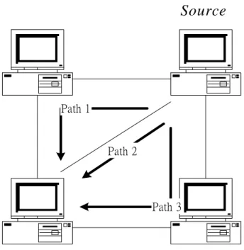
(10) Chapter 2 Survey Study of Routing Strategies Routing includes two basic phases: (1) collecting the routing information of the whole network and keeping it latest, and (2) finding a feasible path according to the routing information. In order to find an optimal path, we have to know the state information about the intervening links between source node and destination node. The way for searching feasible paths is dependent on how the state information is maintained and where the information is controlled. In this chapter there are six routing strategies including shortest path routing, separable routing, state dependent routing with trunk reservations, call admission and routing in multi-service loss networks, QoS routing for integrated services networks and hierarchical source routing using implied costs. Each above-mentioned routing strategy works based on different ideas and takes individual view of points to seek to solve the routing problem. They are classified according to how the state information is maintained and how to find their optimal paths. In the shortest-path routing, the sate information of each link is the same and it is viewed as a cost. If a link is dead, its state information changed to infinite avoiding any calls using the link. Thus calls choose the minimum-hop paths as their shortest ones. Most shortest path routing will need a distance vector protocol or a link-state protocol to maintain its global state information and will be done by hop-by-hop basis. Figure 2.1 shows a simple network. In shortest path routing, costs of path 1and path 3 are both two units. The cost of path 2 is one unit and is minimum. Hence calls from source to destination always choose path 2 if no link is dead.. 4.

(11) Source. Path 1. Path 2. Path 3. D estination Figure 2.1 Simple example for shortest-path routing.. In the separable routing [1] [2], the state information of one link is the number of calls in progress on the link. Since the state information definition and the detailed routing state information about the whole network is not tractable for computation, the state information about the whole network is simplified as the vector of link states. The cost function is also assumed separable and additive. Based on the different traffic rates flowing into individual links, each link will know when to accept or reject a new arrival in order to minimize the total blocking probability of the link (rejecting it receives a lost call now and accepting it will receive a future cost,. B ( s, λ ). B (k, λ ). , where. s is the link capacity, k is the number of calls in progress on the link and B(.,.) is Erlang-B formula. ). Suppose that a call arrives in state x and has to choose one of two available routes as followings: Route 1: direct route of link 1. Route 2: two-link route of links 2 and 3. The costs associated with the corresponding state transitions are given as follows:. Route 1: C1 =. B ( s1 , λ1 ). B ( x1 , λ1 ). . Route 2: C2 =. 5. B ( s2 , λ2 ). B ( x2 , λ2 ). +. B ( s3 , λ3 ). B ( x3 , λ3 ). ..

(12) Let C = min (C1, C2). Thus the routing rule is: If C≧1, reject the call. If C < 1, route the call on the minimum cost route. Thus source node will know if a new arrival call is sent or blocked. If a new arrival call is accepted, an optimal path will also be found. In the state-dependent routing with trunk reservations [3], a distributed, state-dependent, dynamic routing strategy called aggregated-least-busy-alternative (ALBA) is investigated. “Aggregation” means the feature wherein detailed state information is not used. Here the state information on which the routing decisions are based is the aggregate states of the links. Suppose that C+1 states representing the number of calls occupied in each link are lumped into K aggregates {A0, A1, …, Ak-1 }. Figure 2.2 shows the description of aggregate states. Parameters ri, i from 1 to k-1, are reservation parameters according to Ai-1 aggregates. The aggregation increases and the state information gets coarser with decreasing K. The special aggregate Ak-1 is the set of states with r or fewer idle circuits, where r is the trunk reservation parameter. The ALBA routing is done as follows: an arriving call is first tried on the direct route, and it is accepted if there is a free circuits. Otherwise, the call is attempted on the aggregated-least-busy two-link route. An aggregated-least-busy route for origin-destination pair i, j is one which minimizes max(Iik, Ikj) where k is an intermediate node and Iik and Ikj are the aggregate states of links (i, k) and (k, j).. Figure 2.2 Description of aggregate states In the call admission and routing for multi-service loss networks [4], the objective is maximizing the mean value of reward from the network. In order to reduce complexity, link independence is assumed and the link state information is still the number of calls in progress on the link. Thus the network reward process is decomposed of the set of link reward processes. Then the idea of the link shadow price is introduced. It is interpreted as an average price paid for carrying a call on the link. The form of the link shadow price is as follows: psj(x,π) = rsj(π) – gsj(x,π) . The link shadow price is equal to the link call reward parameter minus the expected increase in the reward from the link caused by accepting a link call. The role of the 6.

(13) price is viewed as a cost. Then it is given a negative sign and is added to the decomposed network reward process. Thus any source node finds optimal paths based on the policy of maximizing the mean value of the decomposed network reward process. In the QoS routing for integrated services networks, routing decisions are made with awareness of resource availability and requirements. Flows are routed over alternative paths with sufficiently available resources if origin paths are unable to support their requirements. This can avoid significant traffic variation in performance. In ATM networks, QoS signaling control is needed in order to set up and release resource channels. Source routing is applied. Nodes are grouped into clusters and routing domain is hierarchical to deal with traffic streams and routing information for interdomain or intradomain. In Internet, path selection is formulated as a shortest path problem for optimizing bandwidth and hop count. Three schemes are available. First, a scheme that chooses the widest-shortest path, i.e., It chooses minimum-hop path. If there are several such paths, the path with maximum residual bandwidth is chosen. Second, a scheme that chooses the shortest-widest path, it is contrast to the former. Third, a scheme that chooses the shortest-distance path. The distance is equal to the summation of the inverse of the bandwidth of links. In the hierarchical source routing using implied costs [5], such implied cost reflect the congestion in a peer group (subnetwork) and in order to represent the available capacity of the peer group the average implied cost to go through or into the group is computed. The aggregation method is that logical links have an implied cost, the, marginal cost of using this logical resource, which is approximated from the real link implied costs and two-link routing is used for aggregation in the peer group. Any broader node connects to all other nodes in the same peer group and all interdomain traffic streams are controlled by it. Finally, the goal of this routing algorithm is to maximize the rate of network revenue by adaptively adjusting splitting for each source/destination pair over time in response to changing traffic conditions. The splitting for a source/destination pair should favor routes that have a positive value of the revenue sensitivity since increasing the offered traffic on these routes will increase the rate of revenue, and on the contrary the rate of revenue will decrease.. 2.1 Strengths and weaknesses of shortest path routing. 7.

(14) In the shortest path routing, there is a ready-made routing protocol, called OSPF (Dijkstra’s shortest path algorithm). The OSPF protocol is well defined and the basic idea behind the protocol is simple: every node knows its neighbors and the totality of this knowledge is broadcasted to every node, then every node will be able to construct a complete map of the network. The shortest path routing has one serious problem. It does not support alternative paths. Since the shortest path routing only takes care about how to find a minimum-hop path, there will be some links to be overloaded if every source node takes the identical shortest path or a large amount of traffic arrival occurs unexpectedly.. 2.2 Strengths and weaknesses of Markov decision algorithms for dynamic routing (Separable routing: a scheme for state-dependent routing of circuit switched telephone traffic) The algorithms are good for designing to select routes for calls in the telephone network for real-time control of network performance, especially when the network is called upon to cope with unexpected or abnormal conditions, such as overloads, errors in load forecasts, and failures in portions of the network. Also this routing algorithm transforms the whole network state at the expense of some lost to the simpler one, the vector of link states, and allows that every link is able to control its behavior to receive an arriving call or not based on separable cost functions. Hence, it can achieve the objective of approximating the minimum value of total expected blocking probability of whole network. However, the separable still has some problems. First, although the whole network state is simplified, the global state including the network topology and the state information of every link has to be updated frequently enough to deal with the dynamics of network parameters. Once every source node updates maintained global state too frequently, it makes excessive communication overheads, especially for large scale networks. Second, the computation overhead at every source node is still high. In summary, the routing protocol has the scalability problem. In a large scale network, it is impractical. 8.

(15) 2.3 Strengths and weaknesses of state dependent routing with trunk reservations In this routing, there are several advantages. First, the detailed network state information is not used and thus the communication overhead is reduced greatly. Second, it is also a dynamic and distributed routing strategy. “Dynamic” means that an alternative path is attempted if the origin path is saturated and “distributed” means that source routing is not needed and every node will know the aggregate least-busy route to the destination. Thus the control message between source and destination is saved.. 2.4 Strengths and weaknesses of call admission and routing in multi-service loss networks First, for multiservice networks, the main contribution is synthesis of a routing strategy from an application view. Second, the important feature of this approach is the real-time traffic measurement which feed the model with the current flow distribution and provides that the control policy adapts to a time variable traffic demand, and from the modeling point of view the main contribution is the decomposition of the network reward process. Third, it is also helpful for dealing with different traffic classes (the traffic feature is classified according to how many number of required channels). Nevertheless, in this routing strategy there is no aggregation idea. The communication overhead is still high and this phenomenon is not preferred.. 2.5 Strengths and weaknesses of QoS routing for integrated services networks 9.

(16) In ATM networks, it has a hierarchy mechanism to allow scalability to large networks. A single routing protocol for the entire networks is advantageous for supporting end-to-end QoS routing and reducing the configuration associated with multiple levels of routing. It does not create any routing loops and does not result in inconsistency in the routing decision at nodes.. 2.6 Strengths and weaknesses of hierarchical source routing using implied costs The use of the hierarchical source routing is helpful for reducing communication complexity and providing acceptable QoS in a large-scale network. An approach is taken to represent the available capacity of a subnetwork. However, routes not likely to meet prespecified QoS constraints, such as end-to-end delay.. 10.

(17) Chapter 3 Background Knowledge In this chapter, three developed and time-honoured theorems or algorithms are introduced. They are continuous-time Markov decision process [6], Lagraingian multiplier [7], and maximum flow algorithm [8] respectively. The Markov decision process is used to design control actions for various link states. Lagraingian multiplier is used for a blocked cost that can be adjusted. Maximum flow algorithm is used to design our source routing algorithm.. 3.1 Continuous-time Markov decision process In this subsection, we introduce the basic idea of continuous-time Markov decision process. We call aij the transition rate of a process from state i to state j, for i ≠ j . The quantity aij is defined as follows: In a short time interval dt, a process that is now in state i will make a transition to state j with probability aij dt ( i ≠ j ) . The probability of two or more state transitions is of the order of (dt)2 or higher and is assumed to be zero if dt is taken sufficiently small. We shall consider only those processes for which the transition rates aij are constants and then describe the continuous-time Markov process by a transition rate matrix A with components aij. Note that the diagonal components have been not defined. The probability which the system occupies state i at a time t after the start of the process is the state probability πi (t). We relate the state probabilities at a time t to those a short time dt later by the equations: ⎡. ⎤. π j ( t + dt ) = π j ( t ) ⎢1 − ∑ aij dt ⎥ + ∑ π i ( t )aij dt ⎣. i≠ j. ⎦. j = 1, 2,…, N (3.1.1). i≠ j. Let us define the diagonal elements of the A matrix by a jj = −∑ a ji . If Eq. 3.1.1 i≠ j. 11.

(18) N. is used in Eg.3.1.1, we have π j ( t + dt ) − π j ( t ) = ∑ π i ( t ) aij dt . To divide both sides i =1. of this equation by dt and take the limit as dt→0, we have: N d π j ( t ) = ∑ π i ( t ) aij dt i =1. i = 1, 2, …, N (3.1.2). Equations 3.1.2 are a set of N linear constant-coefficient differential equations that relate the state probabilities to the transition-rate matrix A. If a solution is to be obtained, the initial condition π i ( 0 ) for i = 1, 2, …, N must be specified. In matrix form we can write Eqs. 3.1.2 as. d π (t ) = π (t ) A dt. (3.1.3). where π(t) is the vector of state probabilities at time t. The elements of matrix A are N. given above, and as a result the rows of A sum to zero, or. ∑a j =1. ij. = 0.. Now we define the concept of reward. Suppose that the system earns a reward at the rate of rii dollars per unit time during all the time that it occupies state i and when it makes a transition from state i to state j ( i≠j ) it receives a reward of rii dollars. It is interested to derive the expected earnings of the system that operates for a time t with a given initial condition. We let vi( t ) be the expected total reward that the system will earn in a time t starting in state i, and then we can relate the total expected reward in a time t + dt, vi( t + dt ), to vi( t ) by Eq. 3.1.4. ⎛ ⎞ vi ( t + dt ) = ⎜ 1 − ∑ aij dt ⎟ ⎡⎣ rii dt + vi ( t ) ⎤⎦ + j ≠i ⎝ ⎠. ∑ a dt ⎡⎣r j ≠i. ij. ij. + v j ( t ) ⎤⎦. (3.1.4). Eq. 3.1.4 is interpreted as follows. During the time interval dt the system maybe remains in state i or makes a transition to another state j. If it remains in state i for a time dt, it will earn a rii dt plus the expected reward that it will earn in the remaining t units of time, vi( t ). The probability that it remains in state i for a time dt is 1 minus the probability that it makes a transition in dt. On the other hand, it maybe makes a transition to some state j≠i during the time interval dt with probability aij dt. In this 12.

(19) case, the system will receive the reward rij plus the expected reward to be made starting in state j with time t remaining. We rewrite Eq. 3.1.4 as vi ( t + dt ) = (1 + aii dt ) ⎡⎣ rii dt + vi ( t ) ⎤⎦ +. ∑ a dt ⎡⎣r ij. j ≠i. ij. + v j ( t ) ⎤⎦. where terms of higher order than dt have been neglected. Finally, if we subtract vi( t ) from both sides of the equation and divide by dt, we have vi ( t + dt ) − vi ( t ) dt. N. = rii + ∑ aij rij + ∑ aij v j ( t ) j ≠i. j =1. and take the limit as dt→0, we obtain N d vi ( t ) = rii + ∑ aij rij + ∑ aij v j ( t ) dt j ≠i j =1. i = 1, 2, …, N. We have a set of N linear constant-coefficient differential equations, that completely define vi( t ) when the vi(0) are known. Let us define a quantity qi as the “earning rate” of the system where qi = rii + ∑ aij rij . j ≠i. For a given policy the total expected reward of the system in time t is governed by Eqs. 3.1.5 N d vi ( t ) = qi + ∑ aij v j ( t ) dt j =1. i = 1, 2, …, N (3.1.5). Since we are concerned only with processes whose termination is remote, we may use the asymptotic expression (Eq. 3.1.6) for vi( t ) vi( t ) = tgi + vi for large t. (3.1.6). and transform Eqs. 3.1.5 into gi = qi + ∑ aij ( tg j + v j ) N. j =1. 13. (3.1.7).

(20) If Eqs. 3.1.7 are to hold for all large t, then we obtain the two sets of linear algebraic equations N. ∑a g j =1. ij. j. =0. i = 1, 2,…, N (3.1.8). N. gi = qi + ∑ aij v j i = 1, 2,…, N (3.1.9) j =1. Solution of Eqs. 3.1.8 expresses the gain of each state in terms of the gains of the recurrent chains in the process. The relative value of one state in each chain is set equal zero, and Eqs. 3.1.9 are used to solve for the remaining relative values and the gains of the recurrent chains. Suppose that we have a policy that is optimal when t units of time remain, and that this policy has expected total rewards vi( t ). If we are considering what policy to follow if more time than t is available, we see from Eqs. 3.1.5 that we may maximize our rate of increase of vi( t ) by maximizing N. qik + ∑ aij k v j ( t ). (3.1.10). j =1. with respect to the alternatives k in state i. If t is large, we may use vj( t ) = tgj + vj. to obtain N. N. j =1. j =1. qik + ∑ aij k v j + t ∑ aij k g j. (3.1.11). as the quantity to be maximized in the ith state. For large t, Expression 3.1.11 is maximized by the alternative that maximizes N. ∑a j =1. ij. k. (3.1.12). gj. the gain test quantity, using the gains of the old policy. However, when all alternatives produce the same value of Expression 3.1.12 or when a group of alternatives produces the same maximum value, then the tie is broken by the alternative that maximizes. 14.

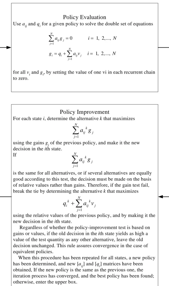
(21) N. qik + ∑ aij k v j. (3.1.13). j =1. the value test quantity, using the relative values of the old policy. The relative values may be used for the value test because a constant difference will not affect decisions within a chain. The general iteration cycle is shown in Figure 3.1. It, as is usually the case, all possible policies of the problem are completely ergodic, the computational process may be considerably simplified. Since all states of each Markov process have the same gain g, the value-determination operation involves only the solution of the equations N. g = qi + ∑ aij v j. i = 1, 2,…, N (3.1.14). j =1. with vN set equal to zero. The solution for g and the remaining vi is then used to find an improved policy. Multiplication of Eqs. 3.1.14 by the limiting state probability πi and summation over i show that N. g = ∑ π i qi i =1. a result previously obtained. The policy-improvement routine becomes simply: For each state i, find the alternative k that maximizes N. qi k + ∑ aij k v j j =1. using the relative values of the previous policy. This alternative becomes the new decision in the ith state. A new policy has been found when this procedure has been performed for every state. The iteration cycle for completely ergodic continuous-time systems is shown in Figure 3.2. Note that, if the iteration is started in the policy-improvement routine with all vi = 0, the initial policy selected is the one that maximizes the earning rate of each state.. 15.

(22) Policy Evaluation Use aij and qi for a given policy to solve the double set of equations N. ∑a j =1. ij. gj = 0. i = 1, 2,..., N. N. g i = qi + ∑ aij v j. i = 1, 2,..., N. j =1. for all vi and gi, by setting the value of one vi in each recurrent chain to zero.. Policy Improvement For each state i, determine the alternative k that maximizes N. ∑a. k. ij. j =1. gj. using the gains gj of the previous policy, and make it the new decision in the ith state. N If k. ∑a j =1. ij. gj. is the same for all alternatives, or if several alternatives are equally good according to this test, the decision must be made on the basis of relative values rather than gains. Therefore, if the gain test fail, break the tie by determining the alternative k that maximizes N. qi + ∑ aij k v j k. j =1. using the relative values of the previous policy, and by making it the new decision in the ith state. Regardless of whether the policy-improvement test is based on gains or values, if the old decision in the ith state yields as high a value of the test quantity as any other alternative, leave the old decision unchanged. This rule assures convergence in the case of equivalent policies. When this procedure has been repeated for all states, a new policy has been determined, and new [aij] and [qi] matrices have been obtained, If the new policy is the same as the previous one, the iteration process has converged, and the best policy has been found; otherwise, enter the upper box.. Figure 3.1 General iteration cycle for continuous-time decision processes.. 16.

(23) Value-Determ ination Operation Use a ij and q i for a given policy to solve the set of equations N. g = q i + ∑ a ij v j. i = 1, 2,..., N. j =1. for all relative values v i and g by setting v N to zero.. Policy-Im provem ent Routine For each state i, find the alternative k that m axim izes N. q i k + ∑ a ij k v j j =1. using the relative values v i of the previous policy. Then k’ becom es the new decision in the ith state, q ik ’ becom es q i, and a ijk ’ becom es a ij.. Figure 3.2 Iteration cycle for completely ergodic continuous-time decision processes.. 3.2 Lagrangian multiplier The classic technique for dealing with constrained maximization problems is the method of Lagrangian multipliers. A constrained maximization problem is that one wishes to maximize a function f (x) over some set of x-values X, subject to the constraint g(x) = b.. (3.2.1). If there are several constraints, then g and b must be regarded as vectors. The commonest example in an economic-technical context is that of allocation, when x represents a pattern of activity (such as the amounts of various goods which are to be manufactured), f(x) the consequent economic return, g(x) the consequent consumption of necessary resources (such as capital, labour, raw materials, energy, etc.) and b the amounts of these resources available. Actually, for this example one should rather modify the constraint (3.2.1) to g(x) ≦ b. (3.2.2). since there is usually no compulsion to exhaust all resources. 17.

(24) The method of Larangian multipliers is based on the fact that, if xˆ is a value in X maximizing f(x) subject to (3.2.1), then under some conditions, there exits a multiplier vector y with property that the form f(x) - yTg(x) is stationary at x = xˆ . This assertion, when true, we shall refer to as the weak or classical Lagrangian principle. Under certain conditions a stronger conclusion can be deduced: that xˆ maximizes the Lagrangian form f(x) - yTg(x) absolutely in X. This assertion, when true, we shall refer to as the strong Lagrangian principle. The simple nature of the strong principle obviously makes it attractive. For instance, there is no mention of derivatives and, indeed, the principle may hold in cases when f(x) or g(x) do not possess derivatives at xˆ (although compensating conditions of some other nature are required). Neither does the fact that xˆ may be a boundary point of X affect the statement of the principle. Both Lagrangian principles can be adapted to the case of inequality constraints such as (3.2.2), or indeed, to very much more general forms of constraint. Suppose that the point xˆ + ε s , where ε is a non-negative scalar and s a vector, belongs to X for all non-negativeε less than some positive valueε(s). Then s will be described as directed into the interior of X from xˆ , or as a feasible direction from xˆ . Denote the row vector of derivatives ⎡ ∂f ∂f ∂f ⎤ , ,..., ⎢ ⎥ ∂xn ⎦ ⎣ ∂x1 ∂x2. if this exits, by fx. If the derivative fx exists at xˆ , then fxs ≦ 0 at xˆ for feasible directions s from xˆ . In particular, if xˆ is an interior point of X, then fx = 0. (3.2.3). at xˆ . Criterion (3.2.3) is the classic stationary condition, the condition that xˆ be a stationary point of f. For the weak Lagrangian principle, an appropriate stationary point of the Lagrangian form is located, and y is then adjusted until the constraint (3.2.1) is satisfied at the stationary point.. 3.3. Maximum Flow Algorithm. 18.

(25) Network flow problems are linear programs with the particularly useful property that they posses optimal solutions in integers. In this subsection we review “classical” network flow theory, including the max-flow min-cut theorem and computation of minimum cost flows. Suppose that each arc (i, j) of a directed graph G has assigned to it a non-negative number cij, the capacity of (i, j). The capacity can be thought of as representing the maximum amount of some commodity that can “flow” through the arc per unit time in a steady-state situation. Such a flow is permitted only in the indicated direction of the arc, i.e., from i to j. Consider the problem of finding a maximal flow from a source node s to a sink node t, which can be formulated as follows. Let xij = the amount of flow through arc (i, j). Then, 0 ≦ xij ≦ Cij.. (3.3.1). A conversation law is observed at each of the nodes other than s or t. That is, what goes out of node i must be equal to what comes in. So we have ⎧ −v, i = s ⎪ ∑j x ji − ∑j xij = ⎨0, i ≠ s, t ⎪v, i = t . ⎩. (3.3.2). We call any set of numbers x = (xij) which satisfy (3.3.1) and (3.3.2) a feasible flow, or simply a flow, and v is its value. The problem of finding a maximum value flow from s to t is a linear program in which the objective is to maximize v subject to constraints (3.3.1) and (3.3.2). Let P be an undirected path from s to t. An arc (i, j) in P is said to be a forward arc if it is directed from s toward t and backward otherwise. P is said to be a flow augmenting path with respect to a given flow x = (xij) if xij < cij for each forward arc (i, j) and xij > 0 for each backward arc in P. A (s, t)-cutset is identified by a pair (S, T) of complementary subsets of nodes, with s ∈ S and t ∈ T. The capacity of the cutset (S, T) is defined as. 19.

(26) c ( S , T ) = ∑∑ cij , i∈S j∈T. i.e., the sum of the capacities of all arcs which are directed from S to T. The value of any (s, t)-flow cannot exceed the capacity of any (s, t)-cutset. Suppose that x = (xij) is a flow and (S, T) is an (s, t)-cutset. Sum the equations (3.3.2) identified with nodes i ∈ S to obtain ⎛ ⎞ v = ∑ ⎜ ∑ xij − ∑ x ji ⎟ i∈S ⎝ j j ⎠. = ∑∑ ( xij − x ji ) + ∑∑ ( xij − x ji ) i∈S j∈S. (3.3.3). i∈S j∈T. = ∑∑ ( xij − x ji ) i∈S j∈T. That is, the value v of any flow is equal to the net flow through any cutest. But xij ≦ cij and xji ≧ 0, so v ≤ ∑∑ cij = c ( S , T ) i∈S j∈T. It follows that from the preceding analysis that the flow is maximal and that the cutest has minimal capacity. Notice that each arc (i, j) is saturated, i.e., xij = cij, if i∈S, j∈T and void, i.e., xij = 0, if i∈T, j∈S. We now state three of the principle theorems of network flow theory. They will later be applied to yield good algorithms for maximal flow problems. Theorem (Augmenting Path Theorem) augmenting path from s to t. Theorem (Integral Flow Theorem) maximal flow which is integral.. A flow is maximal if and only if it admits no. If all arc capacities are integers there is a. Theorem (Max-Flow Min-Cut Theorem) The maximum value of an (s, t)-flow is equal to the minimum capacity of an (s, t)-cutset.. The problem of finding a maximum capacity flow augmenting path is evidently 20.

(27) quite similar to the problem of finding a shortest path, or, more precisely, a path in which the minimum arc length is maximum. We can make the similarity quite clear, as follows. Let. cˆij = max {cij − xij , x ji } ,. where cij = 0, if there is no arc (i, j). Let ui = the capacity of a maximum capacity augmenting path from node s to node i. Then the analogues of Bellman’s equations are: us = +∞. ui = max min {uk , cki } k. i ≠ s.. It is clear that the ui values and the corresponding maximum capacity paths can be found by Dijkstra-like computation which is O(n2). Actually, we shall be satisfied with a computation which does not necessarily compute maximum capacity paths. A procedure in which labels are given to nodes is proposed. These labels are of the form (i+, δj) or (i-, δj). A label (i+, δj) indicates that these exists an augmenting path with capacityδj from the source to the node j in question, and that (i, j) is the last arc in this path. A label (i-, δj) indicates that (j, i) is the last arc in the path, i.e., (j, i) will be a backward arc if the path is extended to the sink t. Initially only the source node s is labeled with the special label (-, ∞ ). Thereafter, additional nodes are labeled in one of two ways: If node i is labeled and there is an arc (i, j) for which xij < cij, then the unlabeled node j can be given the label (i+, δj), where. δ j = min {δ i , cij − xij } .. If node i is labeled and there is an arc (j, i) for which xji > 0, then the unlabeled node j can be given the label (i-, δj), where. δ j = min {δ i , x ji } .. 21.

(28) When the procedure succeeds in labeling node t, an augmenting path has been found and the value of the flow can be augmented by δt . If the procedure concludes without labeling node t, then no augmenting path exists. A minimum capacity cutest (S, T) is constructed by letting S contain all labeled nodes and T contain all unlabeled nodes. A labeled node is either “scanned” or “unscanned.” A node is scanned by examining all incident arcs and applying labels to previously unlabeled adjacent nodes, according to the rules given above. The maximal flow algorithm is shown as follows: Step 0 (Start) Let x = (xij) be any integral feasible flow, possibly the zero flow. Give node s thee permanent label (-, ∞ ).. Step 1 (Labeling and Scanning) (1.1) If all labeled nodes have been scanned, go to Step 3. (1.2) Find a labeled but unscanned node i and scan it as follows: For each arc (i, j), if xij < cij and j is unlabeled, give j the label (i+, δj), where. δ j = min {cij − xij , δ i } For each arc (j, i), if xji > 0 and j is unlabeled, give j the label (i-, δj), where. δ j = min { x ji , δ i } .. (1.3). If node t has been labeled, go to Step 2; otherwise go to Step 1.1.. Step 2 (Augmentation) Starting at node t, use the index labels to construct an augmenting path. (The label on node t indicates the second-to-last node in the path, the label on that node indicates the third-to-last node, and so on.) Augment the flow by increasing and decreasing the arc flows byδt , as indicated by the superscripts on the index labels. 22.

(29) Erase all labels, except the label on node s. Go to Step 1.. Step 3 (Construction of Minimal Cut) The existing flow is maximal. A cutset of minimum capacity is obtained by placing all labeled nodes in S and all unlabeled nodes in T. The computation is completed.. 23.

(30) Chapter 4 Proposed Scheme In this chapter, first we will formulate this routing problem to the constrained Markov decision process, and find the optimal policy (the partitions on each link) corresponding to the value of Lagrangian multiplier called Lambda here by using value determine and policy improvement procedure. Second, the original maximum flow algorithm is modified and we will describe our modified algorithm at each source node for choosing the best feasible route or the shortest-path to avoid more calls lost in the future when a new call is arriving.. 4.1. Link State Aggregation. We describe the network as a set of nodes N and a set of links K connecting the nodes. Hence K=1, 2, …, 1/2N(N-1) . Any call attempt of type k∈K will be a call attempt with the link k. The link k contains Ck ≧0 trunks. In this subsection, we first make some assumptions below. Suppose that the network is offered only one class of call and operates in a lost call model. That is, in our network, all arriving calls will request the same number of occupied trunks which we give the unit trunk the value of 1, and if a arriving call is blocked, no retransmission will happen and it will be cleared. When a call is accepted we assume that the setup of a call is instantaneous. In treating traffic routing as Markov decision process and obtaining the cost to carry a connection by the network in the light of the Markov decision theory, the network state will require the detailed specification of the number of calls in processing on each feasible path. Because of enormous computations of the network state, network state should be approximated to a simpler definition for practical implementation. Some assumptions are made based on previous researches: statistical link independence and separable cost. First, link independence assumes that when a call is routed on a multi-link route, the call will be set up n independent calls with independent, identically distributed holding times and also they terminate independently. The call holding time for each call is exponentially distributed with the same mean, µ −1 , which is used as the unit of time and given the value 1. This 24.

(31) assumption is needed in order to reduce the routing information from the specification of the whole network to the specification of one trunk group. Second, separable cost assumes that the cost of carrying a call over a route is the sum of the cost of carrying a directed-link call over each link of the route respectively. The further reduced state information is helpful to heal the enormous computation. By assumptions above in the network, the network state is decomposed of the vector of link states. Each link state is described by the description of occupied trunk over the link. The call arrivals for different origin-destination pairs are traffic streams which follow the independent Poisson distribution, and the possibility of blocking a call followed by accepting a call on condition of the same link depends on the value of the call arrival rate on the link, i.e. on condition of accepting a call higher arrival rate makes more lost probability of calls continued. It is important for each link to compute its cost by knowing two arguments: the current state of the link and that how many calls will be set up over itself by node pairs in the future. Once the link considers that the cost of accepting a call continuously is higher than the one of blocking a call, the link should notify nodes that send traffic over it with the latest routing information that the link is overloaded or congested. Such the latest exchanged information will result in much network overhead. Instead of the precise routing information, if a coarse one is replaced for cost computing, the computed cost is not accurate and overall expected blocking probability of each link will increase. In the large network if the link information is flooding through the whole network instantaneously once the link state is changed, although source nodes will receive the accurate routing information for making decisions but simultaneously the network will be congested resulting from a great amount of flooding. This phenomenon is not preferred for us. Our state aggregation method is the following. First, we define the cost function. Upon accepting a call, the system obtains a reward 1. The system will receive a lossλ if blocking a call. By using strong Largrangian principle under the stationary condition, we maximize the function: E[ Rt ] – λ * b Rt is the received reward from time t to t+1. b is the blocking probability of the link. From strong Largragian principle, we can find the value ofλto let the value of b less than 0.1. Our goal is to let each link with the blocking probability less than 0.1 if it is possible and to go back to shortest-path routing if it is not possible. The value 0.1 can 25.

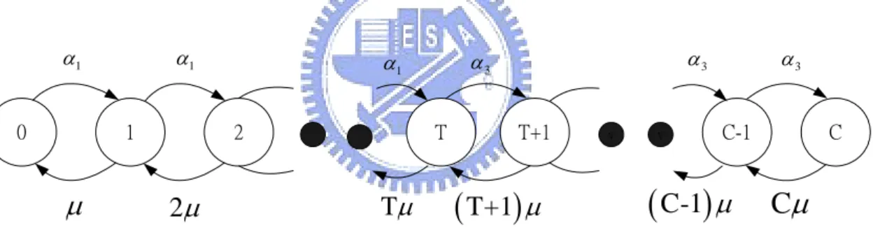
(32) be modified according to different requirements. Here the use of the strong Largrangian principle is intuitive. We recall that the definition of one link state is the number of calls in progress on the link originally in MDP routing. We aggregate them into three congestion levels and an advertisement information is delivered to each router when the state transit to another different congestion level. Let αi be the maximum arrival rate during the congestion level i and the inequalityα1<α2<α3 is assumed. The advertisement is that the link notifies each router its maximum arrival rateαi during the congestion level i. Then the MDP formulation can be used. By the formulation we observe that α2 is a mixing policy of α1 and α3 , but there exists a deterministic optimal policy. In other words, we can think that the behavior of the link is divided two parts which are congested and non-congested, and it can be represented for handling all traffic conditions. We know that only two congestion levels are enough and then three or above congestion levels can be decreased to two levels. Thus the state transition diagram is shown as follows. α1. α1. µ. T. 2. 1. 0. 2µ. α3. α3. α1. Tµ. T+1. ( T+1) µ. v. v. α3 C. C-1. ( C-1) µ. Cµ. Figure 4.1. State transition diagram for two congestion levels In this figure, we suppose that in this network there are C trunks in each link totally and T is the threshold state between two congestion levels. The low congestion level consists state 0 ~ T-1 and the high congestion level consists state T ~ C. We design that T will be modified according to the blocking probability of the previous time interval. It is shown below: T = T + 1, if bs < 0.1. T = T – 1, otherwise. Here bs is the blocking probability of previous sample time interval.. 4.2 Node Maxflow source routing algorithm 26.

(33) In this subsection, we describe the source routing mechanism for choosing a best one from feasible paths in the Node. Based on the Maximum Flow Algorithm, in the beginning for each link the value λ1 (we mentioned above) is used as the maximum amount of calls that can flow through it per unit time in the steady-state situation. Then we can find the maximum flow, a maximum capacity flow augmenting path, and other feasible flow paths. If any link broadcasts its routing information and changes the maximum amount of calls that can flow through it per unit time now, the maximum flow and flow paths are immediately computed again. Before the algorithm, we denote some parameters below for discussion later: rs: the source traffic rate. fbs: the flow rate that a call blocked in the source. That if it is not zero is meant to block a call according to fbs / rs at source nodes. Here we do not hope to block any calls at source nodes instead of delivering calls through the shortest path. The reason we choose the shortest path under this situation is that choosing one from feasible flow paths results in occupying resources on more links. fmax: the total maximum flow. cmax: the maximum capacity of a maximum capacity flow augmenting path. randNr: a random number which the value is between 0 and 1. The routing algorithm we proposed is below: if ( rs > fmax ) fbs = rs – fmax ; else fbs = 0 ; if ( randNr ≧ fbs / rs ) { if ( rs ≦ cmax ) choose the maximum capacity flow augmenting path; else choose one from all feasible paths randomly ; } else choose the shortest path ; Now we illustrate the operation of our algorithm. First, if the source traffic rate is greater than the total maximum flow, it shows that the network is not capable of this source traffic and it is preferred to block the exceeded amount of source traffic in the source. Thus we take fbs / rs as the average blocking probability in the source on arriving a new call. Second, if the call is not blocked in the source, the maximum capacity flow augmenting path is checked if it will be used. That rs ≦ cmax means the maximum capacity flow augmenting path can still load the source traffic, or we have 27.

(34) to randomly choose one path from all feasible ones while a new call is originated. This algorithm is represented as a flow chart as follows: ( else ) Choose one path from all feasible flow paths randomly Generates calls. ( If rs <= cmax ) choose maximum capacity flow augmenting path Check if there is any traffic blocked at source ? ( If randomNr < fbs / rs ) choose shortest path. ( Yes ) fbs = rs - fmax. ( No ). fbs = 0. Choose flow augmenting path ?. Generates a random number randNr :[0,1]. Choose path ?. ( else ). Figure 4.2. Flow chart of the Maxflow source routing algorithm. Chapter 5 28.

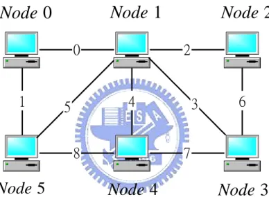
(35) Numerical Results In this chapter, performance of Maxflow source routing with various call arrival rates is evaluated via simulations and compared with performance of shortest path routing. Also the communication overhead of Maxflow source routing is computed for scalable test. Here we take a simple example of a small network. Figure 5.1 shows the network example for our simulation.. Node 1. Node 0 0. 1. 2. 4. 5 8. Node 5. Node 2. 3. 6. 7. Node 4. Node 3. Figure 5.1. An example of a simple network There are six nodes and nine links in this network example that is not fully connected. The Nodes are the notions of “computer” above, and the links are black lines with a number ID used for the ID of trunk group. Each node with any other node will form a origin-destination pair for transmitting calls. In our simulation, the capacity of each link is 30 trunks and the network only support one class of traffic, which bandwidth requirement is one trunk. Despite of Node 5, any other nodes are attempted to carry calls with some arrival rate to Node 5. Thus all OD pairs in this situation are as follows:. ( origin, destination ) : ( 0,5) , (1,5 ) , ( 2,5 ) , ( 3,5) , ( 4,5) In other words, Node 5 is a destination node but not a source node. That the arrival rate of traffic is assumed the same at all source nodes in one experiment is designed to 29.

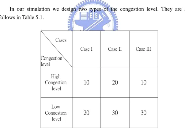
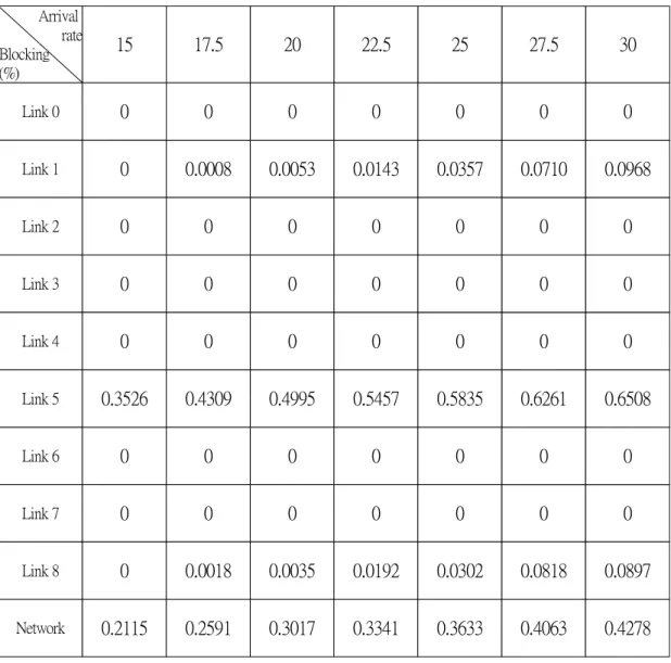
(36) verify experiments under different arrival rates. The rates we chosen after are 15, 17.5, 20, 22.5, 25, 27.5 and 30. Table 5.2 shows the result under different arrival rates when shortest path routing is used at each source node to elect minimum-hop routes for calls. This table shows that in this situation there are three critical links, which are Link 1, 5, 8. Among these critical links, the blocking probability of calls on Link 5 is very higher than ones of calls on Link 1 and Link 8. The reason for the higher probability is that Node 1, 2, and Node 3 all attempt to carry their traffic streams into Link 5 since the shortest path routing is used. Link 1 and Link 8 are loaded traffic streams of Node 0 and Node 4 respectively. (The shortest path of the OD pair (2, 5) is two-link path including Link 2 and Link 5. Also the shortest path of the OD pair (3, 5) is two-link path including Link 3 and Link 5.) This phenomenon is to explain why the shortest path routing is not always useful. With shortest path routing algorithm it is possible for carrying too many calls on some critical link to increase the blocking probabilities of the link and overall network. In our simulation we design two types of the congestion level. They are as follows in Table 5.1.. Cases Case I. Case II. Case III. High Congestion level. 10. 20. 10. Low Congestion level. 20. 30. 30. Congestion level. Table 5.1 Types of congestion level. Table 5.3 shows one result for Case I under different arrival rates when Maxflow source routing is applied at each source node to elect a suitable path for calls under different network routing information. This Table shows that for overall network using Maxflow source routing has less blocking probability than using shortest path 30.

(37) routing under any different arrival rates. Although with Maxflow source routing Link 1 and Link 8 have higher blocking probability than ones with shortest path routing, using Maxflow source routing make Link 5 lower blocking than using shortest path routing. This fully explains that originally with shortest path routing a portion of calls from Link 5 changes to Link 1 or Link 8 since Maxflow source routing is used. It is desired for decreasing overall network blocking probability as low as possible. It is obvious in our experiment that for the compare of blocking probability on Link 5 under traffic rate 20 and 22.5 or traffic rate 17.5 and 20. Especially the difference of the blocking probability on Link 5 for traffic rate 17.5 and 20 exceeds twenty percent. Besides, the parameter for advancing or reducing threshold is designed as 0.1, i.e., if in a length of time interval the blocking probability of the link is greater than 0.1, the threshold is advanced one until threshold is equal to 30, and threshold is reduced one if the probability is equal or lower than 0.1. This design is not clear under traffic rate above 20 because the rate is too high to overload some links still. Table 5.4 and Table 5.5 show other results for Case II and Case III under different arrival rates when Maxflow source routing is applied at each source node to elect a suitable path for calls under different network routing information. Equally, the designs of congestion level for Case II and for Case III decrease overall network blocking probability compared with one of shortest path routing. The difference among link probabilities between Case I and Case II is that for Case II the blocking rate of Link 5 is more reduced and the blocking rates of Link 1 and Link 8 are higher. The behavior of Case III is like the one of Case I because they are only different in the design of the low congestion level. Figure 5.2 shows that the compare for overall network blocking probability under various traffic arrival rates between shortest path routing and Maxflow source routing (Case I, Case II, and Case III). It is clear that the network blocking probability of shortest path routing decreases as the arrival rate decreases almost with a fixed slope. For Case I, the network blocking probability of Maxflow source routing from traffic rate 30 to 22.5 is like the behavior of shortest path routing with almost the same slope but with a lower blocking rate. Then from traffic rate 20 to 15, the network blocking probability decreases rapidly at a very oblique angle. Our illustration is that for traffic rate above 20, it makes critical links congested frequently and thus source nodes have higher possibility to choose shortest paths. For traffic rate equal to or below 20, Maxflow source routing works well because source nodes have 31.

(38) less possibility to choose shortest paths. Particularly the differences of network blocking between Maxflow source routing and shortest path routing under traffic rates 17.5 and 15 are twenty percent and upward. For Case II and Case III, the behaviors of overall network blocking probability are similar to the one of Case I. Some difference between them is the following. The blocking probabilities of Case II from traffic rate 25 to rate 30 are all a little higher than ones of Case I. The reason is that the high congestion level of Case II is higher than the one of Case I. It makes congested links accepting more traffic streams continuously. We run our simulation under various traffic rates according to different multipliers and observe that blocking probabilities of links and network are independent of different multipliers over a long period of time. This observation shows that the long-term behaviors of network and links will converge toward the same result although the initial multiplier value is different. Finally, Table 5.6 shows the computation of link update overheads for scalability test. Here we list average overhead value and maximum deviation overhead value according to three cases under various arrival rates. First, we can see that the average values for traffic rates 15, 17.5 and 20 are higher than others. Especially, the value for traffic rate 17.5 is almost equal to one, and this means that the link routing information will be updated one time per second averagely. Luckily it is acceptable since the link will equally broadcast its link information 0.33 times per second for that total overheads is distributed into three critical links. The reason of smaller value for traffic rate from 22.5 to 30 is that critical links under these traffic rates frequently attempt to notify source nodes that it is in the high congestion level. Thus in this situation the communication overhead will be lightened. Second, for Case III the value of link update under traffic rate 17.5 is highest. If the value 1.6905 is distributed into three critical links, each critical link floods its link routing information to overall network every two seconds almost. Thus it shows an acceptable situation. In the low-congested traffic condition, it remains a higher overhead value, and in the high-congested traffic condition, it decreases to a lower overhead value.. 32.

(39) Arrival rate Blocking (%). 15. 17.5. 20. 22.5. 25. 27.5. 30. Link 0. 0. 0. 0. 0. 0. 0. 0. Link 1. 0. 0.0008. 0.0053. 0.0143. 0.0357. 0.0710. 0.0968. Link 2. 0. 0. 0. 0. 0. 0. 0. Link 3. 0. 0. 0. 0. 0. 0. 0. Link 4. 0. 0. 0. 0. 0. 0. 0. Link 5. 0.3526. 0.4309. 0.4995. 0.5457. 0.5835. 0.6261. 0.6508. Link 6. 0. 0. 0. 0. 0. 0. 0. Link 7. 0. 0. 0. 0. 0. 0. 0. Link 8. 0. 0.0018. 0.0035. 0.0192. 0.0302. 0.0818. 0.0897. Network. 0.2115. 0.2591. 0.3017. 0.3341. 0.3633. 0.4063. 0.4278. Table 5.2. Blocking probabilities of shortest path routing under various arrival rates.. 33.

(40) Arrival rate Blocking (%). 15. 17.5. 20. 22.5. 25. 27.5. 30. Link 0. 0. 0. 0.0798. 0.0942. 0.0972. 0.0988. 0.0999. Link 1. 0.0073. 0.0592. 0.0956. 0.1177. 0.1873. 0.2534. 0.3178. Link 2. 0. 0. 0.0261. 0.0052. 0.0082. 0.0090. 0.0132. Link 3. 0.0007. 0.0021. 0. 0. 0. 0. 0. Link 4. 0. 0. 0.0002. 0. 0. 0. 0.0003. Link 5. 0.0063. 0.0537. 0.2685. 0.4310. 0.4547. 0.4903. 0.5324. Link 6. 0.0038. 0.0241. 0.0131. 0.0006. 0.0015. 0.0002. 0.0002. Link 7. 0. 0. 0. 0. 0. 0. 0. Link 8. 0.0084. 0.0524. 0.0997. 0.1040. 0.1473. 0.1672. 0.2074. Network. 0.0083. 0.0581. 0.1853. 0.2730. 0.3107. 0.3491. 0.3964. Table 5.3. Blocking probabilities of Maxflow source routing using Case I under various arrival rates.. 34.

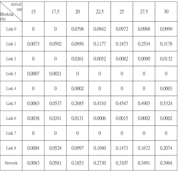
(41) Arrival rate Blocking (%). 15. 17.5. 20. 22.5. 25. 27.5. 30. Link 0. 0. 0.0046. 0.0311. 0.1528. 0.1993. 0.2174. 0.2559. Link 1. 0.0053. 0.0696. 0.0992. 0.2912. 0.3464. 0.4103. 0.4714. Link 2. 0. 0.0153. 0.0544. 0.0961. 0.0968. 0.1004. 0.1019. Link 3. 0.0016. 0.0015. 0. 0. 0.0043. 0.0003. 0.0029. Link 4. 0. 0. 0. 0. 0. 0. 0. Link 5. 0.0106. 0.0784. 0.1934. 0.1149. 0.1248. 0.1614. 0.1870. Link 6. 0.0036. 0.0739. 0.0997. 0.0956. 0.0962. 0.0989. 0.1044. Link 7. 0. 0. 0. 0.0096. 0.0038. 0.0024. 0.0029. Link 8. 0.0153. 0.0922. 0.0975. 0.2419. 0.3098. 0.3731. 0.4323. Network. 0.0120. 0.0962. 0.1642. 0.2722. 0.3180. 0.3696. 0.4201. Table 5.4. Blocking probabilities of Maxflow source routing using Case II under various arrival rates. 35.

(42) Arrival rate Blocking (%). 15. 17.5. 20. 22.5. 25. 27.5. 30. Link 0. 0. 0. 0.0867. 0.0932. 0.0980. 0.0982. 0.1003. Link 1. 0.0054. 0.0513. 0.0990. 0.1137. 0.1967. 0.2912. 0.3358. Link 2. 0. 0.0002. 0.0048. 0.0081. 0.0187. 0.0131. 0.0244. Link 3. 0.0003. 0.0009. 0.0039. 0.0091. 0.0301. 0.0327. 0.0494. Link 4. 0. 0. 0.0002. 0. 0. 0.0007. 0. Link 5. 0.0109. 0.0788. 0.3136. 0.4087. 0.4466. 0.5057. 0.5306. Link 6. 0. 0. 0. 0. 0. 0. 0. Link 7. 0. 0. 0. 0. 0. 0. 0. Link 8. 0.0036. 0.0407. 0.0971. 0.1005. 0.1231. 0.1768. 0.2143. Network. 0.0063. 0.0565. 0.2017. 0.2614. 0.3086. 0.3710. 0.4046. Table 5.5. Blocking probabilities of Maxflow source routing using Case III under various arrival rates. 36.

(43) Shortest-Path Routing Maxflow Source Routing - Case I Maxflow Source Routing - Case II Maxflow Source Routing - Case III 0.4278. 0.45 0.4063 0.4. 0.371 0.3696. 0.3633 0.3341. 0.35. 0.3107 0.3086. 0.3 Network Blocking (%). 0.3491. 0.318. 0.3017 0.273. 0.2591. 0.4201 0.4046 0.3964. 0.25 0.2115. 0.2722 0.2017. 0.2. 0.2617. 0.1853 0.1642. 0.15. 0.1. 0.0962. 0.05. 0.0581 0.0565. 0.012 0 15. 0.0083 0.0063 17.5. 20. 22.5. 25. 27.5. 30. Arrival Rate. Figure 5.2. Network Blocking Comparison for shortest path routing and Maxflow source routing. 37.

(44) Average (/sec). Deviation (/sec). Arrival Rate. Case I. Case II. Case III. Case I. Case II. Case III. 15. 0.5520. 0.5886. 0.5172. 2.7. 2.7. 2.6. 17.5. 0.9704. 1.0342. 0.9550. 4.1. 4.2. 3.5. 20. 0.6641. 1.6905. 0.5665. 3.4. 4.5. 3.0. 22.5. 0.2520. 0.2796. 0.2797. 2.5. 2.2. 2.4. 25. 0.2563. 0.2160. 0.3095. 1.6. 1.7. 2.8. 27.5. 0.2731. 0.2579. 0.3657. 2.7. 2.0. 3.3. 30. 0.2880. 0.1402. 0.3904. 1.7. 1.5. 2.0. Table 5.6. Computation of Link Update Overheads. 38.

(45) Chapter 6 Conclusion State-dependent routing is preferred for the real-time control of network performance in the past. It needs to use the network state information in order to select a route for a call. In this work, we study various routing strategies including shortest-path routing, QoS routing, and other state-dependent routing strategies with different objectives and ideas. Based on the above learning and other background knowledge, we propose an aggregation scheme and a source-based routing algorithm to provide network scalability. In our simulation we run the MDP function on links to aggregate routing information for providing network scalability and design the Maxflow source routing algorithm as the source routing algorithm used at source nodes. The MDP function is used for partitioning the congestion level sets of each link. The Maxflow source routing algorithm chooses the appropriate routes according to above-mentioned congestion information of each link. Based on these ideas, we can decrease the network probability that results from shortest path routing greatly and reduce the number which links flood their routing information into overall network as few as possible. As the simulation result shown, the Maxflow source routing is superior to shortest-path routing.. 39.

(46) References [1] Teunis J. OTT and K. R. Krishnan, “Separable Routing: A Scheme for State-Dependent Routing of Circuit Switched Telephone Traffic”, Annals of Operations Research, Volume 35, Issue 1-4, pp.43-68, April 1992. [2] K. R. Krishnan, “Markov Decision Algorithms for Dynamic Routing’, IEEE Communications Magazine, 28:10, 66-69. [3] Debasis Mitra, Richard J. Gibbens, and Baosheng D Huang, “State-Dependent Routing on Symmetric Loss Networks with Trunk Reservations-I”, IEEE Transaction. Communications, Volume 41, No. 2, February 1993. [4] Zbigniew Dziong, and Lorne G. Mason, “Call Admission and Routing in Multi-Service Loss Networks”, IEEE Transaction. Communications, Volume 42, No 2/3/4, February/March/April 1994. [5] Michael Montgomery and Gustavo De Veciana, “Hierarchical Source Routing using Implied Costs”, Computer Networks: The International Journal of Computer and Telecommunications Networking, Volume 34, Issue 3, pp. 379-397, September 2000. [6] Ronald A. Howard, “Dynamic Programming and Markov Process”, The MIT Press, (June 15, 1960). [7] Peter Whittle, “Optimization under Constraints: Theory and Applications of Nonlinear Programming”, A Wiley-Interscience Publication. [8] Eugene Lawler, ”Combinatorial optimization : Network and Matroids”, Dover Publications (March 2, 2001). [10] Ben-Jye Chang and Ren-Hung Hwang, “Hierarchical QoS routing in ATM networks based on MDP cost function”, IEEE ICON 2000, pp.147-151, Sep. 2000. [11] Larry L. Peterson and Bruce S. Davie, “Computer Networks: A Systems Approach”, Edition 3, Boston: Morgan Kaufmann Publishers 2003.. 40.

(47) [12] F. P. Kelly, “Routing in Circuit-Switched Networks: Optimization, Shadow Prices and Decentralization”, Adv. Annals of Applied Probability. Prob. 20, pp. 112-144, 1988. [13] William Stallings, “High-Speed Networks and Internets: Performance and Quality of Service”, Prentice Hall; 2 edition (January 15, 2002).. 41.

(48)