表面吸附分子的轉動能態及量子點的電子性質之研究

國

立

交

通

大

學

電子物理研究所

博 士 論 文

表面吸附分子的轉動能態及量子點的電子

性質之研究

Studies on the Rotational States of Adsorbed

Molecules, and the Electronic Properties of

Quantum Dots

研究生：廖英彥

指導教授：褚德三

表面吸附分子的轉動能態及量子點的電子性質之研究

Studies on the Rotational States of Adsorbed Molecules,

and the Electronic Properties of Quantum Dots

研究生：廖英彥 Student：Ying-Yen Liao

指導教授：褚德三 Advisor：Der-San Chuu

國 立 交 通 大 學

電 子 物 理 研 究 所

博 士 論 文

A Dissertation

Submitted to Institute of Electrophysics

College of Science

National Chiao Tung University

in Partial Fulfillment of the Requirements

for the Degree of

Doctor of Philosophy

in

Electrophysics

June 2006

i

表面吸附分子的轉動能態及量子點的電子性質

之研究

研究生:廖英彥 指導教授:褚德三

國立交通大學電子物理研究所

摘要

在本論文中，我們研究吸附雙原子分子的轉動能態和量子點的物

理性質。在第一部份中，我們考慮高強度雷射場照射在受到角錐位能

井局限的吸附極性分子上，藉由改變位能井的禁制角度，我們觀察分

子從自由轉動過渡到禁制轉動的行為。同時，我們也進一步探討耦合

自由與吸附分子的轉動能態，發現其分子偏向與單一吸附分子的偏向

有相當不同的差異性，原因是來自於分子間偶極作用的影響。此外，

我們也計算了 von Neumann 熵來定義耦合分子系統的糾纏程度，結果

發現糾纏會受到分子間距離、雷射脈衝強度與數目以及局限效應的影

響。

在第二部份中，我們探討量子點系統的自旋弛豫與電子傳輸的現

象。當量子點被製備在半導體平板內，我們發現由於聲子與自旋軌道

交互作用的影響，自旋弛豫會顯現出類似共振腔的行為；另外，為了

研究聲子在電子傳輸的效應，我們進一步考慮雙量子點元件處在一個

單一聲子的環境中，結果顯示傳輸行為強烈地受到庫倫或是聲子場的

影響。最後，我們也研究雙量子點在外加場作用下的電子傳輸現象，

由於電子能態與外加場交互作用，我們發現電流大小會受到提升或是

壓抑。

Studies on the Rotational States of Adsorbed

Molecules, and the Electronic Properties of

Quantum Dots

Student：Ying-Yen Liao Advisor：Der-San Chuu

Institute of Electrophysics

National Chiao Tung University

ABSTRACT

In this dissertation, we study the rotational states of adsorbed diatomic molecules and some physical properties of quantum dots. In part I, an adsorbed dipole molecule confined by a conical well is subject to strong laser fields. The crossover from field-free to hindered rotation motion is observed by varying the hindering angle. Moreover, the rotational states of coupled free and adsorbed molecules with dipolar interaction are further studied. It is shown that the orientation is significantly different from that of an isolated one due to the dipole-dipole interaction. In addition, the von Neumann entropy is calculated to characterize the degree of entanglement. It is also found that the entanglement can be influenced by the inter-molecule distance, the strength and number of laser pulses, and the confinement effect.

In part II, we investigate the spin relaxation and electron transport in quantum dot systems. When a quantum dot is embedded in a semiconductor slab, the spin relaxation rate shows peculiar behaviors due to the confined phonons. Second, to observe the phonon effect on the transport, we have also considered a double-dot device embedded in a single phonon environment. It is shown that the transport behavior is deeply influenced by the Coulomb or phonon field. Finally, the transport of a double-dot device irradiated by an external field is considered. The enhanced or suppressed current is found due to the interplay between the energy states and external field.

iii

誌 謝

感謝指導教授褚德三老師的教誨與悉心指導，使本論文得以順利

完成，在此表達我最誠摯的謝意。

在這過程中，也要感謝實驗室學長、同學及學弟的討論與建議，

進而使得論文研究更加完備。

此外，感謝我的朋友在這段攻讀博士期間給我許多鼓勵與協助，

同時要感謝國立交通大學提供良好的學習環境。

最後，謹以此論文獻給我的父母與家人。你們的支持與包容是我

完成博士學位最大的精神支柱。

CONTENTS

LIST OF FIGURES xiv

1 INTRODUCTION 1

2 INTRODUCTION TO PART I 3

3 AN ADSORBED DIPOLE MOLECULE IN LASER FIELDS 8

3.1 Model of an adsorbed molecule . . . 9

3.2 Connection between theory and experiment . . . 12

3.3 An adsorbed molecule in a strong laser field . . . 14

3.4 Results and discussion . . . 16

4 COUPLED FREE MOLECULES IN LASER FIELDS 25 4.1 Model of two coupled free molecules in a strong laser pulse . . . . 26

4.2 Entanglement of two coupled free molecules . . . 28

4.3 Results and discussion . . . 29

5 COUPLED ADSORBED MOLECULES IN LASER FIELDS 46 5.1 Single adsorbed molecule in a strong laser pulse . . . 47

7 INTRODUCTION TO PART II 64

8 SPIN RELAXATION IN A GAAS QUANTUM DOT EMBEDDED

IN-SIDE A SUSPENDED PHONON CAVITY 69

8.1 Model . . . 71

8.1.1 Single particle in a quantum dot . . . 71

8.1.2 Confined phonon in a semiconductor slab . . . 73

8.1.3 Electron-phonon coupling and scattering rate . . . 75

8.2 Results and discussion . . . 76

9 ELECTRON TRANSPORT THROUGH A DOUBLED QUANTUM DOT SYSTEM WITH SINGLE PHONON MODE 86 9.1 Model . . . 88

9.2 Results and discussion . . . 93

10 ELECTRON TRANSPORT THROUGH A DRIVEN THREE-LEVEL DOU-BLE DOT 101 10.1 Model . . . 102

10.2 Results and discussion . . . 106

LIST OF FIGURES

2.1 Schematic view of molecular adsorption systems. The adsorbed di-atomic molecules at the left and the center show different adsorp-tion configuraadsorp-tions, i.e. the vertical and horizontal, respectively. From Ref. [2]. . . 7

3.1 Schematic view of the hindered rotor. . . 20

3.2 Quadrupole moments for the desorption of CO from Cr2O3(0001) as function of quantum number J. Filled circles: experimental data points. . . 21

3.3 The populations of the states (l, m = 0) for different hindered an-gles: (a) α = 600, (b) α = 1200, (c) α = 1800. The insets show the corresponding alignments (solid lines) and the first two main contributions of the factors P

l6=l0

­

ψ_l0,m0|cos2θ| ψl,m ®

(dotted lines). . 22

3.4 _{The orientations hcos θi (solid lines) of a hindered molecule confined} by infinite conical-well for different hindered angles: (a) α = 600_, (b) α = 1200_{, (c) α = 175}0_{. The dashed and dotted lines in (c)} correspond to different potential barrier height, i.e. V0 = ∞ and

3.5 _{The mean orientation hcos θimean and alignment hcos}2_θ

imean in in-finite conical-well. The insets show the populations |cl,m|2 (fulled bar) and factors­ψl,m|cos2θ| ψl,m

®

(sparse bar). Insets (a) and (b) correspond to α = 1100 _{and α = 170}0_{,respectively. . . . . 24}

4.1 Upper panels of Fig. 4.1(a) and (b) show the orientations of the two molecules at different distances. Lower panels: The populations of the states (l1, m1; l2, m2)=(1, 0; 0, 0) (solid lines), (2, 0; 1, 0) (dotted lines), (1, 0; 1, 0) (dashed lines). The insets in (a) and (b) represent the population of state (3, 0; 1, 0) . . . 37

4.2 The orientations of the first and second molecules under periodic laser pulses with the periods T= (a) 1¯h/B,(b) π¯h/B ps. The upper and lower panels of (a) and (b) correspond to the distances R = 3 × 10−8 _{and 2 × 10}−8 _{m, respectively. . . . . 38}

4.3 Time evolution of the entropy after applying single laser pulse for (a) R = 5 × 10−8 _{m and (b) R = 1.5 × 10}−8 _{m. . . . 39}

4.4 Time evolution of the entropy for inter-molecule separation R = 1.5 × 10−8 m. The degree of entanglement can be enhanced if one increases the field strength. . . 40

4.5 Time evolution of the entropy after applying single laser pulse for different ratios in magnitudes of the positive and negative peak value of the laser pulse. The graphs show the irregular (periodic) behavior for ratio 9 : 1 (1 : 1). The inset : the first ten contributive eigenvalues λp at short time (t = 50 ps) and long time (t = 800 ps). 41 4.6 Populations of the states (l1, m1; l2, m2) for different ratios. Upper

panel : (1, 0; 0, 0) (dashed line), (1, 0; 1, 0) (solid line), (2, 0; 1, 0) (dotted line). Lower panel : (0, 0; 0, 0) (dashed line), (1, 0; 1, 0) (solid line), (1, 1; 1, 1) (dotted line). The inset in the lower panel is the enlarged figure showing the states (1, 0; 1, 0) (solid line), (1, 1; 1, 1) (dotted line), respectively. . . 42 4.7 Time evolution of the entropy for different separation and dipole

moment under single pulse (ratio 9 : 1). The dotted curve shows the case of R = 1.5 × 10−8 _{m and µ = 9.2 D. The dashed and} solid curves correspond to (a) 0.8 R and 1.2 R, or (b) 1.2 µ and 0.8 µ, respectively. . . 43 4.8 Time evolution of the entropy for fixed ratio 5 : 1 under single pulse

(dashed line) and double pulses (solid line). Time separation (tapp) between two pulses is set to be 5 times the center of the laser peak. The inset : Dependence of the time-averaged entropy on the pulse

4.9 The time with respect to different Planck constant ¯h0 for fixed field strength E0 = 3× 107 V/m and inter-molecule separation R = 1.5 × 10−8 m. The time is defined as the first time in entropy that exceeds the time-averaged value (the arrow in the inset). The inset : the time-averaged value (dotted line), and time evolution of the entropy for ¯h0 = 0.01¯h (solid line). . . 45

5.1 (a) Schematic view of single hindered rotor adsorbed on the surface. (b) The corresponding infinite-conical-well model. . . 56

5.2 _{The orientation hcos θi as a function of time for different hindering} angle α and pulse duration σ0. The insets show the corresponding populations of the states (l, m = 0) for (a) α = 600_{and (b) α = 120}0 respectively. The corresponding laser fields are shown in the upper inset. . . 57

5.3 _{The mean orientation hcos θimean} as a function of hindering angle for fixed pulse duration (σ0 _{= σ) and different conical-well potentials} V0 = 10, 30, 100. The inset shows the mean orientation hcos θi_mean in the case of V0 = 10 and ∞ by applying a pulse of σ0 = 5σ. The potential V0 is in units of the rotational constant B. . . 58

5.4 _{The entropy (a) and orientations hcos θ}1i (hcos θ2i) (b) in infinite conical-well for fixed angle α = 1200 _{and inter-distance R = 1.5} × 10−8 m. The inset shows the populations (|cl1,m1;l2,m2(t)|

2 ) ir-regularly oscillate with time, corresponding to the quantum num-ber (l1, m1; l2, m2) = (1, 0; 0, 0) (black solid curve), (1, 1; 0, 0) (red dashed curve), and (1, 0; 1, 0) (green dotted curve) respectively. Al-though we only focus on several excited states here, the populations of most states similarly remain irregular behavior. . . 59 5.5 The time-averaged entropy as a function of the hindered angle in

infinite conical-well. The insets show the orientations of two mole-cules for hindered angles α = 300 _{and α = 150}0 _{respectively. The} inter-molecule separation is R = 1.5 × 10−8 _{m. . . . . 60} 7.1 Schematic views of a lateral (a) and vertical (b) quantum dots.

From Ref. [55]. . . 68

8.1 (a) Schematic view of single quantum dot embedded in the semicon-ductor slab with a width of a. (b) The side view shows a quantum dot is located at z = 0. . . 80 8.2 Energy spectrum for GaAs quantum dot versus the applied

mag-netic field for the lateral length l0 = 30 nm. The spin-orbit cou-plings λR and λD are set equal to 5 × 10−13 and 16 × 10−12 eV m,

8.3 (a) Spin relaxation rate as a function of magnetic field for the lateral length l0 = 30 nm, the width a = 130 nm, and temperature T =100 mK. The spin-orbit couplings λR and λD are set equal to 5 × 10−13 and 16 × 10−12 _{eV m, respectively. The insets further show the} enlarged regions of arrow 1 (upper inset) and arrow 2 (lower inset). (b) Three phonon group velocities vs the magnetic field. (c) The values q_k and qt vs the magnetic field. . . 82

8.4 Spin relaxation rate for the lateral length l0 = 60nm, width a = 130 nm, and temperature T =100 mK. The spin-orbit couplings λRand λD are set equal to 5 × 10−13 and 16 × 10−12 eV m, respectively. Two enhanced and suppressed rates (arrow) occur. The inset shows the energy spacing ∆E vs the magnetic field B for different lateral lengths: l0 = 30 nm (dashed line) and l0 = 60nm (solid line). Two horizontal lines in the inset indicate the corresponding energies for the van Hove singularity (dotted line) and the suppression of the rate (dashed-dotted line). . . 83

8.5 Spin relaxation rates for different temperatures: T =10 mK (black line) and T =1 K (red line). The inset shows the rates in the low field regime. . . 84

8.6 Dependence of the specific energy spacings ∆E for the enhanced (black mark) and suppressed (red mark) rates on the width a. The lateral length of the quantum dot is 30 nm. The Rashba constant is λR = 5×10−12eVm and the Dresselhaus constant is λD= 16×10−12 eVm. . . 85

9.1 Schematic view of double quantum dot embedded in a single phonon environment. Two dots are connected with the leads respectively. The separation between two quantum dots is d and the interdot tunneling is forbidden with split gate technology. . . 97

9.2 _{Short separation regime (∆ ≈ U): Linear conductance of Dot 1} (plotted in units of e2_{/h) as a function of Fermi energy. The solid} (dotted) curve shows the conductance if an (no) excess electron stays in the Dot 2, corresponding to the enhancement of resonant level (inset). The strength U is set to 5 ω0. . . 98

9.3 _{Long separation regime (∆ ≈ −2 |λ}1|2/ω0): Linear conductance of dot 1 (plotted in units of e2_{/h) as a function of Fermi energy. The} solid (dotted) curve shows the conductance if an (no) excess elec-tron stays in the Dot 2, corresponding to the reduction of resonant

9.4 Fermi energy at the resonant peak as a function of phase factor for long separation regime. The solid (dotted) curve shows the conductance if an (no) excess electron stays in the Dot 2. . . 100

10.1 Schematic view of a three-level system which consists of the ground state in the left dot, the ground state and first excited state in the right dot in a double quantum dot device. An external field irradiates on the device and leads to the transition between two states in the right dot. . . 110

10.2 Current as a function of energy difference ∆ε between two ground states for different Rabi frequencies. The inset shows the currents IR (dashed curve) and IE (dotted curve) for γ = 5Γ. . . 111

10.3 Dependence of the current on Rabi frequency for the tunneling coupling Tc = Γ, corresponding to the populations nR and nE (up-per inset). The red dotted line marks the maximum current for two-level system. The lower inset shows the currents for different tunneling couplings. The conditions are fixed to be ∆ε = 0 and ∆ω = 0. . . 112

10.4 Current as a function of energy difference ∆ε for fixed non-resonant field (∆ω = 5 Γ) and Rabi frequency (γ = 5 Γ). The total current I (black curve) is composed of two channels in the right dot: the electron tunneling out through the ground level IR (red dashed curve) and first excited level IE (blue dotted curve). . . 113 10.5 Current as a function of frequency difference ∆ω (= ω − ∆R) for

different Rabi frequencies and for fixed ∆ε = 0. The inset shows the populations nR and nE for Rabi frequencies γ = 2Γ and γ = 10Γ.114 10.6 Current as a function of frequency difference ∆ω (= ω − ∆R) for

different Rabi frequencies and for fixed ∆ε = 5Γ. The inset shows the populations nR and nE for Rabi frequencies γ = 2Γ and γ = 10Γ. . . 115

CHAPTER 1

INTRODUCTION

Nanoscience and nanotechnology have attracted a great deal of attention ranging from atoms, molecules to quantum dots. The purpose lies in the prospect of understanding matter and its transformations at the most rudimental level. Further, possible novel devices are hopefully developed to control the quantum states in the ultimate limit. It is known that single atom and molecule are the building blocks of matter. An important feature is that some intrinsic phenomena cannot simply be probed from an ensemble of atoms or molecules. In addition, the effects of the environments are deeply affect the physical properties. For example, consider one molecule adsorbed on the solid surface, the energy levels are different from those of free rotors. The physical properties are sensitive to the adsorption site local symmetry, adsorbed molecule configuration, and local potential. With the advance of laser and scanning probe technologies, it further becomes possible to manipulate and control it at the spatial limit.

In analogy to atomic properties, a quantum dot is a fabricated nanostructure in which electrons have been confined in all three dimensions, typically with sizes ranging from nanometers to a few microns. Quantum dots exhibit discrete, size-dependent electric and optical properties. Due to the discrete nature of their

energy levels, quantum dots are therefore regarded as artificial atoms. Moreover, the electrons confined in the two coupled quantum dots can form an artificial molecule. The coupling between different dots can be tuned by changing the gate voltages or interdot distances. Unlike the natural atoms, however, the numbers of excess electron embedded in these quantum dots are tunable. Besides, the artificial atom can be coupled to the electron reservoirs. On can probe the electronic states and then measure the transport properties of a quantum dot. Of particular importance is the Coulomb blockade effect leading to single-electron transport. This is because the Coulomb repulsion between the electrons on the dot results in a considerable energy cost for adding an extra electron charge. When the charging energy of a small quantum dot is needed, electron in the leads cannot transfer into the dot until increasing the voltage provides this energy.

Since the interplay between molecules, environments, and external influences reveals the fruitful physics, part I of this dissertation is devoted to the studies on the rotational states of adsorbed diatomic molecules in laser fields. We will discuss the related properties of single adsorbed molecule and then extend our study to multi-rotor system. In part II, we will focus on the study of quantum dot systems. Since the carrier-phonon interaction is one of the inherent effects in solid-state structures, we will discuss the lattice relaxation process in a single quantum dot. In addition, the transport properties of the coupled dot systems are further considered in different cases.

CHAPTER 2

INTRODUCTION TO PART I

Since Langmuir [1] first conceived that localized adsorption occurs on surfaces, studies of the adsorption of atoms and molecules attract much attention. The his-toric studies and concept of localized chemical bonding on surface sites firmly set one principal milestone for surface science. Among massive researches, investiga-tion on the rotainvestiga-tional properties of adsorbed molecules is a central subject. Figure 2.1 illustrates schematically a picture of crystal surface in which hindrance and/or modulation of the molecular motion may occur [2]. The adsorbed molecules show different types of equilibrium adsorption configurations. As can be seen from Fig. 2.1, the diatomic molecules may be adsorbed on the surface vertically or hori-zontally. Due to the molecule-surface interaction, the substrate can influence the rotation of an adsorbed molecule (rotor).

The molecule-surface interaction is generally a complex problem which in-volves the molecule-surface separation, the lateral motion along the surface, the molecular rotation, the molecular vibration, and the electronic excitation. Due to the differences in energy scale, one can separate the rotational degree of freedom from others. Although it is greatly simplified, analytical expressions for the real-istic surface hindering potentials are still unavailable. In order to clearly describe

the interaction between the adsorbed molecule and the surface, various models were proposed to simulate the hindered rotational motions. One example is the infinite conical-well model proposed by Gadzuk et al. [2, 3]. The important feature of this model is that the adsorbed molecule is only allowed to rotate within the well region. This model successfully provided a good insight into the rotations of hindering molecules. However, its weakness is that, compared to the experimental data, it is difficult to deduce more information about the molecule-surface interac-tion strength from an infinite conical-well model. Therefore, a more realistic finite hindering potential was considered by Shih et al. [4, 5]. It was found that the ro-tational energy levels exhibit oscillatory behavior by varying the hindering angles. This behavior is different from that of an infinite conical-well model. Besides, the Stark shifts of the rotational states were also investigated [6, 7]. The theoretical results derived from their model are in good agreements with the experiments [8, 9, 10, 11].

With the rapid developments of laser technologies, mid toward far IR laser field, which have potential applications ranging from nanoscale design, surface processing, stereodynamics to chemical reactivity, are achievable to manipulate the motions of molecules [12], i.e., molecular alignments and orientations. A pio-neering work studied by Friedrich and Herschbach [13] is that the molecular align-ment is responsible for the anisotropic polarizability induced by the non-resonant

the pendular states can be created adiabatically, and the molecular axis is aligned parallel to the direction of field polarization [14, 15, 16]. As the laser pulse is switched off, the molecule will go back to its initial condition and no longer be observed again. If the duration of laser pulse is shorter than the rotational pe-riod, the alignment occurs periodically in time (the non-adiabatic regime) [17, 18]. For molecular orientations, Henriksen [19] derived an analytical expression for the wavepacket based on the Magnus expansion. According to the model, an ultra-short laser pulse is able to generate a field-free orientation [20], i.e. it can impart a kick, like impulsive excitation, to the molecule [21]. The dipole molecule will tend to orient in the direction of laser polarization. To achieve an efficient orientation, a tailored laser pulse can actually be produced through optimal control [22, 23].

In addition to single molecule, many molecular systems show peculiar behav-ior in the presence of dipole-dipole interaction. For example, Rogalsky et al. [24] presented neutron scattering linewidths of certain Hofmann clathrates. A line broadening mechanism based on rotor-rotor coupling was proposed for the expla-nation of the widths [25]. Furthermore, a novel physical realization of a quantum computer via the electric dipole-dipole interaction was proposed by DeMille [26]. Shima and Nakayama [27] calculated the energy spectra and dielectric suscepti-bilities in coupled-rotor systems. Nonadiabatic orientations of coupled quantum rotors with dipolar interaction were also studied [28]. Recently, interacting mole-cules mounted on the surfaces were also studied with the help of nanotechnology

[29, 30, 31].

In this part we investigate the rotational motions of adsorbed dipole molecules under strong laser fields. The surface potential is modeled as a conical well for hindered rotors, and a dipole-field interaction is then included into the system. The crossover from field-free to hindered rotation motions is studied by varying some related parameters. Moreover, we further consider the dipole-dipole inter-action in double-molecule system. The orientations and entanglement of coupled (free and adsorbed) molecules are also discussed.

This part is organized as follows. In chapter 3, we study the rotational states of a polar molecule vertically adsorbed on the surface and subjected to a strong laser field. The molecular alignments and orientations are studied by varying the degree of hindered potential well. We further investigate the orientations of two coupled, free polar molecules irradiated by strong laser pulses in chapter 4. The degree of entanglement, characterized by the von Neumann entropy, is also discussed. In chapter 5, we study the orientations of coupled adsorbed polar molecules in a strong laser field. Entanglement induced by the dipolar interaction is also calculated and analyzed for different hindering angles of conical wells. Finally, we conclude our results and present future works in chapter 6.

Figure 2.1: Schematic view of molecular adsorption systems. The adsorbed di-atomic molecules at the left and the center show different adsorption configura-tions, i.e. the vertical and horizontal, respectively. From Ref. [2].

CHAPTER 3

AN ADSORBED DIPOLE MOLECULE IN LASER

FIELDS

With the developments laser technology, alignments and orientations of mole-cules are important in the investigations of stereodynamics, surface catalysis, molecular focusing, and nanoscale design [12]. The alignment scheme has been demonstrated both in adiabatic and nonadiabatic regimes. A strong laser pulse can adiabatically create pendular states, and the molecular axis is aligned in par-allel to the direction of field polarization. The molecule goes back to its initial condition after the laser pulse is switched off, and the alignment can no longer be observed again [13, 16]. To achieve adiabatic alignment, the duration of laser pulse must be longer than the rotational period. However, an ultrashort laser pulse with several cycles is also observed to induce a field-free alignment provid-ing the duration of laser pulse is smaller than the rotational period. In this limit, the alignment occurs periodically in time as long as the coherence of the process is preserved [17, 18]. On the other hand, a femtosecond laser pulse is found to be able to generate field-free orientations [20]. The dipole molecule, kicked by an

Recently, the rotational motion of a molecule interacting with a solid surface has attracted increasing interest. It is known that molecules can be desorbed by applying UV laser beam along the surface direction, and the quadrupole is a measure of the rotational alignment [9, 10, 11]. To understand molecular-surface interaction, Gadzuk and his co-workers [2, 3] proposed an infinite-conical-well model, in which the adsorbed molecule is only allowed to rotate within the well region. Shih et al. further proposed a finite-conical-well model to generalize the study of a finite hindrance [4, 5]. Their results showed that the rotational states of an adsorbed dipole molecule in an external electric field exhibit interesting behaviors, and theoretical calculation of the quadrupole moment based on finite-conical-well model is in agreement with the experimental data [7].

In order to explore the dynamical behavior of a molecule adsorbed on the surface, we investigate the rotational motions of an adsorbed diatomic molecule under an ultrashort laser pulse in this chapter. Different well-dependent signatures between the alignments and orientations of the hindered molecule are discussed. Besides, the crossover from field-free to hindered rotation is also studied.

3.1

Model of an adsorbed molecule

A diatomic molecule with a dipole moment µ is vertically adsorbed on the surface. The Hamiltonian of such system is

H = ¯h 2

2IL 2

where I is the molecular moment of inertia with respect to its center of rotation, L2 is the angular momentum operator, and Vhin(θ, φ)is the surface potential energy to which the molecule is subjected. For convenience, we express the energy in the unit of the molecular rotational constant B = ¯h2/2I. Straightforwardly, the Schrödinger equation for the molecular rotation in spherical coordinates can be expressed as ∙ 1 sin θ ∂ ∂θ(sin θ ∂ ∂θ) + 1 sin2θ ∂2 ∂2_φ + l,m− Vhin(θ, φ) ¸ ψl,m(θ, φ) = 0, (3.2)

where l,m is the rotational energy and ψl,m is the corresponding eigenfunction. In general, the dependence of the potential energy Vhin(θ, φ)on θ and φ is com-plicated. Since calculations indicate that the dependence on φ is weaker than that on θ, we reasonably assume that V (θ, φ) is independent of φ [32, 33, 34]. To simulate the potential energy, the finite conical-well model [4, 5] is proposed (Fig. 3.1) Vhin(θ) = ⎧ ⎪ ⎪ ⎨ ⎪ ⎪ ⎩ 0, 0_{≤ θ ≤ α,} V0, α < θ≤ π, , (3.3)

where V0 represents the barrier height. The eigenfunctions for this system can be analytically written as ψ_l,m(θ, φ) = Θl,m(cos θ) exp (imφ) √ 2π , (3.4) where Θ (ξ) = ⎧ ⎪ ⎪ ⎨ CI,l,mP(+1)(νl,m, m, ξ) , cos α < ξ ≤ 1, (3.5)

with ξ = cos θ and the quantum numbers (l, m). Here CI,l,m and CII,l,m are the normalizational constants. The functions P_(±1) in above equations are defined as

P(±1)(νl,m, m, ξ) = ¡ 1_{− ξ}2¢|m|/2F µ |m| − νl,m, 1 +|m| + νl,m, 1 +|m| ; 1_{∓ ξ} 2 ¶ , (3.6) where F (a, b, c; z) is the hypergeometric function [35]. In above equations, the molecular rotational energy is expressed as

l,m = νl,m(νl,m+ 1) , (3.7) and ν0 l,m is defined as ν0l,m ¡ ν0l,m+ 1 ¢ = νl,m(νl,m+ 1)− V0. (3.8)

In order to determine νl,m, one has to match the boundary conditions at ξ = cos α. As the potential well is infinite (V0 → ∞), Eq. (3.5) reduces to

Θl,m(ξ) = ⎧ ⎪ ⎪ ⎨ ⎪ ⎪ ⎩ CI,l,mP(+1)(νl,m, m, ξ) , cos α < ξ ≤ 1, 0, _{−1 ≤ ξ < cos α.} . (3.9)

The corresponding rotational energy l,mis νl,m(νl,m+ 1)determined by the bound-ary condition,

P(+1)(νl,m, m, ξ = cos α) = 0. (3.10) Note that the Eq. (3.9) and (3.10) are exactly the same as the results obtained in Refs. [2, 3].

3.2

Connection between theory and experiment

Certainly, using a simplified analytical potential is not state-of-the-art. Mole-cule surface interaction potentials can nowadays be mapped out in great detail by ab initio electronic structure methods. However, as can be seen in the works [4, 5, 6, 7], the simplified model shows interesting results. Furthermore, qualitative concepts and mechanisms can also be derived from the investigations. For exam-ple, we can justify the model by the performance of calculations on the rotational alignment of the desorbing molecules.

When a molecule desorbs from a solid surface, [9, 10, 11, 36, 37, 38, 39] the quadrupole moment A2

0(J)is a measure of the rotational alignment and is defined as A20(J) = hJ |(3J2z− J2) /J2| Ji [40]. In the classical limit, the value of A20(J) represents the ensemble average of (3 cos2_χ

− 1) where χ is the angle between the angular momentum vector J of the molecule and the surface normal. The value of A20(J) ranges from +2 to -1, where positive values present helicopter-like motion (J vector prefers to parallel to the surface normal), negative values correspond cartwheel-like motion (J vector prefers to perpendicular to the surface normal).

To compare with the possible observed data, we calculate the quadrupole moment A2

0(J) by the results obtained in our model of finite conical well. Ac-cording to the sudden unhindrance approximation, the quadrupole moment of the alignment distribution can be evaluated by the following equation:

P m,L,m0exp (− L,m0/kBT ) D YJ,m ¯ ¯ ¯3J2z−J2 2 ¯ ¯ ¯ YJ,m E ¯ ¯­YJ,m|ψL,m0®¯¯ 2

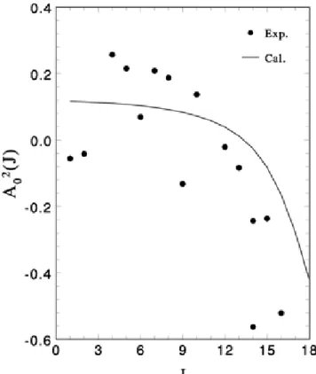
Figure 3.2 shows our calculated results compared with the experimental re-sults of the rotational alignment in the photodesorption of CO from Cr2O3(0001) [9, 10, 11]. The hindrance parameters we used here are V0 = 2000and α = 120◦. It was observed experimentally the quadrupole moment of desorbing CO changes its sign from positive to negative with increasing rotational quantum number J. The-oretically we could reproduce a positive quadrupole moment for small quantum number J and thus corresponds to the helicopter-like desorbing, while a negative quadrupole moment of desorbing CO can be obtained and thus corresponds to the cartwheel-like desorbing for larger quantum number J. This result agrees qualitatively with the experimental observations as can be noted from Fig. 3.2.

To see more profoundly that our calculated results can yield positive values of quadrupole momentum for small angular momentum and negative values for large J states, we examine the expectation value hYJ,m|(3J2z− J2) /J2| YJ,mi in Eq. (3.11). For a specific quantum number J, this expectation value is positive for high |m| values and is negative for low |m| values. In the summation of Eq. (3.11), only the low-lying hindered-rotational states ψ_L,m0 dominate due to

the thermal factor. We calculated the overlapping factors¯¯­YJ,m|ψL,m0®¯¯

2

between the free-rotational states YJ,m and the low-lying hindered-rotational states ψL,m0.

Our results showed that, when J is small, the calculated values of ¯¯­YJ,m|ψL,m0®¯¯

2

for a specific L is larger for ψL,m0 states with larger |m| which correspond to

prefer to the helicopter-like desorption and yield a positive quadrupole moment. On the contrary, when J is larger, the low-lying ψ_L,m0 states correspond smaller

|m| and then negative expectation values hYJ,m|(3J2z− J2) /J2| YJ,mi. Our results also showed that, when J is larger, the calculated values of ¯¯­YJ,m|ψL,m0®¯¯

2 for a specific L is larger for ψ_L,m0 states with smaller |m| which correspond to more

vertically-distributed wavefunctions. This makes the hindered molecule prefer to the cartwheel-like desorption in larger J states and yield a negative quadrupole moment.

3.3

An adsorbed molecule in a strong laser field

Consider now a laser pulse polarizing in z-direction interacts with the hindered molecule. The model Hamiltonian can be written as

H = BL2+ Vhin(θ) + HI, (3.12) where L2 and B are the angular momentum operator and rotational constant. For the vertical absorbed configuration, the surface potential which was proposed by Gadzuk [2, 3] can be written as

Vhin(θ) = ⎧ ⎪ ⎪ ⎨ ⎪ ⎪ ⎩ 0, 0_{≤ θ ≤ α} ∞, α < θ ≤ π , (3.13)

where α is the hindered angle of the conical well. In Eq. (3.12), HI describes the interaction between the dipole moment (permanent and induced) and laser field:

where µ is the dipole moment and ε is the electric field vector of the linearly polarized laser. In the presence of an electric field, the dipole moment can be expressed as [41, 42] µ = µ₀+ 1 2αε + 1 6βε 2 + 1 24γε 3 + ..., (3.15)

where µ0 is the permanent dipole moment, α is the polarizability tensor, and β and γ are the first and second hyperpolarizability tensors. We neglect the higher order terms here, and subsequently the laser-molecule interaction is given by

HI =−µ0E (t) cos θ− 1 2E

2_{(t) ((α}

k− α⊥) cos2θ + α⊥), (3.16)

where the components of the polarizability α_k and α_⊥ are parallel and perpendic-ular to the molecperpendic-ular axis, respectively. The laser field in our consideration is a Gaussian shape centered at the time t0:

E (t) = E0e−

(t_−t0)2

σ2 cos (ωt) , (3.17)

where E0 is the field strength, σ is the pulse duration, and ω is the laser frequency. To solve time-dependent Schrödinger equation, the wavefunction is expressed in terms of a series of eigenfunctions

Ψ(t) =Xcl,m(t) ψl,m(θ, φ) , (3.18)

where cl,m(t) is time-dependent coefficients corresponding to the quantum num-bers (l, m). As can be seen in the above section, the wavefunction for infinite

conical-well model is given by ψ_l,m(θ, φ) = ⎧ ⎪ ⎪ ⎨ ⎪ ⎪ ⎩ Al,mPν|m|l,m(cos θ) exp(imφ) √ 2π , 0 ≤ θ ≤ α 0, α < θ _{≤ π} , (3.19)

where Al,m is the normalization constant and Pν|m|l,m is associated Legendre

func-tion of arbitrary order. After determining the coefficients cl,m(t), the orientation hcos θi and alignment hcos2_θ

i can be carried out immediately.

We choose ICl as our model molecule, whose dipole moment µ = 1.24 Debye, rotational constant B =0.114 cm−1_{, polarizability components α}

k ≈ 18 Å3 and α_{⊥ ≈ 9 Å}3_{. The peak intensity and frequency of laser pulse is about 5 × 10}11 W/cm2 _{and 210 cm}−1_{, respectively. For simplicity (zero-temperature case), the} rotor is assumed in ground state initially, i.e. c0,0(t = 0) = 1. Besides, in order to keep the simulations promising, the highest quantum number for numerical calculations is l = 15, such that the results are convergent and the precision is to the order of 10−7_.

3.4

Results and discussion

The solid lines in the insets of Fig. 3.3 show the dependence of the alignment on hindered angle α. For α = 60◦_{, sinusoidal-like behavior is presented, and the} alignment ranges from 0.63 to 0.91. As the hindered angle increases, the curves become more and more complicated and gradually approach the free rotor limit

can be understood well by studying the populations |cl,m| 2

of low-lying states. In the regime of small hindered angle, there is little chance for electron to populate in higher excited states since the shrinking of the conical-well angle causes the increasing of energy spacings.

One also notes that the populations of a hindered molecule for α = 60◦ _and 120◦_{, shown in Fig. 3.4(a) and (b), mainly compose of l = 0, 1 and 2 states, while} the population of a free rotor is composed of l = 0, 2, 4 states. The underlying physics comes from the reason that ­ψl0,m0|cos2θ| ψl,m

®

is non-zero for all l and l0 _{values in the case of hindered rotation. But it is zero in free rotor limit except} for l = l0 _{or l = l}0_{± 2. The dotted lines in the insets represent the first two main} contributions of the factors P

l6=l0

­

ψl0,m0|cos2θ| ψl,m ®

summed from low-lying states, i.e. the sum of the largest two values of the off-diagonal term­ψ_l0_,m0|cos2θ| ψ_l,m

® . As can be seen, the populations for small hindered angle are mainly distributed on lower states since the main oscillation feature (e.g. the frequency) of the curve (dotted lines) is quite similar to that from whole contributions (solid lines).

Let us now turn our attention to the case of orientation. After applying a short pulse laser, the orientation hcos θi of a hindered molecule (α = 60◦₎ oscil-lates sinusoidally with time as shown in Fig. 3.4(a). The value of hcos θi is always positive because the rotational wavefunction is compressed heavily. As the hin-dered angle α becomes larger, the oscillation frequency also decreases as shown in Fig. 3.4(b). These signatures are quite close to that of the alignment. We

then conclude that even at larger hindered angle (α = 1200_{) the role of hindered} potential still overwhelms the laser pulse, otherwise, the value of hcos θi should not always be positive.

Fig. 3.4(c) represents results of orientations in infinite (V0 =∞) or finite (V0 = 100) conical-well potential for α = 1750_{. Dashed and dotted lines correspond to} V0 = ∞ and 100, respectively. For the case of finite conical-well potential, the wavefunction is expressed in terms of a series of the basis wavefunctions obtained in Refs. [4, 5, 7]. As can be seen, the effect of laser pulse is obvious because negative value appears. Comparing the results with the free orientation [20], the angular distributions for finite well are more isotropic since the wave functions can penetrate into the conical-barrier.

Further analysis shows that components of orientation hcos θi or alignment hcos2_θ

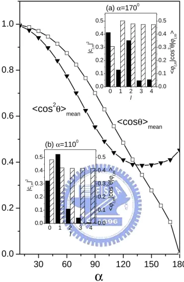
i can be divided into two parts: diagonal and nondiagonal terms. The nondiagonal term represents the variations of these curves such as those in the insets of Fig. 3.3. These variations with time are determined by the phase differ-ence coming from various energy levels. To see the contributions from diagonal terms, we evaluate the time-averaged orientation and alignment. In this case, the nondiagonal values will be averaged out, and only contributions from diagonal terms exit. Fig. 3.5 shows the mean orientation and alignment as a function of hindered angle. As α increases, the mean orientation decreases monotonically

­

ψl,m|cos θ| ψl,m ®

. For a larger angle α, the populations |cl,m| 2

mainly compose of l = 0, 2, 4 states. But the value ­ψ_{l,m|cos θ| ψl,m}® is governed by the selection rule: l = l0 + 1. Thus the net effect is the shrinking of the mean orientation in large angle limit.

Contrary to orientation, the mean alignment shows a quite different feature. The value of hcos2_θ

i first decreases as α increases. However, it reaches a minimum point about for α = 1400_{. From the insets of Fig. 3.5, we know that the values} of ¡­ψ_l,m|cos2_θ

| ψl,m ®¢

do not depend significantly on α. Therefore, the decrease of hcos2θ_{i comes from the decreasing tendency of the population |c}l=1,m|2, while its increasing behavior is caused by other two populations |cl=0,m|

2

and |cl=2,m| 2

. Competition between these two effects results in a minimum point.

Figure 3.2: Quadrupole moments for the desorption of CO from Cr2O3(0001) as function of quantum number J. Filled circles: experimental data points.

0 1 2 3 4 5 6 0.0 0.2 0.4 (c) time [ps] l 0.0 0.2 0.4 (b) time [ps] Populat ion 0.0 0.2 0.4 0.6 0.8 1.0 (a) time [ps] 0 50 100 150 200 250 0.0 0.4 0.8 0 50 100 150 200 250 0.0 0.4 0.8 0 25 50 75 0.0 0.4 0.8

Figure 3.3: The populations of the states (l, m = 0) for different hindered angles: (a) α = 600, (b) α = 1200, (c) α = 1800. The insets show the correspond-ing alignments (solid lines) and the first two main contributions of the factors

P l6=l0 ­ ψ_l0,m0|cos2θ| ψl,m ® (dotted lines).

0 100 200 300 400 500 -0.5 0.0 0.5 0.0 0.5 1.0 0 50 100 150 0.8 0.9 1.0 (c) time [ps] (b) <cos θ > <cos θ > <cos θ > (a)

Figure 3.4: The orientations hcos θi (solid lines) of a hindered molecule confined by infinite conical-well for different hindered angles: (a) α = 600_{, (b) α = 120}0_, (c) α = 1750_{. The dashed and dotted lines in (c) correspond to different potential} barrier height, i.e. V0 =∞ and 100, respectively.

30 60 90 120 150 180 0.0 0.2 0.4 0.6 0.8 1.0 <cosθ>_mean <cos2θ>_mean (b) α=1100 (a) α=1700 < ϕl,m |c o s 2 θ |ϕl,m > < ϕl,m |c o s 2 θ |ϕl,m >

α

Figure 3.5: The mean orientation hcos θimean and alignment hcos2θimean in infi-nite conical-well. The insets show the populations |cl,m|2 (fulled bar) and factors ­

ψl,m|cos2θ| ψl,m ®

(sparse bar). Insets (a) and (b) correspond to α = 1100 and α = 1700_{,respectively.}

CHAPTER 4

COUPLED FREE MOLECULES IN LASER FIELDS

Recently, coupled-rotor- model attracts much interest because some physi-cal properties such as dielectric response may display peculiar behaviors in the presence of dipole-dipole interaction. In some materials, molecules are found to show a free rotation. For example, NH3 groups behave like one-dimensional quantum rotors in certain Hofmann clathrates [25]. In particular, a line broad-ening mechanism is proposed based on rotor-rotor coupling. With the advances of nanotechnology, one can investigate the quantum rotors which are mounted on the surfaces [29, 30, 31]. From the laser spectroscopy, two individual fluo-rescent molecules separated by several nanometers on the surface of an organic crystal can be resolved. The coherent interactions between the dipole moments associated with their optical transitions are found in the quantum optical mea-surements. The strong dipole-dipole coupling produces entangled subradiant and superradiant states in the two molecules system under laser radiation [30].

Many efforts have been devoted to generate entanglement in quantum-optic and atomic systems. Although some studies have been investigated on quantum rotors, these works are limited in the model of kicked tops [43, 44]. In this chapter, we consider a more realistic system. A method is proposed to create entanglement

between two coupled identical polar molecules separated in a distance of tens of nanometers. Both molecules are assumed to be irradiated simultaneously by the laser pulses. It is found that the entanglement induced by the dipole interaction can be affected by controlling the inter-molecule distance, the field strength, and the number of laser pulses. Moreover, the crossover from quantum to classical limit is also discussed by varying the Planck constant.

4.1

Model of two coupled free molecules in a strong laser pulse

Consider now two diatomic polar molecules (e.g. NaI) separated in a dis-tance of R. The molecule system is irradiated by half-cycle pulses. The total Hamiltonian can be written as

H = X j=1,2 ¯ h2 2IL 2 j + Udip+ HI, (4.1) where L2 j and ¯ h2

2I (= B) are the angular momentum operator and rotational con-stant, respectively. Udip is the dipole interaction between two molecules:

Udip =

[µ1· µ2− 3 (µ1· beR) (µ2· beR)]

R3 , (4.2)

where µ1 and µ2 are the dipole moments. The dipole moments of two molecules are assumed, for simplicity, to be identical, i.e. µ1 = µ2 = µ0. The field-molecule coupling HI can thus be expressed as

where θ1 and θ2 are angles between dipole moments and laser field. The laser field is given by E (t, v) = E0f (t) cos (2πvt) ,where E0 is the field strength and v is the frequency. The envelope function f (t) is assumed to be Gaussian shape centered at the time t = t0 with duration σ, i.e. f (t) = e−(t−t0)

2

/σ2

. Traditionally, a half-cycle pulse is a strongly asymmetric monohalf-cycle pulse that consists of two parts: a very short, strong pulse and a much long and weak tail of opposite electrical field. The pulses E (t, v) used in the present work are actually not the exact half-cycle pulses as defined in Ref. [45]. However, practical calculation shows that there is almost no influence on our final result if a long and weak tail is introduced in the pulses E (t, v) = E0f (t) cos (2πvt). Thus, it is reasonable to model a half-cycle pulse by using the function E (t, v) in our calculation. In addition, the field duration is considered to be much shorter than the molecular rotational period in our work. Based on these conditions, an impulsive model can be employed in this case [20, 21]. The time-dependent Schrödinger equation can be solved by expanding the wave function Ψ in terms of a series of field-free spherical harmonic functions Yl,m(θ, φ)as

|Ψi = X

l1,m1;l2,m2

cl1,m1;l2,m2(t)|Yl1,m1(θ1, φ1)i |Yl2,m2(θ2, φ2)i , (4.4)

where (θ1, φ1) and (θ2, φ2)are the coordinates of the first and second molecule re-spectively. The time-dependent coefficients cl1,m1;l2,m2(t) correspond to the

quan-tum numbers (l1, m1; l2, m2)and can be determined by solving Schrödinger equa-tions numerically. In equation (4.4), the inter-molecule separation R is assumed to

be fixed for simplicity, so that the total wavefunction has no spatial dependence. Although the variation of R might be inevitable due to the influence of laser fields or inter-molecule vibrations, however, recent experiments exhibited that the spa-tial resolution in tens of nanometers for two individual molecules hindered on a surface is practically possible [29, 30, 31]. In principle, the free orientation model can be easily generalized to the hindered ones by replacing the spherical harmonic functions with hindered wavefunctions.

4.2

Entanglement of two coupled free molecules

Let us now focus on the entanglement generated in our system. The cou-pled molecules can be expressed as a pure bipartite system. The reduced density operator for the first molecule is defined as

ρ_mol1 = Trmol2|Ψi hΨ| . (4.5)

To study the degree of entanglement, the bases of molecule 1 is transformed to make the reduced density matrix ρmol1 to be diagonal. The entangled state can be represented by a biorthogonal expression with positive real coefficients λlm which can be obtained by diagonalization of density matrix ρmol1. The degree of entanglement for the coupled molecules can then be measured by von Neumann entropy [46, 47]

In our work, NaI molecule in the ground state with dipole moment 9.2 debyes and rotational constant 0.12 cm−1 _{is used. The field strength is 3 × 10}7 _{V/m and the} laser frequency is about 9 × 1011 s−1. The duration and center of the pulse are set equal to 279 fs and 1200 fs. The main feature is that the ratio in magnitude of the positive and negative peak value of the laser pulse is 5 : 1. Unless specified, the parameters of the pulse are fixed throughout the chapter. The crossover from non-entangled case to entangled one is studied based on the initial condition:

c0,0;0,0(t = 0) = 1.

4.3

Results and discussion

After the coefficients cl1,m1;l2,m2(t) are determined, the orientations hcos θ1i

and hcos θ2i can be evaluated immediately. Fig. 4.1 shows the orientations of the first and second molecules after a single laser pulse is applied on both molecules. For R = 3 × 10−8 m, the behavior of the first molecule is quite close to that of a free rotor [20]. This is not surprising because the dipole interaction is weak for this molecule separation. However, as two molecules get close enough (Fig. 4.1(b)), both molecules orient disorderly, and the periodic behavior disappears. This is because the dipole interaction is increased as the distance between the molecules is decreased, and the energy exchange between two molecules becomes more frequently. The regular orientation caused by the laser pulse is inhibited by the mutual interaction.

The populations of some low-energy levels are shown in the lower panels of Fig. 4.1(a) and (b). The solid, dashed, and dotted lines represent the populations of the states (1,0;0,0), (1,0;1,0), and (2,0;1,0), respectively. These states show different degrees of periodic behavior at different distances. However, the populations of some higher excited states, for example the (3,0;1,0) state in the inset of Fig. 4.1(b), display different degrees of irregularity. This manifests a fact that the nonlinear effect, caused by the reduction of R, does not affect the regularity of the low-lying states, and the origin of the irregularity is caused by the higher excited states.

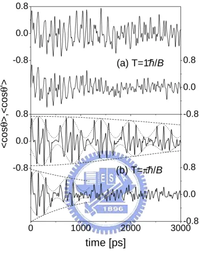
Consider now the molecules are irradiated by a series of laser pulses periodi-cally. As shown in Fig. 4.2(a), if the period of the applied periodically laser pulse T is equal to ¯h/B , then both molecules behave disorderly no matter how the distance R is varied. The chaotic behavior of the molecules can be ascribed to the well-known ”kicked-rotor”problem. However, a series of regular-like orientations marked by dotted and dashed lines are present in Fig. 4.2(b) if T is equal to π¯h/B. For a free rotor under a single kick, this interesting phenomenon comes from the situation as the magnitude of the orientation returns to its initial con-dition (hcos θi = 0) after a certain period T [20]. Therefore, for two molecules in weak interaction limit (R = 3 × 10−8 _{m), the wavepacket-like orientation is} similar to that of a single free rotor under the same laser period. The difference

the dipole force can generate some accidental phases to perturb the regularity of the coupled system. The lower panel of Fig 4.2(b) exhibits that the suppression of the regularity is quicker if the dipole force is stronger.

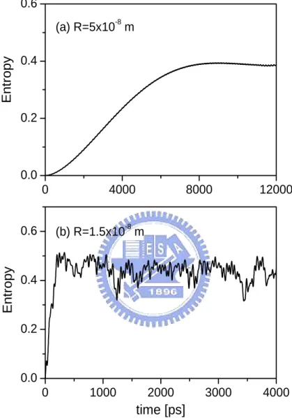
Fig. 4.3 shows the time-dependent entropy after one pulse passes through this system. For inter-distance R = 5 × 10−8 _{m, the entropy increases slowly} from zero. For R = 1.5 × 10−8 _{m, on the contrary, the entropy grows rapidly} with the increasing of time because the dipole force is stronger. Notes that the entropy only varies within a finite range at long time regime. This indicates that the systems reaches a dynamic equilibrium state even though the dipole force is still present.

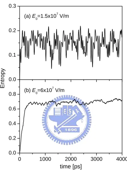
Fig. 4.4(a) illustrates the variations of the entropy with respect to different field strengths of the applied laser pulse as R is set equal to 1.5 × 10−8 _{m. For} the field strength E0 = 1.5× 107 V/m, an irregular-like behavior of the entropy is obtained, and its value is not large enough for quantum information processing. However, Fig. 4.4(b) shows that the degree of entanglement can be enhanced if one increases the field strength. This can be understood well by studying the relationship between the dipolar interaction and the field strength. If the effect of dipole interaction overwhelms the laser field, most of the populations are distrib-uted on the low-lying states. In this case, the entropy from Schmidt decomposition is certainly small as shown in Fig. 4.4(a). On the other hand, if the field strength plays a dominant role, the distribution of molecular states covers a wider range

and the entropy is enhanced in this limit.

Next we detune the frequencies of the laser fields to study the behavior of entanglement. Figure 4.5 illustrates the time evolution of the entropy with dif-ferent ratios in magnitude of the positive and negative peak value of the laser pulse as R is set equal to 1.5 × 10−8 _{m. The laser frequency is tuned to change} the ratio as shown in the inset by fixing other parameters. For the case of ratio 9 : 1, an irregular-like behavior is obtained with time-averaged value 0.51. If the ratio is set equal to 1 : 1, the entanglement shows a nearly periodic behavior with small averaged entropy. This result is very similar to the limiting case without laser, and indicates that the entanglement depends sensitively on the ratio of the laser pulse, i.e. the excitation is suppressed under the condition of 1 : 1 ratio. Meanwhile, the dipole force only establishes periodic-like entropy.

Let us consider the first ten most contributive coefficients λl,m. The λl,m are re-arranged and denoted as λp with p = 1, 2, 3.... For example, λ1 is the most contributive coefficient. The insets of Fig. 4.5 show the ten coefficients (λp) at short and long time regimes. In the case of the ratio 9 : 1 , the eigenvalue λ1 dominates the contributions at short time regime(t = 50 ps). However, the contributions are distributed more averagely between different levels as t = 800 ps regime. This means the system is in some sort of dynamic equilibrium in long time limit, and entropy saturates to certain value. On the contrary, λ1 always

ratio 1 : 1 as shown in the lower inset of Fig. 4.5. From statistical point of view, this somehow explains the suppressed and regular behaviors of the entanglement (entropy).

Figure 4.6 shows the time evolutions of the populations of the eigenstates for different ratio of pulse shapes. For 1 : 1 ratio, the pulse hardly excites the rotors from the initial energy level (0, 0; 0, 0). Therefore, (0, 0; 0, 0) is still the mostly populated level (the population value is nearly close to 1 ) as shown in the lower panel of Fig. 4.6 while the pulse passes through. Similar to the ground state, the populations of the higher levels (the inset of Fig. 4.6) also show the periodic behavior. The periodic behavior is ascribed to the dipole interaction. Since the small fluctuation of the population is dominated by the dipole interaction in the case of symmetrical pulses. The magnitudes of the periodic fluctuations in higher level populations are rather small with the periodic evolution of the entropy. On the other hand, for 9 : 1 ratio the populations of the higher states show different degrees of irregularity as shown in the upper panel of Fig. 4.6. This is because a single asymmetrical pulse can generate high populations in the excited states [20], i.e. a larger angle orientation. The larger angle orientation can cause a largely fluctuated dipole interaction between the molecules. For this situation, energy transfer by means of (mediated) dipole interaction generates the irregular evolutions of the higher excited states which result in a randomly time-varying entropy.

We further study the entropy for different separation and dipole moment in Fig. 4.7. The ratio is set equal to 9 : 1. If the separation is smaller (0.8 R), the entropy grows faster. On the contrary, the entropy evolves slower for the case of larger separation. This means that the system needs much more time to approach the dynamic equilibrium. We also study the time evolution of entropy by changing the dipole moment. Our result shows that a similar behavior of the entropy exhibits, i.e. the strength of dipole interaction governs the behavior of evolution.

By adjusting the laser parameters, one can vary the degree of the entangle-ment. Figure 4.8 illustrates the time evolution of the entropy under single pulse or double pulses with ratio 5 : 1. As can be seen, an irregular behavior of the entropy is obtained, but their averaged values are different. For single kick, the populations are first dominated by this laser pulse. Then, the dipole interaction plays a key role to raise the entanglement in the system. In the case of double pulses the finite populations is created by first pulse. As the second laser pulse passes through, the populations will be redistributed to a wider range. Since the populations are distributed more averagely in this case, the entropy is certainly larger as shown by the solid line in Fig. 4.8. One can notes that the enhancement of entropy is achieved by applying the second laser pulse. Consider the case that time separation between these two pulses is set to be 5 times the center of the

tuned to obtain different degree of entropy. Another way to control the degree of entanglement in this system is to change the positive and negative ratios of the laser pulse. Inset of Fig. 4.8 shows the time-averaged entropy with respect to different ratios. We find that the entropy is more enhanced as the ratio is larger. This means that the highly asymmetric laser pulse can generate larger entropy under the same field strength.

To study the crossover behavior from quantum to classical limit in this system, one can tune the fundamental Planck constant ¯h0. Figure 4.9 shows the time for entropy first exceeds the time-averaged value (arrow in the inset) versus the different factor of Planck constant ¯h0. As shown, the time grows rapidly with the decreasing of the Planck constant ¯h0. The inset in Fig. 4.9 shows a slowly increasing of entropy with the evolution of time for ¯h0 = 0.01¯h. Comparing this with the result for ¯h0 = ¯h, the ratio of the two times is roughly 100 : 1. This means that the entropy evolves slowly, and the system needs a longer time to approach dynamical equilibrium for a small ¯h0. As expected, the time for classical limit (¯h0 _{→ 0) goes to infinity, satisfying that no entanglement exists between classical} objects.

For a more realistic molecular system, one can extend our model to hindered-rotor system. The hindered hindered-rotor means that the polar diatomic molecule is adsorbed on the surface with the confinement of surface potential. In other words, one reasonably considers that two coupled polar molecules are adsorbed on the

surface with the dipole interaction. Comparing hindered rotor with free one, the rotation of a hindered rotor is similar to that for the free one, but the degree of orientation is different. This is because that the surface potential confines the rotation. Although this confinement may affect the property of the system, according to our work in chapter 3, a free rotor and hindered rotor actually show the same physics. In particular, a hindered rotor can be transformed into a free one by changing the parameters of surface potential.

0 1000 2000 3000 0.0 0.4 0.0 0.8 0.0 0.4 -0.8 0.0 0.8 time [ps] (b) R=1.5x10-8 m (a) R=3x10-8 m |c l 1 ,m 1 ;l2 ,m 2 (t )| 2 |c l 1 ,m 1 ;l2 ,m 2 (t )| 2 <cos θ > (<c o s θ '>) <cos θ > (<c o s θ '>) 0 2000 4000 0.00 0.02 0 2000 4000 0.00 0.02

Figure 4.1: Upper panels of Fig. 4.1(a) and (b) show the orientations of the two molecules at different distances. Lower panels: The populations of the states (l1, m1; l2, m2)=(1, 0; 0, 0) (solid lines), (2, 0; 1, 0) (dotted lines), (1, 0; 1, 0) (dashed lines). The insets in (a) and (b) represent the population of state (3, 0; 1, 0) .

0 1000 2000 3000-0.8 0.0 0.8 -0.8 0.0 0.8 -0.8 0.0 0.8 -0.8 0.0 0.8 (b) T=_πh/B

time [ps]

Figure 4.2: The orientations of the first and second molecules under periodic laser pulses with the periods T= (a) 1¯h/B, (b) π¯h/B ps. The upper and lower panels of (a) and (b) correspond to the distances R = 3 × 10−8 _{and 2 × 10}−8 _m, respectively.

0 1000 2000 3000 4000 0.0 0.2 0.4 0.6 0 4000 8000 12000 0.0 0.2 0.4 0.6 (b) R=1.5x10-8 m Ent ropy Ent ropy time [ps] (a) R=5x10-8 m

Figure 4.3: Time evolution of the entropy after applying single laser pulse for (a) R = 5 _{× 10}−8 _{m and (b) R = 1.5 × 10}−8 _m.

0 1000 2000 3000 4000 0.0 0.2 0.4 0.6 0.8 0.0 0.1 0.2 0.3 (b) E 0=6x10 7 V/m Ent ropy time [ps] (a) E 0=1.5x10 7 V/m

Figure 4.4: Time evolution of the entropy for inter-molecule separation R = 1.5 × 10−8 _{m. The degree of entanglement can be enhanced if one increases the field} strength.

0 200 400 600 800 1000 0.0 0.1 0.2 0.3 0.4 0.5 0.6 λ p p

time [ps]

Figure 4.5: Time evolution of the entropy after applying single laser pulse for different ratios in magnitudes of the positive and negative peak value of the laser pulse. The graphs show the irregular (periodic) behavior for ratio 9 : 1 (1 : 1). The inset : the first ten contributive eigenvalues λp at short time (t = 50 ps) and long time (t = 800 ps).

0 200 400 600 800 1000 0.0 0.2 0.4 0.6 0.8 1.0 0.0 0.1 0.2 0.3 ratio=1:1 time [ps] ratio=9:1 |cl 1 ,m 1 ;l2 ,m 2 (t )| 2 |cl 1 ,m 1 ;l2 ,m 2 (t )| 2 0 500 1000 0.00 0.02 0.04 0.06

Figure 4.6: Populations of the states (l1, m1; l2, m2) for different ratios. Upper panel : (1, 0; 0, 0) (dashed line), (1, 0; 1, 0) (solid line), (2, 0; 1, 0) (dotted line). Lower panel : (0, 0; 0, 0) (dashed line), (1, 0; 1, 0) (solid line), (1, 1; 1, 1) (dot-ted line). The inset in the lower panel is the enlarged figure showing the states (1, 0; 1, 0) (solid line), (1, 1; 1, 1) (dotted line), respectively.

0 200 400 600 800 1000 0.0 0.1 0.2 0.3 0.4 0.5 0.6 0.0 0.1 0.2 0.3 0.4 0.5 0.6 1.2 µ µ 0.8 µ time [ps] (b) (a) 0.8 R R 1.2 R E nt ropy E nt ropy

Figure 4.7: Time evolution of the entropy for different separation and dipole moment under single pulse (ratio 9 : 1). The dotted curve shows the case of R = 1.5_{× 10}−8 _{m and µ = 9.2 D. The dashed and solid curves correspond to (a)} 0.8 R and 1.2 R, or (b) 1.2 µ and 0.8 µ, respectively.

0 200 400 600 800 1000 0.0 0.1 0.2 0.3 0.4 0.5 0.6 0.7 0.8 0.9 ratio E nt ropy mean

time [ps]

Figure 4.8: Time evolution of the entropy for fixed ratio 5 : 1 under single pulse (dashed line) and double pulses (solid line). Time separation (tapp) between two pulses is set to be 5 times the center of the laser peak. The inset : Dependence of the time-averaged entropy on the pulse shape for inter-molecule separation R = 1.5 _{× 10}−8 _m.

0.0 0.2 0.4 0.6 0.8 1.0 0 5000 10000 15000 20000 25000 30000 35000 40000 45000 Ti me [p s] Planck constant h' [h] time [ps] E n tr opy 0.01h h 0 10000 20000 30000 40000 0.0 0.1 0.2 0.3 0.4 0.5 0.6 h'=0.01h

Figure 4.9: The time with respect to different Planck constant ¯h0 for fixed field strength E0 = 3× 107 V/m and inter-molecule separation R = 1.5 × 10−8 m. The time is defined as the first time in entropy that exceeds the time-averaged value (the arrow in the inset). The inset : the time-averaged value (dotted line), and time evolution of the entropy for ¯h0 = 0.01¯h (solid line).

CHAPTER 5

COUPLED ADSORBED MOLECULES IN LASER

FIELDS

In the complex surface systems, adsorbed molecules may not be isolated. Several studies have shown that interesting behavior can occur due to the existence of dipole-dipole interaction [24, 25, 26, 27, 28]. In addition, since the investigations on entangled behavior of two coupled rotors are limited in the model of kicked tops [43, 44], this inspires us to study the dynamical entanglement of adsorbed molecules. According to our study in chapter 3, it is found that the orientations of free coupled rotors somehow reflect the entropy of the system and thus relate to the measurement of entanglement. Since the entanglement measurement is one of the fundamental important issues in quantum information research, the study of the entanglement and its measurement becomes an interesting problem. Moreover, from the experimental point of view, it is still not clear how to keep two free rotors with fixed distance. Therefore, this makes it more interesting to consider a more realistic system and discuss the corresponding entanglement dynamics.

pulse, the hindered rotor shows periodic behavior. Different signatures between the finite-conical-well and infinite-conical-well model on orientations are pointed out. Besides, the amplitudes of the oscillations are varied by applying different widths of the pulse. Furthermore, we also consider two coupled identical polar molecules adsorbed on the surface with the dipole-dipole interaction and a si-multaneously ultra-short laser pulse shined upon them. It is found that both the entanglement (the von Neumann entropy) and orientation show interesting behaviors.

5.1

Single adsorbed molecule in a strong laser pulse

Consider now a dipolar molecule (e.g. NaI) adsorbed on the surface. The rotation of the molecule is confined by the surface potential as shown in Fig. 5.1. An off-resonant laser field polarized in z-direction interacts with the hindered rotor. Because the laser frequency is much lower than the frequencies of the lowest vibrational and electronic transition, only the rotational excitations can occur in our model. The excitations can be viewed as two photon transitions between two different rotational states through a high intermediate virtual state [18]. The Hamiltonian without the field-molecule interaction can be written as

H0 = BJ2+ Vhin(θ, φ), (5.1)

where B and J2 are rotational constant and angular momentum. Vhin denotes the surface potential and confines the rotation of adsorbed molecule. For simplicity,

the infinite-conical-well model Vhin(θ, φ) is considered here. According to the previous studies, its dependence on φ is weaker than that on θ [32, 33, 34]. We reasonably assume that the surface potential is independent of φ. Therefore, in the vertical adsorbed configuration, the surface potential can be written as [3]

Vhin(θ) = ⎧ ⎪ ⎪ ⎨ ⎪ ⎪ ⎩ 0, 0≤ θ ≤ α ∞, α < θ ≤ π , (5.2)

where α is the hindering angle of the conical well.

The Hamiltonian concerning the field-molecule interaction can be written as Hd =−µE (t) cos θ, (5.3) Hind =− 1 2E 2_{(t) ((α} k− α⊥) cos2θ + α⊥). (5.4) The first term Hddescribes a permanent dipole moment µ coupling with an exter-nal field, and θ is the angle between the molecular axis and the field. In this work we choose a Gaussian pulse for our calculation, i.e. E (t) = E0e−(t−t0)

2_/σ2

cos (2πνt) , where E0 is the field strength and ν is the laser frequency. The pulse is centered at the time t0, and σ is the pulse duration. The second term Hind is a higher order interaction, in which the external field couples with the induced molecular polarization. The component of the polarizability α_k (α⊥)is parallel (perpendicu-lar) to the molecular axis. According to our parameters, the field-dipole-moment interaction Hd is much greater than that of the field-induced-dipole-moment in-teraction Hind in our model. This is because the strength of electric field used