國 立 交 通 大 學
環 境 工 程 研 究 所
碩 士 論 文
滲漏含水層考慮彎曲效應之地下水流半解析解
Semi-Analytical Solution of Groundwater Flow in a Leaky
Confined Aquifer under Bending Effect
研 究 生:游 佳 琪
指 導 教 授:葉 弘 德 教授
滲漏含水層考慮彎曲效應之地下水流半解析解
Semi-Analytical Solution of Groundwater Flow in a
Leaky Confined Aquifer under Bending Effect
研 究 生:游佳琪
Student:Chia-Chi Yu
指導教授:葉弘德
Advisor:Hund-Der Yeh
國 立 交 通 大 學
環 境 工 程 研 究 所
碩 士 論 文
A ThesisSubmitted to Institute of Environmental Engineering College of Engineering
National Chiao Tung University in Partial Fulfillment of the Requirements
for the Degree of Master of Science in Environmental Engineering June, 2012 Hsinchu, Taiwan
中 華 民 國 一 ○ 一 年 六 月
滲漏含水層考慮彎曲效應之地下水流半解析解
研究生:游佳琪
指導教授:葉弘德
國立交通大學環境工程研究所
摘 要
傳統地下水理論假設含水層總應力為一定值,且忽略受壓含水層在抽水時所 伴隨產生的力學行為,但實際抽水時,水層結構可能會像平板一樣彎曲。本研究 目的為探討定流量抽水下,推導滲漏受壓含水層受到彎曲效應影響所產生洩降分 佈的半解析解。本研究利用所發展出的半解析解,探討滲漏受壓含水層系統在定 抽水率下,洩降分佈受到彎曲及滲漏效應的影響。藉由建立數學模式,以描述滲 漏受壓含水層系統承受滯水層中彎曲效應影響的洩降分佈。此模式包括三個耦合 的控制方程式,分別是描述受壓水層暫態洩降分佈方程式、滲漏水層暫態洩降分 佈方程式、及基於板殼理論所描述水層彎曲效應的方程式;接著,針對此三個方 程式,應用拉普拉斯(Laplace)和漢可爾(Hankel)轉換方法求得模式的半解析 解,最後,使用修正 Crump 方法進行數值逆轉推求時間域的結果。此新解在忽 略彎曲或滲漏效應下,可分別簡化至拉普拉斯域的 Hantush (1960) 解和時間域的 Wang et al. (2004) 解。本研究利用所推得的解作分析,顯示抽水試驗初期含水層 洩降受到彎曲效應的影響,而試驗晚期則受到含水層滲漏因子的影響較為明顯。 敏感度分析結果顯示,含水層壓縮性只在試驗初期敏感,造成含水層釋放出的水 量較傳統地下水理論估計值小。因含水層洩降分佈在試驗晚期對滯水層水力傳導 係數較具敏感度,導致相較於無滲漏受壓含水層具有較小的含水層洩降分佈。此 外,洩降對含水層的厚度及水力傳導係數具有最高的敏感度。Semi-Analytical Solution of Groundwater flow in a
Leaky Confined Aquifer under Bending Effect
Student:Chia-Chi Yu
Advisor:Hund-Der Yeh
Institute of Environmental Engineering
National Chiao Tung University
ABSTRACT
Traditionally, the groundwater flow induced by pumping often assumes that the total stress of aquifer maintains constant all the time and the aquitard mechanical behavior is negligible. The formation of the aquifer system may actually bend like a plate when subject to pumping. This study aims at developing a new semi-analytical model for investigating the impacts of aquitard bending and leakage rate on the drawdown of the confined aquifer due to a constant-rate pumping in a leaky confined aquifer (LCA) system. A mathematical model is first build for delineating the LCA drawdown distribution subject to bending effect emerged in the confining unit. This model contains three governing equations, delineating the transient behavior of
displacement based on a thin plate theory of small-deflection in response to aquitard bending. The semi-analytical solution is found by employing the methods of the Laplace transform and Hankel transform. The corresponding time-domain result of the derived solution is established by applying the modified Crump method. Without considering the bending effect, this new solution can reduce to the Hantush solution in Laplace domain (Hantush, M.S., 1960. Modification of the theory of leaky aquifers. Journal of Geophysical Research 65(11), 3713-3725). On the other hand, this solution reduces to the Wang et al. solution (Wang, X.S., Chen, C.X., Jiao, J.J., 2004. Modified Theis equation by considering the bending effect of the confining unit. Advances in Water Resources 27(10), 981-990.) in time domain when neglecting the leakage effect. The results predicted from the present solution show that the aquifer drawdown will be influenced by the bending effect at early time and the leakage effect at late time. The results of sensitivity analysis indicate that the skeleton compression of the aquifer is sensitive only at early time, causing less amount of water released from pumped aquifer than that predicted by the traditional groundwater theory. The aquifer drawdown is more sensitive to aquitard’s hydraulic conductivity at late time, leading smaller drawdown than non-leaky one. Additionally, both the hydraulic conductivity and thickness of the aquifer are the most sensitive parameters to the predicted drawdown.
Keywords: groundwater; constant-rate pumping; leaky confined aquifer (LCA);
誌 謝
感謝指導老師葉弘德教授讓我在研究路途上更加順遂,其次,感謝萬能科技 大學楊紹洋教授、中央大學葉高次教授與陳瑞昇教授,於口試中提出深入見解與 建議,令本篇論文更顯完整。 感謝雅琪、彥如、珖儀、璟勝、佩蓉、昭志等學長姐,韻如、家豪兩位同窗, 以及芷萱、欣慈、翊岷等學弟妹,有你們的陪伴讓我的研究生活更添風采。另外 特別感謝紹洋學長不僅於研究上給予諸多幫助與指導,更對於生活上的經驗分享 不予保留,使本論文得以順利完成。 在此特別感謝蔡春進教授讓我的人生觀成長許多,並且磨練報告書寫技巧, 豐富了我的成長歷程。同時感謝俊男、技恩、芸伊、紹銘、毅弘、栢森、怡伶等 學長姐,能駿、盧緯、盈禎與香茹四位同窗,謝謝你們對我不離不棄以及諸多鼓 勵。感謝環工所諸位師長、全體同學因為有你們在讓我留下美好的回憶。感謝我 的好友團,努力當個優質垃圾桶,對於任何傾倒下的垃圾都一一吞下。 最後,將本論文獻給我的家人,感謝你們長久以來的支持讓我有機會完成碩 士學歷,由衷的感謝。 佳琪 謹誌於 交通大學環工館 中華民國一○一年六月TABLE OF CONTENTS
摘要……….. I
ABSTRACT………. II
誌謝……….. V
TABLE OF CONTENTS………. VII LIST OF TABLE………... VIII LIST OF FIGURES……….. IX NOTATION………. X CHAPTER 1 INTRODUCTION………. 1 1.1 Background……… 1 1.2 Literature Review………... 2
1.2.1 Pumping drawdown in aquifer systems ………..
2
1.2.2 The thin plate theory on small displacement………….……….
7 1.3 Objectives……….. 8 CHAPTER 2 METHODS……… 10 2.1 Mathematical Model………..……… 11 2.1.1 Aquitard………...………. 12
2.1.2 Vertical downward displacement…….……….
13
2.2 Semi-Analytical Solutions……….
2.2.1 Aquitard flow………
15
2.2.2 Drawdown and vertical downward displacement……….
16
CHAPTER 3 SPECIAL CASES………..
18
3.1 Neglecting bending effect………..
18
3.2 Neglecting the leakage effect……….
19
CHAPTER 4 RESULTS AND DISCUSSION………
20
4.1 Case study: A hypothetical aquifer system………
20
4.2 Analysis based on dimensionless parameters..……….
22 4.3 Sensitivity analysis……… 23 CHAPTER 5 CONCLUTIONS….……….. 26 REFERENCES………...……….. 28 APPENDIX A: DERIVATION OF THE LAPLACE-DOMAIN SOLUTION TO
EQUATIONS (27) AND (28)
LIST OF TABLE
LIST OF FIGURES
Figure 1. Idealized representation of a leaky confined aquifer subject to pumping at a
fully penetrating well.……….. 36 Figure 2. The time-drawdown curves for r = 5 m and 10 m (a) at small time (b) at large
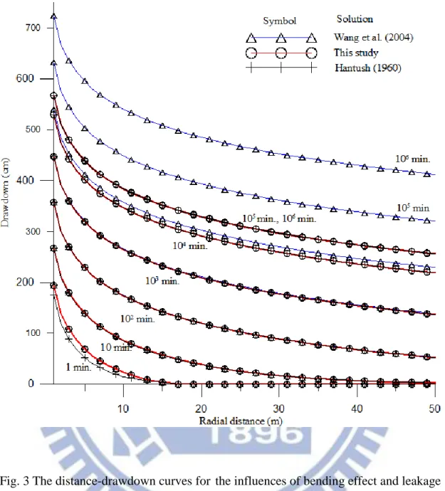
time………. 37 Figure 3.
The distance-drawdown curves for the influences of bending effect and leakage effect………...………...
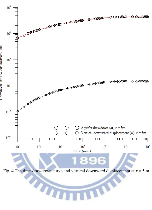
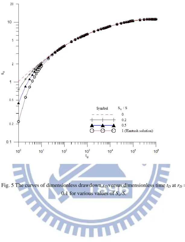
39 Figure 4. The time-drawdown curve and vertical downward displacement at r = 5 m……. 40 Figure 5. The curves of dimensionless drawdown sD versus dimensionless time tD at rD =
0.1 for various values of Sw/S……… 41
Figure 6. Plots of the time-drawdown curve and the normalized sensitivities of the
NOTATION
The following symbols are used in this thesis: b : Aquifer thickness [L]
b' : Aquitard thickness [L]
c : Sm D /w [L4]
D : Flexural rigidity of the aquitard [N.L]
E : Young’s modulus of the aquitard [N/L2]
J0(‧) : Bessel function of first kind of order zero
K' : Hydraulic conductivity of the aquitard [L/t]
n : Porosity of the aquifer
p : Laplace variable
Pz : Lateral pressure [N/m2]
ql : Leakage rate of the aquitard from the centerline of the pumping well [L/t]
Q : Pumping flow rate[L3/t]
r : Radial distance [L]
T : Transmissivity of the aquifer [L2/t]
s : Aquifer drawdown [L]
~
s : Aquifer drawdown in Laplace domain [L]
'
~
s : Aquitard drawdown in Laplace domain [L] s′ : Aquitard drawdown [L]
S : Storage coefficient of the aquifer
S' : Storage coefficient of the aquitard
Sw : Storage coefficient of water expansion
t : Time from the start of the test [t] ν : Poisson’s ratio of the aquitard
w : Vertical downward displacement [L]
z : Vertical distance from the bottom of impermeable layer [L]
α : Compressibility of aquifer matrix [L2/N]
β : Hankel transform parameter
βw : Compressibility of water [L2/N]
) (
: Tβ2(1+cβ4)/(S+Sw cβ4)
w : Specific weight of water [N/L3]
Δp : pore pressure change [N/L2] Δσ : Total stress change [N/L2] Δσ′ : Effective stress variation [N/L2]
η : pS'/(b'K')
CHAPTER 1 INTRODUCTION
1.1 Background
Hantush (1960) presented a Laplace-domain solution of transient drawdown in a leaky confined aquifer (LCA) called as the Hantush solution. His solution was obtained under the assumptions that (1) water was pumped at a constant-flux rate from a fully penetrating well; (2) the aquifer formation was isotropic and homogenous; (3) the leakage rate from the aquitard was proportional to the drawdown at any point; (4) the storages in both the aquitard and aquifer were considered; and (5) the hydraulic head in the layer supplying leakage rate was constant. The Hantush solution was obtained by utilizing the Hankel and Laplace transforms with corresponding boundary conditions.
In the past, the conventional groundwater theory generally assumed the total stress of the aquifer as a constant value and ignored the mechanical behavior in confining unit when the aquifer was subject to pumping. In reality, most geologic formations have rigidity and the aquifer formation may bend like a plate during pumping. Therefore, the amount of water released from aquifer system might differ from the estimation by the traditional groundwater theory. The study of aquifer drawdown and downward vertical displacement provides an important framework for
understanding the drawdown distribution in a LCA system with considering both the bending effect and leakage effect.
1.2 Literature Review
1.2.1 Pumping drawdown in aquifer systems
In the past, there were many studies focusing on the prediction of drawdown distribution in a confined aquifer system. For instance, Denis and Motz (1988) developed a solution for both transient and steady-state drawdowns in a coupled aquifer system. Their solution included the effects of water storage in confining unit and the evapotranspiration (ET) on drawdown distribution. The result showed that the increase in the ET rate caused less pumping time in reaching its steady-state condition. In other words, the increase in confining unit storage made the time to approach its steady-state condition longer, and delayed the drawdown response time, especially within the un-pumping aquifer. Hunt and Scott (2005) pointed out the major difference among three solutions of Theis and Branch (1935), Hantush and Jacob (1955), and Boulton (1954; 1963) for transient flow toward the pumping well, and a new solution was applied to the Boulton solution for free-surface drawdown in the top layer. Note there were two restrictions in their study. One was that the largest transmissivity of any un-pumped layer should not overtake about 5 % to the transmissivity of pumped layer. The other was that the elastic storage of any
un-pumped layer must be less than the specific yield of the top unconfined layer. Based on force balance and transient flow equations, Yeh et al. (1996) developed a three-dimensional Galerkin finite element model for simulating the land displacements due to pumping. Li (2007) presented an analytic solution, by utilizing the velocity and displacement to delineate the aquifer horizontal movement. Additionally, the displacement was induced by well extraction or injection in a LCA system. The result indicated that the vertical water flow was a critical factor for the aquifer radial movement and the radial flow velocity was much more responsive than the aquifer displacement to the vertical flow. Wen et al. (2008) introduced drawdown solutions for non-Darcian flow toward the pumping well in an aquifer-aquitard system with considering the impacts of the wellbore storage and leakage. Through sensitivity analysis, they demonstrated that the leakage effect on drawdown distribution was significant only in late pumping period and the effect of wellbore storage was at early pumping time. In addition, the results of non-Darcian flow compared to Darcian flow showed a larger aquifer drawdown at early pumping time and smaller at late time. Yang and Yeh (2009) provided a mathematical model in a two-zone LCA and developed a transient solution in Laplace domain. Their mathematical model accounted for the influence of skin zone, finite radius well, and aquitard storage. The aquifer drawdown of considering the effects of skin zone and aquitard leakage was
larger than that neglecting those two effects. The leakage effect on drawdown distribution was obvious at late pumping time. Furthermore, a smaller hydraulic conductivity and/or larger thickness of the aquitard led a larger aquifer drawdown. The results of sensitivity analysis showed that the influence of negative skin zone was larger than that of positive skin zone on aquifer drawdown, and the impact of finite radius and aquitard storage on the drawdown was merely significant in the early pumping period.
Zhan and Bian (2006) presented analytical/semi-analytical solutions for constant-flux and constant-drawdown pimping tests in a LCA with a fully penetrating vertical well to predict the leakage rate and volume. They generalized the solutions to finite-size aquifers with lateral impermeable boundaries, which might be practical for managing the multi-layered aquifers. Hunt and Scott (2007) developed an approximate solution to describe water flow toward the pumping well in an aquifer-aquitard-aquifer system. They improved the previous studies of Hemker and Maas (1987) and made the solution much easier, efficient and able to investigate the constraints on approximate solution and physical behavior in the multi-layered aquifer systems. The results indicated that the horizontal flow of aquitard was negligible when both the transmissivity and storage of aquitard were less than 10 % of those the pumped aquifer. Li and Neuman (2007) provided a semi-analytical solution in a
five-layered aquifer system and evaluated the time-domain results through a numerical inversion algorithm. Their results of the solution indicated that the influence of pumping on the drawdown may spread across all five layers during a sufficiently long pumping duration.
Sekhar et al. (1994) developed a numerical model for estimating the parameter of anisotropic leaky aquifer system with unknown principal axes. Their numerical model could addtionally operate under limit data (i.e., only three wells and two pumping test data). The goverening parameters were eatimated by a sensitivity analysis technique. Forthermore, the sensitivity coefficients were assessed based on a modified parameter perturbation techique. Hu and Chen (2008) compared the difference of the analytical and numerical models for transient flow to the pumping well in a confined-unconfined aquifer system. The analytical results indicated that the drawdowns predicted by Chen’s model (Chen, 1974; 1983) were more reasonable than those obtained from Moench and Prickett’s model (Moench and Prickett, 1972) except as the radial distance or aquifer thickness was large. Barua and Bora (2010) obtained a steady/quasi-steady model for a partially penetrating well with a finite skin thickness in a confined aquifer. With pumping test data, the model could determine the skin thickness and the hydraulic conductivities of the skin and formation zones in an artesian aquifer. Previous studies of the analytical and numerical solutions were
mostly based on several assumptions when making the drawdown predictions. On the contrary, the Barua and Bora model (2010) considered various effects (i.e., partially penetrating well, finite skin thickness, bottom flow, and finite horizontal and lateral aquifer flow system) and the model might be more suitable to describe the field tests. Various types of effect on the drawdown distribution in the aquifer system had been investigated by past studies. For instance, the Noordbergum effect and bending effect had been considered to explore their influence on pumping drawdown in an aquifer system. The noordbergum effect (Kim and Parizek, 1997) was produced due to the difference of poroelastic response to hydraulic pumping stress in an aquifer system. Kim and Parizek (1997) applied a linear poroelasticity theory to compare the difference caused by the Noordbergum effect in the aquifer-aquitard-aquifer system and the single-layered aquifer system. They indicated that the Noordbergum effect significantly influenced the drawdown distribution in the early pumping period. Wang et al. (2004) applied the thin plate theory on small deflection to the Theis and Branch equation (1935) and derived an analytical solution describing the aquifer drawdown distribution. The results indicated that the aquifer drawdown under bending effect was larger than that predicted by the Theis and Branch solution (1935), and the difference was obvious near the pumping well at early time. According to field test data, the aquifer drawdown was dramatically affected by the bending effect as water was
pumped from a high compressible aquifer layer.
1.2.2 The thin plate theory on small displacement
The mathematics of Biot’s theory or poroelastic solid theory is much more complicated than the thin plate theory in modeling. The thin plate theory on small displacement is therefore applied to describe the mechanical behavior of a pumped LCA system. A thin plate is defined as the thickness or length of prismatic member (e.g., cylinder) is relatively small compared with the dimensions in the middle surface of the plate. The terminology of small-deflection means that the lateral displacement of the plate in the vertical direction is smaller than a half of the plate thickness (Boresi et al., 1993).
As considering small deflections, the corrdinate axes in the deformed and un-deformed states have a negligible difference; therefore, this study excludes the problem of axes rotation. According to the Kirchoff assumption (Boresi et al., 1993), the straight-line normal to the un-deformed middle surface remains normal to the deformed middle surface. Boresi et al. (1993) combined the strain-displacement relations on small displacement with the Kirchoff assumption for linear elastic isotropic materials to produce the governing equation describing the bending of the thin plate.
1.3 Objectives
The total stress of the aquifer system is generally assumed to be constant in traditional groundwater theory. Based on previous studies, the aquifer drawdown might be influenced by the bending effect at early pumping time and the leakage effect at late pumping time. Neglecting those two effects might cause under- or over-estimation in aquifer drawdown. The volume of water released from the aquifer estimated by the thin plate theory is less than that by the conventional groundwater theory at early pumping time. The objective of this thesis is to develop a mathematical model with considering the bending effect for describing the groundwater drawdown distribution in a LCA system. The pumping well is assumed to fully penetrate the confined aquifer. The leakage rate from the aquitard is proportional to the drawdown over the whole pumping period. The storages of the aquitard and aquifer are also considered in the model. This model consists of three governing equations: an equation describing the vertical displacement in response to the bending effect, and two transient equations delineating the drawdown distributions in the confined aquifer and the aquitard. The solution of the model in Laplace domain is developed by sequentially applying the Hankel transform and Laplace transform. The time-domain results are numerically evaluated by utilizing a Laplace inversion scheme called as the modified Crump method. Moreover, the present solution is capable of investigating
CHAPTER 2 METHODS
A new mathematical model is developed to describe the drawdown in a LCA with the consideration of the bending effect induced by a constant-flux pumping at a fully penetrating well. A schematic representation of the cross-section of a radial LCA system is illustrated in Fig. 1. The aquifer is overlain by an aquitard and underlain by an impermeable layer. Both storage and vertical flow in the aquitard are considered in the model. The assumptions made for the conceptual model are as follows:
1. The aquifer and aquitard are homogeneous, isotopic, of constant thickness and infinite in radial extent.
2. The base rock is non-deformable.
3. The flow directions are horizontal in the confined aquifer and vertical in the aquitard.
4. The pumping well fully penetrates the confined aquifer with a constant-flux pumping rate.
5. The influence of bending effect on downward displacement only exists in the vertical direction.
6. The water table of the upper unconfined aquifer is assumed unchanged over the whole pumping period.
2.1 Mathematical Model
Based on those assumptions and with considering the bending effect, the governing equation describing the drawdown distribution in a LCA can be written as
t t r s S q r t r s r r t r s T l ) , ( ) , ( 1 ) , ( 2 2 (1)
where s(r, t) is the aquifer drawdown, T is the transmissivity of the aquifer, S is the storage coefficient of the aquifer, ql is the leakage rate of the aquitard, r is the radial
distance from the centerline of the pumping well, t is the time from the start of the test, andζ is an additional amount of water released from aquifer per unit time when the aquifer due aquitard bending. The leakage rate ql equals Ks(z,t)/z where K′ is
hydraulic conductivity of the aquitard, s′(z, t) is the drawdown in the aquitard, and z is the vertical distance from the bottom of impermeable layer. Note that S = Sm + Sw
where Sm = wb is the storage due to skeleton compression of the aquifer, Sw =
wbnw is the storage due to water expansion, w is the specific weight of water, b is
the thickness of the aquifer, α is the compressibility of aquifer matrix, w is the
compressibility of water, and n is the porosity of the aquifer. Since the vertical downward displacement, w(r, t), occurs in response to the phenomena of aquitard bending and aquifer matrix compression simultaneously (Wang et al., 2004), ζ is equal tow(r,t)/tSms(r,t)/t. Note that Eq. (1) reduces to Wang et al.’s flow
The initial drawdown of the aquifer is assumed zero, i.e. 0 ) 0 , (r s (2) As r approaches infinity, the remote boundary is considered as a zero drawdown condition and specified as
0 ) , ( t
s (3) Based on Darcy’s law, the boundary condition at the wellbore for a constant-flux pumping is expressed as T Q r t r s r r 2 ) , (
lim
0 (4) where Q is a constant pumping rate.2.1.1 Aquitard
With considering the aquitard storage effect, the governing equation delineating the drawdown in the aquitard is given as
t t z s S z t z s K b ( , ) ( , ) 2 2 (5) where s′(z, t) is the drawdown in the aquitard, z is the vertical distance from the bottom of impermeable layer, b′ is the thickness of the aquitard, and S′ is the storage coefficient of the aquitard.
The initial and boundary conditions are:
,0 0 z s (6)
r t z b s t z s( , ) , , (7)and b b z t z s( , )0, (8)
2.1.2 Vertical downward displacement
The traditional groundwater theory only considers the aquifer matrix compressibility and water expansion which produce the release of water from a unit horizontal area of the aquifer. When the confining unit is subject to the bending effect, the volume of water released from the confined aquifer is different from that computed via the conventional groundwater theory (Wang et al., 2004). Since the thickness of confining unit is very small when compared with the dimensions of the radial extent of the aquitard and thus treated as a thin plate. The thin plate theory is then adopted to describe the vertical deflection caused by the bending effect on the aquitard. The thin plate theory of small-deflection is also employed to describe the mechanisms of bending effect and aquifer matrix compressibility simultaneously.
The deformation is assumed elastic and emerges only in the vertical direction. The deflection of the aquitard (i.e., vertical downward displacement) is equal to the reduction of confined aquifer thickness (Δb) as a result of increasing effective stress, which can be specified as
' )
,
(r t b
w (9) where the change of effective stress (Δσ′) is identical to the change of total stress (Δσ)
minus the change of pore pressure (Δp), i.e., Δσ′ = Δσ – Δp (Bear, 1988). Note that the total stress is assumed constant in the traditional groundwater theory, thus Δσ′ = – Δp. The change of pore pressure associated with aquifer drawdown is
) , ( tr s pw (10) With the relationships of Sm = wb and Eqs. (9) and (10), the change of total stress
can be expressed as ) , ( ) , (r t s r t w Sm w w (11) The governing equation accounting for the aquitard bending can be denoted as (Boresi et al., 1993) z P t r w r r r r r r D ) , ( ) 1 )( 1 ( 2 2 2 2 (12) where Pz is thevertical pressure and D is the flexural rigidity of the aquitard denoted
as (Boresi et al., 1993) ) 1 ( 12 ' 2 3 Eb D (13) where E and ν are Young’s modulus and Poisson’s ratio of the aquitard, respectively.
The vertical pressure (Pz) is equal to the change of total stress in the opposite
direction Thus Eq. (12) can be rewritten as
) , ( ) , ( ) , ( 1 1 2 2 2 2 t r s t r w S t r w r r r r r r D w m w (14)
The associated initial and boundary conditions are
0 ) , ( t w (16) and 0 ) , 0 ( r t w (17) 2.2 Semi-Analytical Solutions 2.2.1 Aquitard flow
Laplace transform is defined as
0 ( )
) (
F(p) L f t e ptf t dt, where p is the Laplace variable. Applying Laplace transform to remove parameter of time for Eqs. (5), (7) and (8) leads to 0 ) , ( ' ) , ( ' ~ 2 2 ~ 2 s z p dz p z s d , ' ' ' 2 K b pS (18) b z p r s p z s'( , ) ( , ), ~ ~ (19) and b b z p z s'( , )0, ~ (20) where '( , ) ~ p z
s is the drawdown of the aquitard in Laplace domain and s ,
r p~
is the drawdown of the aquifer in Laplace domain.
The general solution of Eq. (18) is ) cosh( ) sinh( ) , ( ' 1 2 ~ z c z c p z s (21) where c1 and c2 are undetermined constants. Substituting Eq. (21) into Eqs. (19) and
) , ( ) sinh( )) ' ( cosh( ~ 1 s r p b b b c (22) and ) , ( ) sinh( )) ' ( sinh( ~ 2 s r p b b b c (23) The solution for aquitard drawdown can be obtained by substituting Eqs. (22) and (23) into Eq. (21). After some manipulations, the aquitard drawdown in Laplace domain can then be expressed as
s
r p b z b b p z s , sinh sinh , ' ~ ~ (24)According to the mass conservation, the leakage rate from the aquitard into the confined aquiferis b z l dz p z s d K q ( , ) ~ ~ (25)
Substituting Eq. (24) into Eq. (25), the leakage rate entering the confined aquifer in Laplace domain can be obtained as
) , ( ) coth( ~ ' ~ p r s b K ql (26)
2.2.2 Drawdown and vertical downward displacement
The relationship between the solutions of aquifer drawdown and vertical downward displacement can be found by applying the Hankel transform and Laplace transform to Eqs. (1) and (14). The detailed development for the Laplace-domain solutions are presented in Appendix A and the solutions of the aquifer drawdown and
0 2 2 0 ~ ) ( ) ' coth( ' ) ( ) ( ) ( 2 ) , ( p T K b pT J r d Q p r s (27) and
0 2 4 4 0 ~ ) ( ) 1 ( ) 1 ))( ' coth( ' ( 2 ) , ( c J r d S S pS c b K T S p Q p r w w m (28)where is the Hankel transform parameter , cSmD/w, J0(‧) is the Bessel
CHAPTER 3 SPECIAL CASES
Two special cases are considered; one neglects the bending effect while the other ignores the leakage effect. Note that these two special cases illustrated in sections 3.1 and 3.2 can be considered that the present solution contains the solutions of Hantush (1960) and Wang et al. (2004).
3.1 Neglecting bending effect
Neglecting the bending effect leads the parameter c to be zero and indicates that the formation is not rigid. Under this circumstance, Eq. (27) for the aquifer drawdown reduces to pT r d Q p r s J ( ) 2 ) , ( 0 0 2 2 ~
(29) According to McLachlan (1955, p.203, Eq. (200)) that
0
2 0
0(r) J (r)d/(1 )
K ,
Eq. (29) can be expressed as
) ( 2 ) , ( 0 ~ r K pT Q p r s (30) where k'coth(b')/T pS/T Eq. (30) is identical to the Laplace domain solution given by Hantush (1960, Eq. (40)) for the leaky flow problem. Note that Hantush (1960) gave only small- and large-time solutions because the inversion of Eq. (30) to time domain may not be possible.
3.2 Neglecting leakage effect
For the case where there is no leakage in a confined aquifer system, the hydraulic conductivity of the aquitard can be considered as zero. As a result, Eq. (27) reduces to
0 0 ~ ) ( ) ( ) ( 1 2 ) , ( pT pJ r d Q p r s (31) Applying the inverse Laplace transform to Eq. (31), the corresponding solution in time domain is
0 0 ) ( ) ( 1 2 ) , ( d r J e T Q t r s t (31) which is exactly the same as the solution presented in Wang et al. (2004, Eq. (26)).CHAPTER 4 RESULTS AND DISCUSSION
Eqs. (27) and (28) are in terms of integrals and contain the hyperbolic cosine and Bessel functions. Their solutions in time domain may not be tractable via analytical inversions. Therefore, the time-domain results are obtained by applying the numerical inversion routine DINLAP of IMSL (2003). This routine is developed based on a numerical algorithm presented by Crump (1976) and de Hoog et al. (1982). Note that this routine had been successfully utilized to groundwater study as Yang and Yeh (2005). The integrals of Eqs. (27) and (28) for the integration range from zero to infinity are difficult to accurately evaluate since the complexity of the product of the hyperbolic cosine and Bessel functions appeared in the integrands. The hyperbolic cosine and Bessel functions can be approximated using the formulas given in Watson (1958) and Abramowitz and Stegun (1964). A numerical approach containing a root search scheme, the Gaussian quadrature, and the Shanks method (Shanks, 1955) can be used to evaluate Eqs. (27) and (28). This approach had been applied successfully to evaluate some complicated equations appeared in groundwater problems (e.g., Yang et al. 2006).
4.1 Case study: A hypothetical aquifer system
leakage in a LCA system. This system contains an unconfined aquifer on the top, a confined aquifer consisted of silty sand at the bottom, and an aquitard of clayey silt in between. The parameters of the aquifer and aquitard in the LCA system are presented in Table 1.
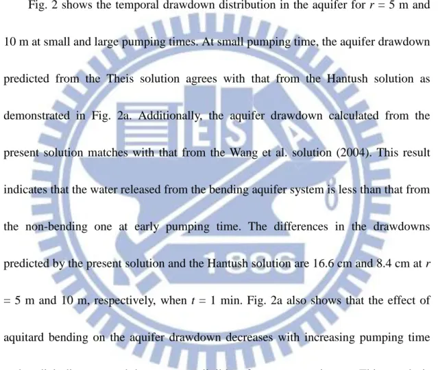
Fig. 2 shows the temporal drawdown distribution in the aquifer for r = 5 m and 10 m at small and large pumping times. At small pumping time, the aquifer drawdown predicted from the Theis solution agrees with that from the Hantush solution as demonstrated in Fig. 2a. Additionally, the aquifer drawdown calculated from the present solution matches with that from the Wang et al. solution (2004). This result indicates that the water released from the bending aquifer system is less than that from the non-bending one at early pumping time. The differences in the drawdowns predicted by the present solution and the Hantush solution are 16.6 cm and 8.4 cm at r = 5 m and 10 m, respectively, when t = 1 min. Fig. 2a also shows that the effect of aquitard bending on the aquifer drawdown decreases with increasing pumping time and radial distance and becomes negligible after twenty minutes. This result is consistent with one of the conclusions given in Wang et al. (2004). In the period from 20 to 1000 minutes, there is no obvious difference in aquifer drawdown among those four solutions. Fig. 2b shows that the present solution matches with the Hantush solution and the Theis solution agrees with the Wang et al. solution after 1000 minutes.
With considering the leakage effect, the time-drawdown curves approach a constant value for the cases with and without accounting for the bending effect. On the contrary, the aquifer drawdown keeps increasing when neglecting the leakage effect. Fig. 3 exhibits the spatial drawdown distribution for the aquifer system under pumping when subject to both the bending and leakage effects. The distance-drawdown curves indicate that bending effect is significant near the pumping well at short pumping time. On the other hand, the influence of leakage rate on the drawdown curve is more obvious at long pumping time. These results indicate that neglecting the bending effect would lead to under-estimation of drawdown at early time and ignoring the impact of leakage rate might result in over-estimation of drawdown at late time.
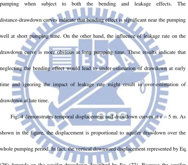
Fig. 4 demonstrates temporal displacement and drawdown curves at r = 5 m. As shown in the figure, the displacement is proportional to aquifer drawdown over the whole pumping period. In fact, the vertical downward displacement represented by Eq. (28) depends on the aquifer drawdown described by Eq. (27). Because the aquifer drawdown increases with pumping time, the vertical downward displacement also increases with pumping time.
4.2 Analysis based on dimensionless parameters
the dimensionless parameters sD, tD, and rD, which are defined assDs/(Q/4T),
) /( 4Tt s r2
tD and rDwr4/(SmD). The curves of sD versus tD at rD = 0.1 are
plotted in Fig. 5 for Sw/S ranging from zero to unity. The aquifer matrix is
incompressible when Sw/S equals unity. Under this circumstance, the present solution
reduces to the Hantush solution, which is independent of Sw/S. The aquifer drawdown
increases with aquifer skeleton compression at early pumping time. As tD is larger
than 20, the present solution agrees with the Hantush solution.
4.3 Sensitivity analysis
Sensitivity analysis provides an indication for the model output (i.e., drawdown) in response to the change of model parameter. The model parameters often have different unit and magnitude. The normalized sensitivity is commonly used to evaluate and compare the sensitivities of the model to different parameter defined as
k k i k i P P O X / , (32) where Xi,k is normalized sensitivity coefficient of the model, depending on the kth
input parameter (Pk) at the ith observation point and the derivative of the output
quantity (Oi) with respect to the Pk. The derivative term in Eq. (32) can be
approximated by the finite-difference formula as
k k i k k i k i P P O P P O P O ( ) ( ) (33) where Δ Pk is a small increment selected as 10-3 × Pk.
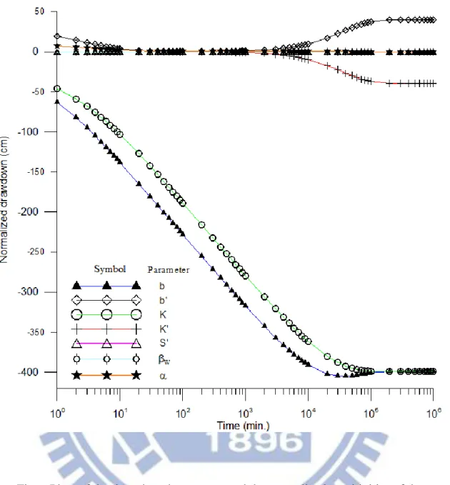
The parameters of the aquifer and aquitard used in the sensitivity analysis for the LCA subject to the bending effect are listed in Table 1. Fig. 6 shows the curves of normalized sensitivity of the aquifer drawdown to each of parameters b, b′, K, K′, α, βw
and S′. The aquifer thickness and hydraulic conductivity have obvious negative influences on the aquifer drawdown. Their effects increase with pumping time before 105 and then keep a constant magnitude after that time. For the aquitard storage coefficient and water compressibility, they have less impact on aquifer drawdown over the whole observation period. Before 20 minutes, the aquitard thickness and elastic aquifer matrix compressibility product positive influences on the aquifer drawdown, which correspond to the result in Fig. 2(a), demonstrating the impact of the bending effect. This result indicates the importance of bending effect in a LCA at early pumping time. In the period between 20 and 1000 minutes, the influences of parameters b′, K′, α,
βw and S′ on the aquifer drawdown are insignificant. After 1000 minutes, the elastic
aquifer matrix compressibility still shows minor influence and the aquitard thickness demonstrates positive impact on the aquifer drawdown. For aquitard hydraulic conductivity, its influence on aquifer drawdown is minor before 1000 minutes, and exhibits negative effect after that time.
According to the sensitive analysis, the thickness and hydraulic conductivity of the aquifer are the most influential factors on the aquifer drawdown among the
considered parameters. These two parameters present significant negative effect on the aquifer drawdown distribution. Furthermore, the thickness of the aquitard shows small positive effect at early time and large at late time and the hydraulic conductivity of the aquitard presents a large negative effect at late time. The compressibility of aquifer matrix only reveals a slightly positive effect at early time. The compressibility of water and aquitard storage display almost no influence over the whole pumping time.
CHAPTER 5 CONCLUTIONS
This thesis provides an analytical framework for understanding the drawdown distribution with the consideration of both the bending effect and leakage effect in a LCA system subject to pumping at a fully penetrating well. The mathematical model developed herein involves three equations for describing the vertical displacement in response to the bending effect and the drawdown distributions in the aquifer and aquitard. The Laplace-domain solutions of this model are derived by sequentially applying the Hankel transform and Laplace transform and the corresponding time-domain results are obtained by employing the modified Crump method. The conclusions can be drawn as follows:
1. Contrary to the traditional groundwater theory, the present solution demonstrates a larger drawdown at early pumping time due to the effect of aquitard bending and a smaller drawdown at late pumping time due to the influence of leakage rate.
2. Without the presence of aquitard leakage in a confined aquifer system, the present solution reduces to the Wang et al. solution (Wang et al., 2004), which accounts for the effect due to aquitard bending. Additionally, the Hantush solution (Hantush, 1960) has been shown as a special case of the present solution
when neglecting the effect of aquitard bending.
3. Based on the thin plate theory, the vertical downward displacement is found proportional to the aquifer drawdown. The strength of bending effect fades out as the radial distance and pumping time increases. Sensitivity analysis shows that the aquifer drawdown is sensitive to the aquifer skeleton compression only at early time; therefore, neglecting the impact of bending effect leads to overestimate of water released from the aquifer system at short pumping period.
REFERENCES
Abramowitz, M., Stegun, I.A., 1964. Handbook of mathematical functions with formulas, graphs, and mathematical tables. Dover publications, Washington, DC.
Barua, G., Bora, S.N., 2010. Hydraulics of a partially penetrating well with skin zone in a confined aquifer. Advances in Water Resources 33(12), 1575-1587. Bear, J., 1988. Dynamics of fluids in porous media. Dover Publications, Inc., New
York.
Boresi, A.P., Schmidt, R.J., Sidebottom, O.M., 1993. Advanced Mechanics of Materials. John Wiley & Sons, New York.
Boulton, N., 1954. Unsteady radial flow to a pumped well allowing for delayed yield from storage. International Association of Hydrological Sciences 2, 472-477. Boulton, N., 1963. Analysis of data from non-equilibrium pumping tests allowing for
delayed yield from storage. Ice Virtual Library, p. 469-482.
Chen, C.-X., 1974. Analytical solutions to ground water flow toward wells in a confined-unconfined aquifer (in Chinese). Beijing College of Geology, Beijing.
Chinese). Geology Publishing House, Beijing.
Crump, K.S., 1976. Numerical inversion of Laplace transforms using a Fourier series approximation. Journal of the ACM 23(1), 89-96.
de Hoog, F.R., Knight, J., Stokes, A., 1982. An improved method for numerical inversion of Laplace transforms. SIAM Journal on Scientific and Statistical Computing 3, 357.
Denis, R.E., Motz, L.H., 1988. Drawdowns in Coupled Aquifer with Confining Unit Storage and ET Reduction. Ground water 36(2), 201-207.
Hantush, M.S., 1960. Modification of the theory of leaky aquifers. Journal of Geophysical Research 65(11), 3713-3725.
Hantush, M.S., Jacob, C.E., 1955. Non-steady radial flow in an infinite leaky aquifer. Transactions, American Geophysical Union 36(1), 95-100.
Hemker, C.J., Maas, C., 1987. Unsteady-Flow to Wells in Layered and Fissured Aquifer Systems. Journal of Hydrology 90(3-4), 231-249.
Hu, L.T., Chen, C.X., 2008. Analytical methods for transient flow to a well in a confined-unconfined aquifer. Ground Water 46(4), 642-646.
Hunt, B., Scott, D., 2005. Extension of Hantush and Boulton Solutions. Journal of Hydrologic Engineering 10(3), 223-236.
Hydrologic Engineering 12(2), 146-155.
IMSL, 2003: IMSL Fortran Library User’s Guide Math/Library Vol. 2 of 2. version 5.0, Houston, Texas, Visual Numerics.
Kim, J.M., Parizek, R.R., 1997. Numerical simulation of the Noordbergum effect resulting from groundwater pumping in a layered aquifer system. Journal of Hydrology 202, 231-243.
Li, J., 2007. Transient radial movement of a confined leaky aquifer due to variable well flow rates. Journal of Hydrology 333, 542-553.
Li, Y., Neuman, S.P., 2007. Flow to a well in a five-layer system with application to the Oxnard Basin. Ground Water 45(6), 672-682.
McLachlan, N.W., 1955. Bessel functions for engineers. Clarendon Press. Moench, A.F., Prickett, T.A., 1972. Radial flow in an infinite aquifer undergoing
conversion from artesian to water table conditions. Water Resources Research 8(2), 494-499.
Sekhar, M., Kumar, M.S.M., Sridharan, K., 1994. Parameter estimation in an anisotropic leaky aquifer system. Journal of Hydrology 163, 373-391. Shanks, D., 1955. Non-linear transformations of divergent and slowly convergent
sequences. Journal of Mathematics and Physics 34, 1-42.
piezometric surface and the rate and duration of discharge of a well using ground water storage. US Dept. of the Interior, Geological Survey, Water Resources Division, Ground Water Branch.
Wang, X.S., Chen, C.X., Jiao, J.J., 2004. Modified Theis equation by considering the bending effect of the confining unit. Advances in Water Resources 27(10), 981-990.
Watson, G.N., 1958. A treatise on the theory of Bessel functions. Cambridge University Press.
Wen, Z., Huang, G.H., Zhan, H.B., 2008. Non-Darcian flow to a well in an
aquifer-aquitard system. Advances in Water Resources 31(12), 1754-1763. Yang, S.Y., Yeh, H.D., 2005. Laplace-domain solutions for radial two-zone flow
equations under the conditions of constant-head and partially penetrating well. Journal of Hydraulic Engineering ASCE131(3), 209-216.
Yang, S.Y., Yeh, H.D., 2009. Radial groundwater flow to a finite diameter well in a leaky confined aquifer with a finite-thickness skin. Hydrological Processes 23(23), 3382-3390.
Yang, S.Y., Yeh, H.D., Chiu, P.Y., 2006. A closed form solution for constant flux pumping in a well under partial penetration condition. Water Resources Research 42(5), W05502, doi:10.1029/2004WR003889.
Yeh, H.D., Lu, R.H., Yeh, G.T., 1996. Finite element modelling for land displacements due to pumping. International Journal for Numerical and Analytical Methods in Geomechanics. 20(2), 79-99.
Zhan, H., Bian, A., 2006. A method of calculating pumping induced leakage. Journal of Hydrology 328, 659– 667.
APPENDIX A: DERIVATION OF THE LAPLACE-DOMAIN SOLUTION TO
EQUATIONS (27) AND (28)
Taking the Laplace transform toEqs. (1) and (14) results in
) , ( ) , ( ) , ( ) ) , ( 1 ) , ( ( ~ ~ ~ ~ 2 ~ 2 p r p r s pS p r q r p r s r r p r s T l (A1) and ) , ( ) , ( ) , ( 1 1 ~ ~ ~ 2 2 2 2 p r s p r w S p r w r r r r r r D w m w (A2) where ( , ) ~ p r
ql is the leakage rate of the aquitard in Laplace domain and ( , )
~
p r
is an additional amount of water released from aquifer per unit time in Laplace domain. The boundary conditions of Eqs. (3), (4), (16) and (17) in Laplace domain are
0 ) , ( ~ p s (A3) Tp Q r p r s r r 2 ) , ( ~ 0
lim
(A4) 0 ) , ( ~ p w (A5) and 0 ) , 0 ( ~ r p w (A6) Substituting Eqs. (26) and (A4) into Eq. (A1) yields0 ) , ( ) , ( ) ) coth( ( ) ) , ( 1 ) , ( ( ~ ~ ' ~ 2 ~ 2 p r w p p r s p S b K r p r s r r p r s T w (A7)
Employing the Hankel transform to remove the radial distance for Eqs. (A2) and (A7) produces ) , ( ) 1 )( , ( p c 4 S s p w m (A8) and p Q p w p p s p S b K T w 2 ) , ( ) , ( ) ) coth( ( 2 ' (A9) where and the variables s(,p) and w(,p) are the aquifer drawdown and vertical downward displacement in Laplace-Hankel domain, respectively. Eq. (A8) can be rewritten as ) , ( 1 ) , ( 4 s p c S p w m (A10) Substituting Eq. (A10) into Eq. (A9), the aquifer drawdown can be expressed as
) 1 ( ) 1 ))( ' coth( ' ( 1 2 ) , ( 4 4 2 4 c S S pS c b k T c p Q p s w (A11)
The vertical downward displacement in a LCA system can be obtained after substituting Eq. (A11) into Eq. (A10) and the result in Laplace-Hankel domain is
) 1 ( ) 1 ))( ' coth( ' ( 2 ) , ( 4 4 2 c S S pS c b k T S p Q p w w m (A12)
Utilizing the inverse Hankel transform to Eqs. (A11) and (A12), the Laplace-domain solutions of the aquifer drawdown and vertical downward displacement in a LCA with considering the bending effect can be found as Eqs. (27) and (28).
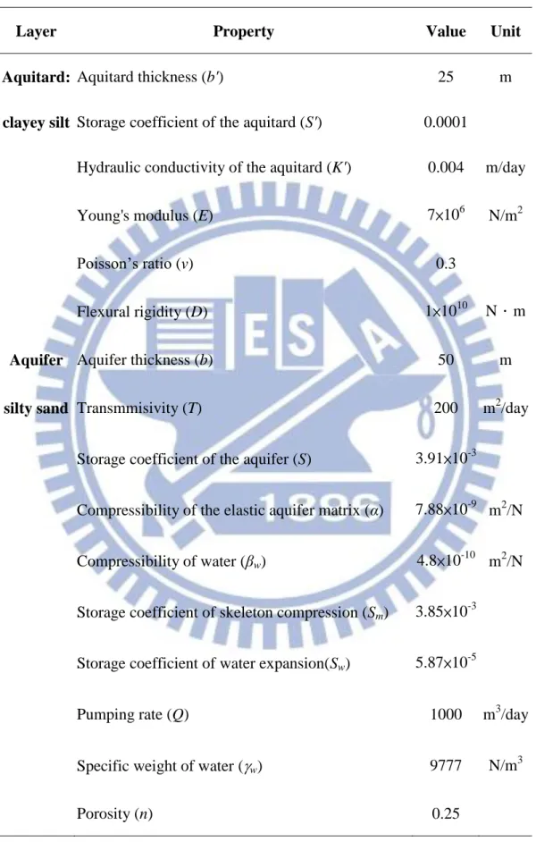
Table 1 Aquifer and aquitard properties in a leaky confined aquifer system.
Layer Property Value Unit
Aquitard: Aquitard thickness (b') 25 m
clayey silt Storage coefficient of the aquitard (S') 0.0001
Hydraulic conductivity of the aquitard (K') 0.004 m/day Young's modulus (E) 7×10⁶ N/m2
Poisson’s ratio (v) 0.3
Flexural rigidity (D) 1×10¹⁰ N.m
Aquifer Aquifer thickness (b) 50 m
silty sand Transmmisivity (T) 200 m2/day
Storage coefficient of the aquifer (S) 3.91×10⁻³ Compressibility of the elastic aquifer matrix (α) 7.88×10⁻⁹ m2/N Compressibility of water (βw) 4.8×10⁻¹⁰ m2/N
Storage coefficient of skeleton compression (Sm) 3.85×10⁻³
Storage coefficient of water expansion(Sw) 5.87×10⁻⁵
Pumping rate (Q) 1000 m3/day Specific weight of water (w) 9777 N/m3
Confined aquifer Aquitard Q z r Impermeable bed Ground surface Unconfined aquifer Drawdown, s Displacement, w z = b + b’ z = b
Piezometric head before pumping
Piezometric head during pumping Top of aquitard before pumping
Top of aquitard during pumping
Fig.1 Idealized representation of a leaky confined aquifer subject to pumping at a fully penetrating well
Fig. 2(a) Fig. 2 The time-drawdown curves for r = 5 m and 10 m (a) at small time (b) at large time.
Fig. 3 The distance-drawdown curves for the influences of bending effect and leakage effect.
Fig. 5 The curves of dimensionless drawdown sD versus dimensionless time tD at rD =
Fig. 6 Plots of the time-drawdown curve and the normalized sensitivities of the parameters K’, S’, b’, K, α, βW and b versus time.