搭配調適網格加密功能之平行化Poisson-Boltzmann方程式有限元素數值分析研究

國 立 交 通 大 學

機 械 工 程 學 系

碩 士 論 文

Parallel Implementation of Three-dimensional

Poisson-Boltzmann Equation Solver Using

Finite Element Method with

Adaptive Mesh Refinement

搭配調適網格加密功能之平行化

Poisson-Boltzmann 之方程式

之有限元素數值分析研究

研究生：鍾東霖

指導教授：吳宗信 博士

誌謝

有人說，誌謝是整各碩士論文中最難寫的一章，我想其中的困難點可能就是 因為要在有限的篇幅中，表達出心中內心的感動與感謝。此時，我有深刻的體驗。 兩年的光陰，速度快到我渾然不覺，還在驚訝中，人生就到了新的開端。在風城 的兩年中，遭遇的事情，每件都是直得一再回味與思考。有喜有悲，有錯有對， 每種心情都是我成長的元素。 在碩士兩年中，感謝吳宗信老師在這兩年中的教誨，不管是學術上的指導還 是在處事上的叮嚀，都讓我學習到很多，感謝老師在這兩年中的照顧。同時也感 謝口試委員傅武雄教授、郭添全博士在口試時提供的寶貴意見。 感謝邵董，在我混亂的時候，給我面對困難的方向；感謝曾董在我害怕的時 候給我的勇氣；感謝國賢老大與在學習上的大力幫忙，這份論文沒有你的幫忙根 本不會存在；感謝連又永學長在後期學習上的大力支援。接著感謝 CFD 車隊的大 箭頭，李允民；對你的感謝實在是不知道怎麼寫，我想等我有一天贏過你後，我 在大聲的跟你說我的感謝好了。感謝柏誠，立軒，姝吟，在這兩年中的互相扶持， 一起熬夜，互相打屁與分享喜悅，共同參與的這份回憶我會謹記在心。也謝謝 MUST 所有成員，謝謝你們的幫忙。 此外也感謝我的好朋友們，正偉、仲雍、大塊、永霖、卡川、俊傑、阿國、 阿呆、肉祥、老江、繩子、小偉等。謝謝你們給我的一切。 最後，獻上最由衷的感謝給我的家人與女友，由於你們的鼓勵與支持，才能 使我有無後顧之憂的求學。 鍾東霖 謹誌 乙酉年七月於風城交大

搭配調適網格加密功能之平行化 Poisson-Boltzmann 之方程式

之有限元素數值分析研究

學生:鍾東霖 指導教授 : 吳宗信

國立交通大學機械工程學系

摘要

本研究完成平行化三維 Poisson-Boltzmann 之程式建立，主要是利用有限元 素法搭配 Monotone iteration 處理非線性項的部份，搭配本實驗室發展的平行化 調適網格模組，將需要加密的區域，做適當的加密。在程式的驗證上，主要是以 模擬圓球體，圓柱體的電雙層電位分佈，在和解析解與文獻中發表的近似解做比 較。,於邊界電位等於一的情形下，解析解，模擬解與近似解，三者的結果一致， 由此可驗證程式的正確性。驗證完程式的正確性後，再將本程式與平行化調適網 格做搭配後模擬兩顆帶電離子於無限遠空間內的電雙層電位分佈，將結果與歷年 的文獻做比較，經歷五個階段的網格加密後，計算電位，電場值與作用力後，比 較文獻上的資料，大約有 0.06%的誤差。於後，模擬兩帶電離子於圓柱型電洞內 的電雙層電位分佈，計算並比較作用力值後，與文獻上的資料大約有 1%上的誤 差，這些誤差推測是網格的緊密度不足所導致，但因電腦資源的問題，網格也無

法再繼續加密下去。在文獻中，都是以二階以上的有限元素分析電雙層電位，在 未來如能提高本程式的有限元素階數，相信可以獲得更有效率，更精準的分析。

此程式可用來解析電雙層內的電位分布，也可解析膠體間的交互作用力的分 析。對於電滲流分析及薄膜效率分析上，都有不錯的應用。

Parallel Implementation of Three-dimensional Poisson-Boltzmann

Equation Solver Using Finite Element Method

with Adaptive Mesh Refinement

Student :

Tung-Lin Jung Advisor : Dr. Jong-Shinn Wu

Institute of Mechanical Engineering National Chiao Tung University

Abstract

A parallel Poisson Boltzmann equation solver using finite element method with adaptive mesh refinement is proposed. A Monotone iterative method was used to solve the nonlinear equation arising from the finite element discretization procedure. A 3D Poisson-Boltzmann equation was used to model the electric double layer field. And the solver will be using to simulate this phenomenon. First, in order to verify code accuracy we model the EDL potential distribution at sphere and cylinder, and compared with analytical solution and approximant solution. These results are all the same in small zeta potential. After verification, we couple with parallel adaptive mesh refinement to compute some simple cases such as two identical charged spherical particles and computer the interaction force. After five step refinement levels, we calculate the potential, electric field and interaction force, and compared with previously literature. It has 0.06% inaccuracy between our results and previously

work. After this case, we apply our code to simulate the situation of two identical particles in a cylindrical pore, and compared with previously works. It also has 1% inaccuracy. The mesh distribution may influence the result, but we can not refine mesh after five level according to computing resources. In the previously works, most of them are use high order finite element method. If we can use high level mesh in future, we can have more accuracy result.

INDEX

摘要...I Abstract...III INDEX...V LIST OT TABLE AND FIGURES ...VI

Chapter 1 Introduction... 1

1-1 Motivation ... 1

1-2 Background ... 2

1-2.1 The Like-charge Attractions Phenomenon ... 2

1-2.2 Electric double layer ... 2

1-3 Literature Survey... 4

1.4 Objectives and Organization of the Thesis... 5

Chapter 2 The Numerical Method ... 6

2-1 The Poisson-Boltzmann Equation for the EDL Potential Ψ ... 6

2-2 Discretization Using Finite Element Method ... 7

2-3 Force Calculations ... 12

2-4 Conjugate Gradient Method for Linear Algebra Equation... 13

2-5 Monotone Iterative Methods ... 16

2-6 Parallel Implementation of the P-B Equation Solver... 17

2-6.1 Introduction to Parallel Distributed Computing ... 17

2-6.2 Parallel Implementation... 18

2-7 Parallel Adaptive Mesh Refinement ... 19

2-7.1 The Basic Algorithm of Parallel Adaptive Mesh Refinement... 19

2-7.2 Cell Quality Controls... 20

2-7.3 Procedures of Parallel Mesh Refinement ... 22

2-8 Coupling Procedures of Parallel P-B Equation Solver with PAMR ... 25

2-8.1 Refinement Parameter and Criteria ... 25

2-8.2 Parallel Poisson-Boltzmann Solver with Mesh Refinement... 26

Chapter 3 Results and Discussion... 27

3-1 Code Verifications... 27

3.1-1 Potential Around a Sphere ... 27

3.1-2 Potential Around a Cylinder ... 28

3-2 Simulation of Two Interacting Identical Particles Coupled with PAMR .... 29

3-3 Two Identical Particles in a Cylindrical Pore ... 30

Chapter 4 Future Work ... 31

4-1 Summary ... 31

4-2 Recommendations for Future Work ... 31

References ... 32

Table ... 35

LIST OT TABLE AND FIGURES

Table3-1: Steps of the adaptive process:... 35

Table3-2: Steps of the adaptive process for previously literature [6] ... 36

Table3-3: The interaction forces of two particles in a cylinder pore at different separation distance. ... 36

Fig 1.1 The illustration of like-charge attractions phenomenon ... 38

Fig 1.2 The Electric Double Layer distribution ... 39

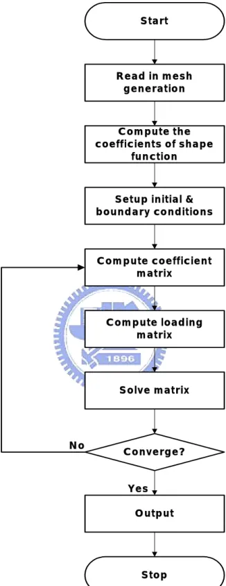
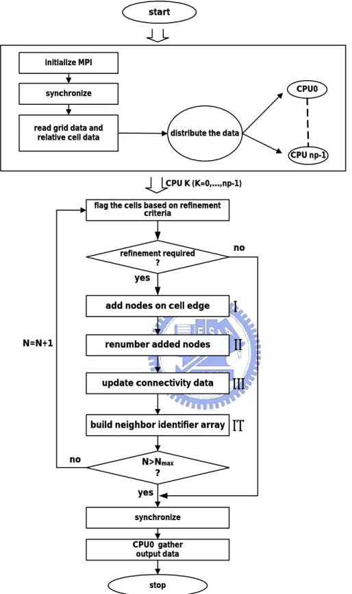
Fig 2.1 Simplified flow chart of the three-dimensional nonlinear Poisson-Boltzmann solver ... 40

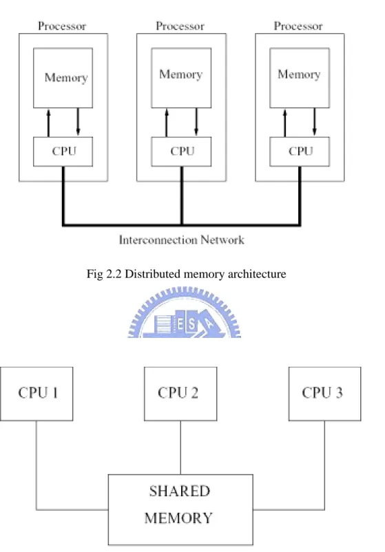
Fig 2.2 Distributed memory architecture ... 41

Fig 2.3 Shared memory architecture ... 41

Fig 2.4 Flow chart of parallel Poisson-Boltzmann solver... 42

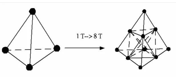
Fig 2.5 Isotropic mesh refinement of tetrahedral mesh (T: Tetrahedron) ... 43

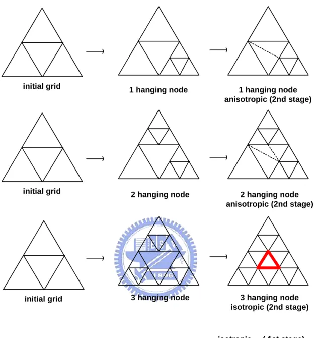
Fig 2.6 Mesh refinement rules for two-dimensional triangular cell ... 44

Fig 2.7 Schematic diagram for mesh refinement rules of tetrahedron... 45

Fig 2.8 Schematic diagram of the proposed cell quality control ... 46

Fig 2.9 Schematic diagram of typical cell quality control ... 47

Fig 2.10 Schematic diagram of simple cell quality control ... 48

Fig 2.11 A case that the proposed cell-quality-control would not affect to it ... 49

Fig 2.12 Flow chart of parallel mesh refinement module ... 50

Fig 2-13 Flow chart of moduleⅠ ... 51

Fig 2-14 Coupled PPBS-PAMR method... 52

Fig 3.1 Geometry of the potential around a sphere case... 53

Fig 3.2 The comparison of different result at Ψ =1(sphere)... 54

Fig 3.4 The relationship between iteration and residual with different initial

guess (Ψ =5) ... 56

Fig 3.5 Geometry of the potential around a cylinder case ... 57

Fig 3.6 The comparison of different result at Ψ =1(cylinder)... 58

Fig 3.7 The comparison of different result at Ψ=5(cylinder) ... 59

Fig 3.8 The illustration the case of two interacting identical particles ... 60

Fig 3.9 Level 0 initial mesh of two interacting identical particles case... 61

Fig 3.10 Level 1 refinement mesh of two interacting identical particles case.. 62

Fig 3.11 Level 2 refinement mesh of two interacting identical particles case.. 63

Fig 3.12 Level 3 refinement mesh of two interacting identical particles case.. 64

Fig 3.13 Level 4 refinement mesh of two interacting identical particles case.. 65

Fig 3.14 Level 5 refinement mesh of two interacting identical particles case.. 66

Fig 3.15 The potential distribution of two identical particles ... 67

Fig 3.16 The potential distribution for the sphere confined in a pore at separation distances h=0.5 ... 68

Fig 3.17 The potential distribution for the sphere confined in a pore at separation distances h=6 ... 69

Fig 3.18 Potential along the midplane between two spheres ... 70

Chapter 1

Introduction

1-1 Motivation

The study of fluid flow in microchannels is of significant interest to engineers because of microfluid have wide industrial applications. For examples, miniaturize flow injection analysis, micro-reactors for the analysis of biological cells, heat sinks for the analysis of biological cells, and heat sinks for cooling microchips and laser diode arrays, etc.

At the small scales channels, the electrical double layer (EDL) phenomena significantly makes an influence on the fluid behaviors and the electrical double layer is also the important interfacial effect.

The EDL field in such a microchannels is governed by the Nonlinear Poisson-Boltzmann (PB) equation.

The Nonlinear Poisson-Boltzmann equation is also used for the description of the distribution of electrostatic potential in colloidal dispersions. Knowing the electrostatic potential, one can calculate other quantities such as the force of particle-particle interaction. Features of particle interaction are great importance for the stability and properties of colloidal dispersions. Numerical investigation of models based on the PB equation can provide important information on effective particle interaction in colloidal systems.

In previous documents and theses, there are not so many reports discussed the three-dimensional computation model. The two-dimensional computation model was most commonly mentioned. However, when the geometries is getting complex, the two-dimensional computation model is gradually losing its accuracy.

Therefore, we have developed a numerical scheme to simulate Electrical double layer potential distribution by solving 3D Nonlinear Poisson-Boltzmann equation.

1-2 Background

1-2.1 The Like-charge Attractions Phenomenon

Colloidal sphere provide a simple model system for understanding the interactions of the charge particles in a salt solution. Hence, it came as a great surprise when it was observed that two like-charge spheres can attract each other when the spheres are confined by walls. Since both the charge densities and sizes of the spheres are in the range of large proteins, it would be expected that a charge in sign of this interaction would have important implications for biological systems.

The attractive interaction between two charge walls can be understood with a simple picture (Fig 1.1). When the spheres are sufficiently close to the wall, they are electrostatically repelled from it. The net force on each sphere thus includes both their mutual electrostatic repulsion and their repulsion from the wall. How the spheres respond depends on their hydrodynamic mobility: when the spheres are close together, their mutual repulsion overwhelms any hydrodynamic coupling, and the spheres will separate as hydrodynamic coupling; the spheres will separate as expected for like-charge bodies. However, when they are beyond some critical separation, the hydrodynamic coupling due to the wall force overcomes the electrostatic repulsion, so that the relative distance between the spheres decreases as they move away from the wall.

1-2.2 Electric double layer

Electrokinetic phenomena are of considerable importance in many fields of science and engineering. In particular, they exert a strong influence on the flow behavior of a fluid in microchannels and capillaries. Most solid surfaces bear electrostatic charges. When a charge surface is in contact with an electrolyte, the

electrostatic charges on the solid surface will influence the distribution of nearby ions in the electrolyte solution. Ions of opposite of charges to that of the surface are attracted towards the surface, while ions of like charges are repelled from the surface; thus, an electric field is established. The charges on the solid surface and the balancing charge in the liquid are called the “electric double layer” (EDL). The EDL potential distribution is show in Fig 1.2. The sign and magnitude of the EDL field depend on the nature of the surface and the liquid.

The distribution of EDL can be class with two regions. One is compact or stern

layer the other is diffusion layer. Guoy and Chapmal modeled the region near the

surface as a diffuse double layer, where they linked the nonuniform ion distribution to

the competing electrical and thermal diffusion forces [1]. Stern later presented the

basis for the current model, in which the Stern plane splits the EDL into an inner, compact layer and an outer, diffuse layer. In the inner layer or the Stern layer, the geometry of the ions and molecules strongly influences the charge and potential distribution, with the Stern plane located near the surface, at roughly the radius of a hydrated ion. The inner layer between the surface and the Stern plane is considered to be immobile; if the ions are within the Stern plane, thermal diffusion will not be strong enough to overcome electrostatic or Van der Waals forces and they will attach

to the surface, becoming specifically adsorbed [1]. In the outer diffuse layer, the ions

are far enough away from the surface that they are mobile. Electrokinetic transport phenomena such as electroosmosis can be understood in terms of the surface potential at the surface of shear, because these phenomena are only directly related to the

mobile part of the EDL [1].

Within the diffuse layer, because of the EDL, the net charge density ρ_e is not

exerted on the ions in the diffuse layer of the EDL. The ions will move under the influence of the applied electrical field, pulling the liquid with them and resulting in electroosmotic flow. The fluid movement is carried through to the rest of the fluid in the channel by viscous forces. This electrokinetic process is called electroomosis.

1-3 Literature Survey

The EDL field is described by the Poisson-Boltzmann equation, which is a three-dimensional, nonlinear, second-order partial differential equation. The hyperbolic sine term makes the second-order different equation exponentially nonlinear; therefore. A general analytical solution is not possible.

The PB equation can model many phenomenon such as the like-charge interaction, electrokinetic flow and micro-fluidic actuation etc. There are many studies in the literature dealing with the solution of Poisson-Boltzmann equation.

Bowen and Sharif [2] they presented a 2D FE solution combined with adaptive

mesh refinement. They used the Debye-Huckel solution to initial guess, and the Newton sequence was used to solve the nonlinear hyperbolic sine term. They used nine-node quadrilateral elements. Bowen and Sharif also presented some results in

1998 journal of Nature [3]. They said their solver can model the like-charge

attractions phenomenon which is presented in 1997 journal of Nature by Larsen and

Grier [4]. Dyshlovenko [5] also presented a 2D FE solution combined with adaptive

mesh refinement but they used six-node triangular elements. In 2002, Dyshlovenko

publish their result in CPC [6], but Dyshlovenko is different from Bowen and Sharif,

Dyshlovenko do not find the like-charge attractions phenomenon in his results.

Tuinier [7] proposed the approximate solutions to the PB equation in spherical and

solver. Das and Bhattacharjee [8] examine the results in 2004, they presented finite

element simulation results which is considered the roughness on the wall. They think roughness on the wall can influence the electrostatic forces and the like-charge attraction.

1.4 Objectives and Organization of the Thesis

Based on previous reviews, the current objectives of the thesis are summarized as follows:

1. To develop a parallel 3-D finite-element solution of the nonlinear

Poisson-Boltzmann equation.

2. To couple the parallel adaptive mesh refinement with this PB solver.

The organization of this thesis would be stated as follow: First is this introduction, followed by the numerical method. Next would be the Results and discussions, and finally the Conclusions and Future work.

Chapter 2

The Numerical Method

This study uses a computer simulation code, which is developed by Kuo-Hsien Hsu, MUST, NCTU. The simulation code is three-dimensional, finite-element, nonlinear Poisson Boltzmann. General flowchart of the simulation is shown in Fig.

2.1.

2-1 The Poisson-Boltzmann Equation for the EDL Potential Ψ

Consider a liquid phase containing positive and negative ions in contact with a planar negatively charged surface. An EDL field will be established. According to the theory of electrostatics, the relationship between the electrical potentialΨ and the net

charge density per unit volume ρ_e at any point in the solution is described by the

three-dimensional Poisson equation.

0 2 2 2 2 2 2 εε ρ ψ ψ ψ _e z y x ∂ =− ∂ + ∂ ∂ + ∂ ∂ [2-1] e

ρ is the charge density, ε is the dimensionless dielectric constant of the solution,

and ε_o is permittivity of vacuum. For any fluid consisting of two kinds of two kinds

of ions equal and opposite charge (z+ and z-), the number of ions of each type is given

by the Boltzmann equation.

) / exp( ), / exp( ₀ 0 ze k bT n n ze k bT n n− = ψ _b + = − ψ _b [2-2]

n+ and n- are the concentrations of the positive and negative ions, n0 is average

concentration of ions, exp(zeψ /k_bbT) is the Boltzmann factor, kb, and T is the

absolute temperature. The Boltzmann distribution is applicable only when the system is in the thermodynamic equilibrium state.

Then the net charge density in a unit volume of the fluid is given by: ) / sinh( 2 ) (n n ze n0ze zeψ kbT ρ = + − − =− [2-3] Substituting Eq. [2-3] in Eq. [2-1], we can get a nonlinear second-order three-dimensional Poisson-Boltzmann equation:

      = ∂ ∂ + ∂ ∂ + ∂ ∂ T k ze ze n z y x _b o ψ εε ψ ψ ψ sinh 2 0 2 2 2 2 2 2 [2-4]

Nondimensionalizing the above equation via

T k ze z z y y x x b ψ ψ κ κ κ = = = = ₂ , ₂ , ₂ , [2-5] We obtain a dimensionless form of Eq. [2-4] that can be written as

( )

ψ ψ ψ ψ sinh 2 2 2 2 2 2 = ∂ ∂ + ∂ ∂ + ∂ ∂ z y x [2-6]

Where,κ2 =2n₀z2e2/εε₀k_bT is the Debye-Huckel parameter, and 1/κ is the 2

characteristic of the EDL.

2-2 Discretization Using Finite Element Method

The FEM is the computer-aid mathematical technique for obtaining approximate numerical solution to the abstract of calculus that predicts the response of physical system subjected to the external influences.

Such problems arise in many areas of engineering, science, and applied mathematics. Applications to date have occurred principally in the areas of solid mechanics, heat transfer, fluid mechanics, and electromagnetism.

1. The domain is divided into smaller regions called elements. Adjacent elements touch without overlapping, and there are no gaps between the elements. The shapes of the elements are intentionally made as simple as possible.

2. In each element the governing equations, usually in differential or variation

(integral) form, are transformed into algebraic equation. The element equations are algebraically identical for all elements of the same type, which usually need to be derived for only one or two typical elements.

3. The resulting numbers are assembled (combined) into a much larger set of

algebraic equations called the system equations. Such huge systems of equations can be solved economically because the matrix of coefficients is “spares”.

4. Solved the matrix problem.

FEM seeks an approximate solutionU~, an explicit expression for U, in terms of

known functions, which approximately satisfies the governing equations and boundary conditions. It obtains an approximate solution by using the classical trial-solution procedure. Normally, it is not possible to obtain strong solutions for the problem at hand. Instead one usually decretive the otherwise continuous problem and obtain so-called weak solutions; weak in the sense of approximate.

Now we star to derive the 3D Nonlinear Poisson solver formulation via FEM method. Consider Eq. [2-6]

( )

ψ ψ ψ ψ sinh 2 2 2 2 2 2 = ∂ ∂ + ∂ ∂ + ∂ ∂ z y x

Step1: We use ψ~ to approximateψ , then we set the trial solution:

∑

= = 4 1 ) ( ) ( * ) , , ( ~ j j e e _{N x y z a} j ψ [2-7]

(

x y z

)

N_j , , are known functions called trial functions (basis).

The purpose is to determine specific numerical values for each of the parameters

a. We use the Galerkin method. For each parameter aj we require that a weighted average of R (x, y, z; a) over the entire domain be zero. The weighting functions are trial functions N

(

x,y,z

)

associated with each aj.

Step2: Galerkin residual method

( )

Ω = Ω       ∂ ∂ + ∂ ∂ + ∂ ∂

∫

∫

ΩN _{x y z} d ΩN d e i e i ψ ψ ψ ψ sinh * * ₂ ( ) 2 2 2 2 2 ) ( [2-8]

The Galerkin residual method is a weighting residual method, which uses the trial

function as the weighting function.N is not only the weighting function, but also the _i

shape function.

Where the integral

∫

Ω

Ω d means integrate over the volume of element. We use

tetrahedral element, which have four degree of freedom (DOF). The tetrahedral element’s shape function can desired as:

(

)

1~4 6 1 * * * * ) ( _{= + + + =} i z d y c x b a V N_ie _{i i i i} And m m m l l l k k k j j j m m l l k k m m l l k k m m l l k k m m m l l l k k k z y x z y x z y x z y x V y x y x y x d z x z x z x c z y z y z y b z y x z y x z y x a_{i i i i} 1 1 1 1 1 1 1 1 1 1 1 1 1 * * * * = − = = − = = [2-9]

Step3: Integrated by part

∫∫∫

∫∫∫

∫∫∫

∑

∑

=         ∂ ∂ ∂ ∂ +         ∂ ∂ ∂ ∂ +         ∂ ∂ ∂ ∂ −       ∂ ∂ ∂ ∂ +       ∂ ∂ ∂ ∂ +       ∂ ∂ ∂ ∂ dxdydz N dxdydz z N z y N y x N x dxdydz N z z N y y N x x e e e e e e e e e e e e e e j i i i i i i i i ) ~ sinh( * ~ ~ ~ ~ ~ ~ ) ( ) ( ) ( ) ( ) ( ) ( ) ( ) ( ) ( ) ( ) ( ) ( ) ( ) ( ψ ψ ψ ψ ψ ψ ψ [2-10]

Step4: Gauss divergence theorem

Use Gauss divergence theorem to Eq. [2-10].

∫∫∫

∫∫∫

∫∫

∑

∑

=         ∂ ∂ ∂ ∂ +         ∂ ∂ ∂ ∂ +         ∂ ∂ ∂ ∂ − ⋅       ∂ ∂ + ∂ ∂ + ∂ ∂ dxdydz N dxdydz z N z y N y x N x dxdy n N k z j y i x e e e e e e e e i e e e j i i i i i ) ~ sinh( * ~ ~ ~ ˆ * ˆ ~ ˆ ~ ˆ ~ ) ( ) ( ) ( ) ( ) ( ) ( ) ( ) ( ) ( ) ( ) ( ψ ψ ψ ψ ψ ψ ψ [2-11]

Take trial function [2-7] into Eq. [2-11] then we can get Eq. [2-12]

∫∫∫

∫∫∫

∫∫

∑

∑

=         ∂ ∂ ∂ ∂ +         ∂ ∂ ∂ ∂ +         ∂ ∂ ∂ ∂ − ⋅         ∂ ∂ + ∂ ∂ + ∂ ∂ dxdydz N dxdydz z N z a N y N y a N x N x a N dxdy n N k z a N j y a N i x a N e e e j e e j e e j e e j e j e j e j i i i j i j i j i j j j ) ~ sinh( * * * * ˆ * ˆ * ˆ * ˆ * ) ( ) ( ) ( ) ( ) ( ) ( ) ( ) ( ) ( ) ( ) ( ) ( ψ [2-12] We let         ∂ ∂ + ∂ ∂ + ∂ ∂ − = k z a N j y a N i x a N e _j j e j e j j j * _ˆ * _ˆ * ˆ ˆ ) ( ) ( ) ( τ [2-13]

And Eq. [2-12] can be rewrote as follows,

dxdy N dxdydz N dxdydz a z N z N y N y N x N x N n e i e e j e e e e e e j i i i j i j i j

∫∫

∫∫∫

∫∫∫

∑

∑

− − =                 ∂ ∂ ∂ ∂ +         ∂ ∂ ∂ ∂ +         ∂ ∂ ∂ ∂ τ ψ( ) ( ) ) ( ) ( ) ( ) ( ) ( ) ( ) ( ) ~ sinh( * [2-14]

(

)

dxdy N dxdydz N dxdydz a d d c c b b V n e i e e i j j i j i j i i j

∫∫

∫∫∫

∫∫∫

∑∑

− − = + + = = τ ψ( ) ( ) ) ( * * * * * * 2 4 1 4 1 ) ~ sinh( * * 36 1 [2-15] And V dxdydz=

∫∫∫

[2-16] Take [2-16] into [2-15] Then

(

)

dxdy N dxdydz N a d d c c b b V n e i e e i j j i j i j i i j

∫∫

∫∫∫

∑∑

− − = + + = = τ ψ( ) ( ) ) ( * * * * * * 4 1 4 1 ) ~ sinh( * * 36 1 [2-17] We let

(

* * * * * *

)

) ( * 36 1 j i j i j i e _{b b c c d d} V K ij = + + [2-18] dxdy N dxdydz N F e _n i e i e e i =− ψ

∫∫∫

−

∫∫

τ ) ( ) ( ) ( ) ( ) ~ sinh( [2-19]

Finally we can get the matrix form of the Poisson-Boltzmann Equation.

{ } { }

a F e n K e j e j e ij ] :1~ [ () () = ( ) [2-20] The matrix problem of the Galerkin method is not simple to take numerically. To obtain an accurate solution it is often necessary to employ a fine mesh containing

many elements. The N×N matrix of Eq. [2-20] thus becomes very large. This

sparsity is utilized fully when implementing good computer codes for the finite element method. The sparsity leads to a significant reduction in memory requirements since only the non-zero matrix elements need to be stored together with an index of where they are stored. Moreover, the sparsity implies a huge reduction in the number of arithmetic operations needed to solve the problem. For a full matrix problem this

direct-banded matrix schemes, or iterative methods like conjugate gradient methods

or multi-grid methods, it can be reduced to becoming proportional to N2 or even

N .

2-3 Force Calculations

From the potential distribution obtained by solving the Poisson-Boltzmann equation, the electrostatic force on the spherical particles is calculated by integrating the total stress tensor, defined as

] 2

1 [EE E EI

T_ij =∆∏+ε − ⋅ [2-21]

Where E =−∇ψ is the electric field vector; I represents the identity tensor, and

∏

∆ is the osmotic pressure difference between the electrolyte at the particle surface

and bulk solution, ∆ can defined as ∏

∆∏=2n_bkT

(

coshψ −1

)

[2-22]

Where n is the bulk ion number density of the electricity neutral electrolyte. _b

We took integral the stress tensor over the surface of a particle, defined as

=

∫

⋅

S

ij ndS

T

F [2-23]

Here Fis the force acting on the spherical particle. We note here that the stress

tensor is calculated from the potential but the force on the sphere also includes a contribution from the osmotic pressure generated by the electric field; however, pressure variation due to the field at the sphere surface is normally canceled by

electrical effects so that we can assume the ∆ term is zero. Where n is the unit ∏

outward surface normal, and the subscript Srepresents integration over the closed

or on the midplane for the case of two identical spherical particles.

2-4 Conjugate Gradient Method for Linear Algebra Equation

In the linear system Ax = b suppose the coefficient matrix A is symmetric and positive definite. Solving Ax = b is equivalent to minimizing the quadratic

functionQ

( )

x = xTAx−xTb

2 1

. The conjugate gradient method is based on the idea

that the convergence to the solution could be accelerates if we minimize Q over just

the line that points down gradient. To determine xi+1 we minimize Q over

) ,... , , ( 0 1 2 i o _{span p p p p} x +

where the p represent previous search directions. An added advantage to this k

approach is that, if we can select thep to be linearly independent, then the dimension k

of the hyperplane will grow one dimension with each iteration of the conjugate gradient method. This would imply that (assuming infinite precision arithmetic) the

solution of the linear system Ax=b would be obtained in no more than N steps,

where N is the number of unknowns in the system.

Let x0 be an initial estimate to the solution ofAx=b. For our first search

direction we proceed down a Q-gradient and choose

0 0 0 1 p α x x = + [2-24] Where

( )

x b Ax Q r p0 = 0 =−∇ 0 = − [2-25] From the discussion of the method of steepest descent, we have

0 0 0 0 0 0 0 0 0 Ap p p r Ar r r r α ⋅ ⋅ = ⋅ ⋅ = [2-26] To understand what follows in the description of the conjugate gradient method, it is

important to note that 0 0 1 0 1⋅_r =_r ⋅_p = r

Rather than try to establish the above orthogonality relation with a calculation,

use the following calculus argument. By definition, r is the gradient of Q at1 x1,

where x1 is the conjugate gradient estimate to follow the initial guessx0. Also,

0

0 _p

r = is the search direction along the linex0 +α₀p0. Calculus tells us that the

gradient of Q at x1must be orthogonal to the search direction.

Not as a proof of the last statement about calculus and orthogonality, but to motivate the statement, consider the layers of an onion to be surfaces of Q = constant. Imagine piercing the onion with a skewer. In general, the skewer will pass through several outer layers of the onion, tangentially touch one of the inner layers, and again pass through the other layers and then exit. The innermost layer that the skewer touches tangentially is given by

( )

_x1 _x1

Q =

∇ [2-27] and the direction of the skewer is r0 = p0.

The conjugate gradient method calls for defining successive approximates by

i i i i _{x α p} x+1 = + [2-28] i i r i _{r β p} p+1 = +1+ [2-29]

with the scheme for choosing α and _i β to be discussed next. The things to keep in _i

mind when choosingα and _i β are: _i

1. We want the span of the search directions to fill the space we are searching as the number of iterations increases.

2. Searching down Q-gradients was basically a good idea. But, to guarantee linearly independent successive search directions, we generally need to choose conjugate

gradient search directions to be perturbations of steepest descent search directions.

We have already how to define p and0 α , so 0

1

x and r and 1 r1 =b−Ax1 can be considered known. To take the next step using the conjugate gradient method, we

must determine values for α and ₀ β so that we can calculate ₁ p and1 x2. Then we

will see a pattern emerge.

In taking this next step in the conjugate gradient method we are seeking to minimize Q over the plane,

(

1

)

0 , p p span x ₊ o [2-30]

this means that the residual r will have to be orthogonal to both 2 p and0 p . The 1

orthogonality condition p0⋅ r2 =0 will help us set the search directionp . 1

( )

0 1 1 1 0 1 0 2 0 ] [b Ax p r α p Ap p r p ⋅ = ⋅ − = ⋅ − ⋅ [2-31]

which is zero provided 0 1 0 1p ⋅ Ap = α [2-32] Definition:

Two vectors u and v are said to be A-conjugate if u⋅ Au=0.

From the requirement thatp0⋅ r2 =0, it follows that the search direction p . 1

Must be A- conjugate to the search directionp . We can now set 0 β as follows: 0

0 0 1 1 _{r β p} p = + Implies 0 0 1 1 Ap β Ar Ap = + Now 0 0 0 1 0 1 0 0= p ⋅Ap = p ⋅Ar +β p ⋅Ap Implies

0 0 1 1 0 0 1 0 0 Ap p Ar r Ap p Ar p β ⋅ ⋅ − = ⋅ ⋅ − =

Having decided to proceed from x1to x2 along the search direction defined

byp1 =r1+β₀p0, the same calculus argument used to determine gives

1 1 1 1 1 Ap p p r α ⋅ ⋅ =

So a step of the conjugate gradient method is complete.

2-5 Monotone Iterative Methods

The method of monotone iterations is a classical tool for the study of the existence of the solution of nonlinear PDE of certain types. It is also useful for the numerical solution of nonlinear types of problems approximated, for instance, by the finite difference, finite element or boundary element method. It is a constructive method that depends essentially on only one parameter, called the monotone parameter herein, which determines the convergence behavior of the iterative process. Based on adaptive 1-irregular finite element meshes, we extend this classical method

to device simulation the Poisson Boltzmann equation [9]. Compared with the NI

method, the MI method requires no Jacobian matrix and does not encounter any convergence problems and numerical difficulties. Furthermore, the MI algorithm is practical, easy in implementation, and inherently parallel for large-scale 3D simulation.

Consider an example−∇u=eu, after discretization using Finite Element Method.

We can get Eq. [2-33]

)} ( { } ]{ [A U = F U [2-33]

) ( ' _U F i i =− λ [2-34] then set the monotone iterative form, which show as

} }{ ]{ [ )} ( { } }{ ]{ [ } ]{ [A Un 1 I n Un 1 F Un I n Un i i λ λ = + + + + [2-35] where variable with subscript n represents one value obtained on previous iteration.

2-6 Parallel Implementation of the P-B Equation Solver

2-6.1 Introduction to Parallel Distributed Computing

A parallel computer, as defined by Almasi and Gottlieb [10], is a collection of

processing element that cooperate and communicate to solve large problems fast. Parallel computers can be viewed as a collection of processors and memory units which are connected by an interconnection network. The purpose of parallel computing is to get work done in less time and also to solve problems which can not fit in a single computers memory.

There are two main architectural paradigms associated with parallel computing:

Distributed memory and Shared memory [11]. In Distributed Memory architecture

parallel computers, memory is physically distributed among processors; each local memory is directly accessible only by its processor. Synchronization is achieved by moving data between processors by a fast interconnection network, see Fig2.2

In Shared memory architecture parallel computer the same memory is accessible by multiple processors. All processors associated with the program access the same

storage as shown in Fig2.3.

In our laboratory, we had setup PC Clusters which are use distributed memory system. The advantage of this kind of architecture is that it is scalable to a large number of commodity processors. A major concern with this scheme is data decomposition; the data being operated should be divided equally to balance the load,

and also should be done in a efficient manner in order to minimize communication. The scalability depends on the type of interconnection between the processors.

2-6.2 Parallel Implementation

In order to parallelize the Poisson-Boltzmann solver, we use Message Passing Interface (MPI) to be the basic toll. MPI is a library specification for message-passing, proposed as a standard by broadly based committee of vendors, implementers, and users. MPI library of a set of standard subroutine calls which allow parallel programs to be written in distributed memory system. We use Metis to distribute the cells and nodes. Running the solver to test and verity on PC Cluster belongs to our MuST laboratory. In distributed parallel finite element analysis, the domain considered is first decomposed into a number of subdomains. Then in general, one processor is assigned for each subdomain, though other variations are also possible. Computations are then performed on each processor on the local subdomain and communication takes place with the other processors whenever needed. The domain might be divided into a set of overlapping subdomains in which case Overlapping Schwartz methods are used for the solution of system. If the domain is partition into a set of non-overlapping subdomains then the methods used are called iterative substructuring methods. The two basic types of non-overlapping domain decomposition methods used in the finite element methods are the subdomain-by-subdomain and Schur

complement method [11]. The first approach is based on multi-element group

partitioning of the entire domain. The global stiffness matrix is stored as a partitioned matrix and the dominant matrix-vector operations of the stiffness matrix and the precondition solutions in the iterative algorithm are performed on the subdomain-by-subdomain basis. In the second approach the iterative algorithm is applied to the interface problem after first eliminating the internal degrees of freedom.

In our parallel system, we use the non-overlapping subdomains.

Fig 2.4 illustrates the flow chart of parallel Poisson-Boltzmann solver (PPB).

Detail is described step by step in the followings.

1. Setup initial grids and input data for every processor.

2. Initialize MPI and synchronize all processors to prepare for parallel computation.

3. Compute the coefficients of shape functions. 4. Setup initial and boundary conditions

5. Compute each processor’s coefficient matrix and communications among processor.

6. Compute each processor’s loading matrix and communications among processor.

7. Solve each processor’s matrix and communications among processors

8. To determine results of potential converge or not, if converge go to the next step, otherwise update potential and return to step 5.

9. After gathers all potential data, calculate the electric field. 10. Host gathers all data and output it.

2-7 Parallel Adaptive Mesh Refinement

In this section, the parallel mesh refinement module would be introduced and the algorithm would be outlined. And in order to understand easily, two-dimensional mesh would be used to explain additionally. Finally the parallel Poisson-Boltzmann solver would couple with parallel mesh refinement module to test and verify. The detail of parallel refinement can refer to [12].

In the adaptive mesh refinement module, the data to record new added nodes is based on cell. In other words, every cell would only know new added nodes that belong to it. The number of added nodes is fixed in each process. However, before to divide cells, the number of added nodes must be unique in all processors.

In this module, it needs a neighbor identifying arrays. This array defines the interfacial cell for each face. It would record the global cell number of interfacial cells for each face of the cell.

At each mesh refinement step, individual edges are marked for refinement, or no change, based on an error indicator calculated from the solution, for example, the electric field. These cells which need to refine would add new nodes on each edge.

They are called isotropic cells. For two-dimensional mesh, a parent cell [13] is

divided to form four child cells. For three-dimensional mesh and tetrahedral cell, the

parent cell is divided to form eight child cells, as show in Fig2.5.

When isotropic cells add nodes on their edges, the cells neighbor them would appear one to three handing nodes at the same time. The cells which have hanging nodes but not belong to isotropic cells are called anisotropic cells. In order to remove hanging nodes in anisotropic cells, it has some procedures to do. Using

two-dimensional mesh as an example is shown in Fig2.6. When hanging nodes appear

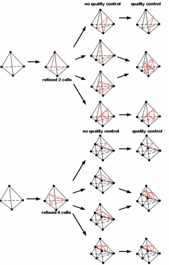
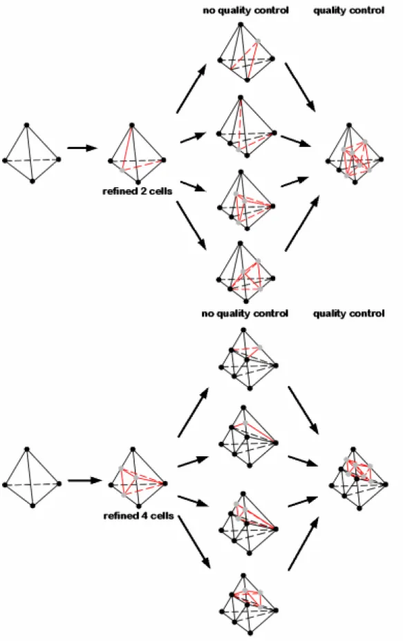
in a triangular cell, the cell must be divided into different way. However, for three-dimensional mesh, the division is more complex. The division would consider the number and position of the hanging nodes, to decide whether to add new nodes to obey the refinement rules. There are three results. One is to divide into eight child cells. Another is to divide into four child cells. The other is to divide into two child cells. The detail refinement rules are be show in Fig2.7.

A problem associated with repeated adaptive mesh refinement (AMR) operations.

Then, most mesh smoothing schemes tend to change the structure of a given mesh to achieve the “smoothing effect” (a better aspect ratio) by rearranging nodes in the mesh. The change made by a smoothing scheme, however, could modify the desired distribution of element density produced by AMR procedure, and the cost of performing a global mesh smoothing could be high. Alternatively, it is possible to prevent, or slow down, the degradation of cell quality during a repeated adaptive refinement process. The cell quality control scheme we have applied classifies element based on how they will be refined. This allows us to avoid creating elements with poor aspect ratios during the refinement. After identifying those elements, we can refine them with a better refinement by contrast.

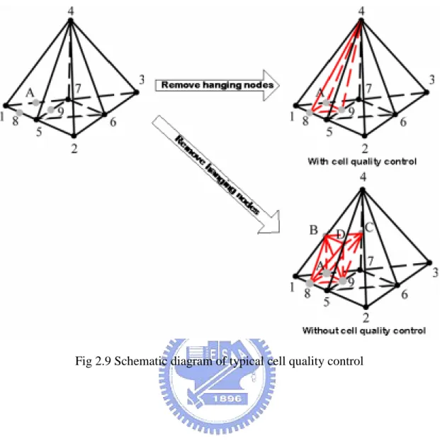
Detail rules are shown in Fig2.8. For example, Fig2.9 shows a typical cell

(1-2-3-4). Because it is affecting by other cell, it has hanging nodes (8, 9, A). In order to handle hanging nodes, we connect nodes (8, 9, A) to node 4. But the aspect ratios of typical cells (1-4-8-A, 5-4-8-9 and 7-4-9-A) will be worse. However, if we add three nodes (B, C and D), and connect them with other nodes. Those eight child typical cells (4-B-C-D, 1-8-A-B, 5-8-9-D, 7-9-A-C, 8-9-A-B, 8-9-B-D, 9-A-B-C and 9-B-C-D) would have better aspect ratios.

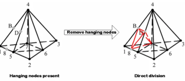
However in some cases, previous developed cell-quality-control would not be

effective that is shown in Fig2.10. For example, as showed in Fig2.11. At this

situation, after the last refinement there are four child cells. But at this refinement, there are three hanging nodes appear on edges (8, B, D). While cells are divided, it will be divided to four child cells. And these four child cells will not get worse aspect ratios. And, it would get better aspect ratios. So cell-quality-control will allow this

division and not to affect it.

If the boundaries of the computational domain are not straight, it is not sufficient to place the new node in the midway of the edge of the face of the parent cell. If this is done, it would dual to a rough piecewise representation of the original geometry results. What must be done is to move the new node location onto the real boundary contour surface. In the current implementation, it is assumed that the boundaries can be represented in parametric format. Specific neighbor identifiers are assigned to these non-straight boundary cells to distinguish from straight boundary cells. Whenever the boundary cells, which require mesh refinement, are identified as a non-straight boundary cell, the corresponding parametric function representing the surface contour are called in for mesh refinement to locate the correct node positions along the parametric surface.

2-7.3 Procedures of Parallel Mesh Refinement

Fig2.12 illustrates the flow chart of parallel adaptive mesh refinement (PAMR).

Details are described step in the followings. 1. Set up initial grids and input data.

2. Initialize MPI and synchronize all processors to prepare for parallel computation.

3. Read grid and relative cell data, and distribute them to every processor at the same time.

4. Find and record the cells which need to be refined, based on the refinement criterion calculated from the other module.

5. If there is no cell required to be required, stop the module. Otherwise, go to next step.

6. Add new nodes to cells based on the module I., which is described in detail later. In this step, communications among processors are required.

7. Renumber all new added nodes in this step to “unify” the node numberings for all processors. Note that the node numberings for all original nodes are kept the same as those before refinement. In this step, communications among processors are required.

8. Update connectivity-related data to new child and old parent cells.

9. Build up new neighbor identifier array. Communication among processors is required in this step.

10. Decide if it reaches the preset maximum number of refinement. If it does, then go to next step, otherwise return to step 4.

11. Synchronize all processors.

12. Host gathers all data and output the data at the same time.

In addition, all modules (I-IV in Fig2.12) in the core of the PAMR are explained in detail as follows.

Module I. Add nodes on cell edges (Fig2.13):

I-1. Add new nodes on all edges of “isotropic” cells that require refinement. These cells are called “isotropic” cells since it is refined from one cell to eight smaller cells.

I-2. Add new nodes to “anisotropic” cells, which may require further treatment in the following steps, if hanging nodes exits in these cells... Note that these cells are called “anisotropic” since they are not those cells originally require “isotropic” mesh refinement.

I-3. Communicate the hanging-node data to corresponding neighboring processors if the hanging nodes are located at the IPB (Interface

Processor Boundary). If hanging-node data are received from other processors in this stage, then go back to Step I-2 for updating the node data. If there is no hanging-node data received at this stage, then move on to the next step.I-4. Remove hanging nodes based on refinement rules, if need to add new nodes go to I-2. If all cells obey the rules without to affect them, it mean all new nodes are be added.

I-4 . Remove hanging nodes based on Hanging-node Removal rules. Go to Step I-2 to add new nodes if some more nodes addition is required. If there is no more node addition required, then ends this module execution.

Module II. Renumber added nodes:

II-1. Add up the number of the new added nodes in each processor, excluding those on the IPB.

II-2. Communicate this number to all processors. These are used to add up the total number of added nodes in the interior of all processors.

II-3. Renumber those added nodes in the interior of the processor according to results from Step-II-2.

II-4. Communicate data of added nodes on IPBs among all processors. II-5. Renumber the added nodes on IPBs on all processors.

Module III. Update connectivity data:

Form all new cells and define the new connectivity data for all cells.

Module IV. Build neighbor identifier array:

IV-1. Reset the neighbor identifier array.

IV-2. Rebuild the neighbor identifier array for all the cells based on the new connectivity data. Note that those nbr information on faces of

the cells on the IPBs are not rebuilt and require further treatment in the next step.

IV-3. Record the neighbor identifier arrays that are not built in Step-IV-2, which the neighbor of the interested cell locates in the neighboring processor.

IV-4. Broadcast all the recorded data in Step-IV-3 to all processors.

IV-5. Build the nbr information on the IPBs, considering the overall connectivity data structure.

2-8 Coupling Procedures of Parallel P-B Equation Solver with PAMR

2-8.1 Refinement Parameter and Criteria

All mesh need some means to detect the requirement of local mesh refinement to better capture the variations EDL fields and hence to obtain more accurate numerical solutions. This also applies to parallel Poisson-Boltzmann solver. It is important for the refinement parameters to detect a variety of EDL. In literature, the electric field usually to be adopted as the refinement parameter. The electric field is the potential gradient. We use the electric field as the refinement parameter in parallel Poisson-Boltzmann solver.

To use the electric field value as a refinement parameter, a local electric field can be defined as

Ψ −∇ =

E [2-36]

Where Ψ is the local cell potential. When the mesh refinement module is

initiated, local cell electric field value will be read in, and take compare with other cells around local cell. If the variation of electric field value between local cell and surroundings cell is more then preset value. We will give a symbol to refine both local

cell and surroundings cell. If not, we do not refine these cells.

2-8.2 Parallel Poisson-Boltzmann Solver with Mesh Refinement In Fig2.14, it shows couple PPB-PAMR method.

In summary, the following steps describe the mesh refinement:

1. Setup initial grids and input data.

2. Process PPB computation to get initial results.

3. Compute the refinement parameters in each cell.

4. Refine all the cells which are need to.

5. Create and update the grids data and input data.

6. Using the new grid data and input data to run PPB, to get new results.

7. Return to (4) if the accumulated adaptation levels are less than preset

maximum value.

8. If the accumulated refinement levels are greater than the preset value or no

mesh refinement is required. Stop the refinement mesh procedure.

9. Using the finial grids and input data to run PPB, and finish the all

Chapter 3 Results and Discussion

3-1 Code Verifications

To ensure the accuracy of the EDL potential distribution, the numerical results are also compared along with the analytical results. For the small electrostatic potential, Eq. [2-6] can be approximated by the first terms in a Taylor series. In the literature, this is call the Debye-Huckel linear approximation. This approximation is valid only for small values of electrostatic potentialψ . In this section, we will

compare our numerical results with the Debye-Huckel approximation and Tuinier’s [7]

approximate solution.

3.1-1 Potential Around a Sphere

Fig 3.1 shows the numerical model for the sphere, the dimensionless electrostatic

potential of the sphere surface is chosen to be constant potential. The Neumann boundary conditions are implied on the other boundaries of the domain. And in this case, the normalized radius a is chosen to be 5.

The Debye-Huckel linear approximation for sphere can defined as

( )

( )

x x a a x sp  −      + Ψ = Ψ 0 exp [3-1]

Where the sub “sp” refers to sphere, and a is normalized radius.

The approximate solution which proposed by Tuinier [7] is:

( )

_{( )}

( )

_      − − − +       + = Ψ x t x t x a a x sp exp 1 exp 1 ln 2 0 0 1 , [3-2] Where t is defined as 0       Ψ = 4 tanh 0 0 t [3-3]

kind of different results, are nearly all the same at smallΨ0 =1. Cleary, our PB solver

has certain accuracy. In Fig 3.3 we apply Ψ₀ =5at sphere surface. We can observe

form the figures; there is a very steep decrease in the numerical results, while the Debye-Huckel approximation predicts a more gradual decay of the potential. And we also can discover Tuinier’s approximate solution slightly under predicts the numerical results.

In Fig 3.4, we discuss the convergence situation between different initial guess. We use Debye-Huckel and Tuinier’s approximation to be initial guess, and compared with zero. Cleary, using Tuinier’s approximation to be initial guess has a good convergence situation; the Monotone sequence converges within two hundred iterations.

3.1-2 Potential Around a Cylinder

For cylindrical geometry, we do the same thing with sphere. Fig 3.5 is the

numerical model for the cylinder. We also chose cylinder surface to allow Dirichlet boundary, the other surface is Neumann boundary conditions.

The Debye-Huckel linear approximation for cylindrical can defined as

( )

(

)

) ( 0 0 0 a K a x K x cy + Ψ = Ψ [3-4]

Where the sub “cy” refers to cylinder and K is the zeroth-order modified 0

Bessel function of the second kind.

And the approximate solution for cylinder which proposed by Tuinier [7] is:

( )

_{( ) ( )}

(

)

( )

_{( )}

_      − − − + − + = Ψ x t x t x a K a x K x cy exp 1 exp 1 ln exp 2 0 0 0 0 1 , [3-5]

sphere. Debye-Huckel approximation also has wrong potential distribution at largeΨ.

3-2 Simulation of Two Interacting Identical Particles Coupled with PAMR

The problem deals with two identical colloidal particles immersed in electricity

neutral electrolyte. It was studied in several works [2, 3, 5, and 6] and can server as a

test. The numerical model is shown in Fig 3.8 We let segment AB to be half the

separation distance which is call h, surface CD and DE are assumed the infinite of

the electrolyte, surface BC represents a midplane for the problems with two particles.

In this case, the force of interaction of two particles of the radiusa=5and the

separation distanceh=0.5. The constant potential Ψ on the surfaces of both 0

particles is equal to 2.0. The Neumann boundary conditions are implied on the other boundary conditions of the numerical model.

The force of the interaction can be calculated by Eq. [2-23]. Here we will take integration over the surfaces of the particle.

In the Table 3-1 we can see the results in every refinement step; we can see the force at step 4 and step5 are almost the same. We speculate the mesh has become optimal at step 5. Fig 3.9 to Fig 3.14 is the mesh distribution for every refinement step, and Fig 3.15 is the potential distribution at final step.

It is ensured that the results shown in this article are independent of finite element mesh. The results obtained from different steps of the parallel adaptive mesh refinement are show in Table 3-1. From this table, it is clear that as we refine the mesh, the scaled of the force of the interaction obtained from the numerical solution of the Poisson-Boltzmann equation convergence toward a fixed value. After compares

with literature [6], we have almost the same results, but still have inaccuracy. The

interaction at the final step is 48.840. After compare with our result, we have 0.4

inaccuracy. At small separation distanceh=0.5 the force of the interaction is

repulsion.

3-3 Two Identical Particles in a Cylindrical Pore

In this section, we will computer experiments with a geometrically confined pair of spheres concern the phenomenon of long-range electrostatic attraction between

particles of like change [4]. The long-range electrostatic interaction of two colloidal

particles confined in a cylindrical pore was studied in the present paper [3], we use the

same values of parameters and geometry, such as the 1:1 electrolyte, the potential on

surfaces of the sphere particlesΨ_s =3.0, the potential on the cylindrical pore

surfaceΨ_p =5.0, the radius of the particlesa=1.185, the sphere radius to pore radius

ratio 0.13. The numerical model is shown in Fig 3.8;in this case we let surface CD to

be the cylindrical pore surface.

The results of the calculations are shown in Table.3-3. Positive values for the

force F mean repulsion, negative mean attraction. We calculate four different _s

separation distances,h=0.5, 1, 3.5, 6, 8, respectively.

Fig 3.16 and Fig 3.17 shows the calculated potential distribution for the sphere

confined in a pore at separation distances h=0.5andh=6. Fig 3.18 and 3.19 shows

the potential along the midplane BC ath=6. We can see the potential along this plane

is almost decreasing at all distance, but after Z=3.4 the potential become increasing. After compares with literature, we also have almost the same results, but still have 1% inaccuracy.

Chapter 4

Future Work

4-1 Summary

In the chapter three, we deal with the two cases, one is two free identical particles, and other is two identical particles in a cylindrical pore. In order to make sure code validity, we use the same parameter in previously literature. All of the previously works are assumes the numerical model is symmetry and reduce to two-dimensional problem. But the calculation of the interaction between two spheres

closed to a planar wall [4] requires a full three-dimensional problem. Assume the

problem to two-dimensional may have some uncertain. We develop this three-dimensional Poisson-Boltzmann equation just can to deal with this troublesome problem.

In the propose study, we can obtain the parallel Poisson-Boltzmann equation coupled with PAMR is very useful and convenience. It can be more closed to real situation at colloidal systems.

4-2 Recommendations for Future Work

In this propose study, we meet two difficulties, one is the convergence rate too slow, the other is refinement level can not over than five. We can use fine initial guess to overcome the convergence rate problem, but the cost of the refinement computation, we can not overcome directly. But there still have some way to overcome this situation, we can use the high order mesh and coupled different mesh such as hexahedral cell and pyramid. If we can use high order mesh to capture the EDL potential distribution, we can reduce the inaccuracy without large computationally cost.

References

[1] D.J. Shaw, Electrophoresis, Academic Press, New York, (1969)

[2] W.R. Bowen, A.O. Sharif, “Adaptive Finite-Element Solution of Nonlinear Poisson-Boltzmann Equation: A Charged Apherical Particle at Various Distances from a Charged Cylindrical Pore in a Charged Planar Surface” J. Colloid Interface Sci. 187(1997)

[3] W.R. Bowen, A.O. Sharif, “ Long-range electrostatic attraction between like-charge spheres in a charged pore” Nature 385 (1998) 663

[4] A.E. Larsen, D.G. Grier, “Like-charge attractions in metastable colloidal crystallites” Nature 385 (1997) 230

[5] P.E. Dyshlovenko, “Adaptive Mesh Enrichment for the Poisson-Boltzmann Equation” J. Comp. Phs 172 (2001) 198

[6] P.E. Dyshlovenko, “Adaptive numerical method for Poisson-Boltzmann equation and its application” CPC. 147 (2002) 335-338

[7] R. Tuinier, “ Approximate solutions to Poisson-Boltzmann equation in spherical and cylindrical geometry” J. Colloid Interface Sci 258 (2003) 45-49

[8] Prodip K. Das, Subir Bhattacharjee, “Finite element estimation of electrostatic double layer interaction between colloidal particles inside a rough cylindrical capillary: effect of charging behavior” Colloids and Surfaces A 256 (2005) 91-103 [9] R. –C. Chen, Jinn-Liang Liu. “Monotone iterative methods for the adaptive finite

solution of semiconductor equation” J. of Computational and Applied Mathematics 159 (2003) 341-364

[10] Almasi, G. and A., G., “Highly Parallel Computing, Benjamin/Cummings, Red-Wood city, CA,1989

Schemes on The Efficiency of Parallel Conjugate Gradient Iterative Methods for Finite Element Analysis” (2002) Graduate School of Clemeson University

[12] Yuan-Wen Jeng , NCTU MUST, ‘’Parallel Implementation of Three-dimensional Unstructured Mesh Refinement in the Direct Simulation Monte Carlo Method’ [13] Kuo, Chia-Hao, "The Direct Simulation Monte Carlo Method Using

Unstructured Adaptive Mesh and Its Applications,", MS Thesis, NCTU, Hsinchu, Taiwan 29, Jun., 2000.

[14] Wu, Fu-Yuan, "The Three-Dimensional Direct Simulation Monte Carlo Method Using Unstructured Adaptive Mesh and It Applications", MS Thesis, NCTU, Hsinchu, Taiwan , July., 2002.

[15] S. Levine, J.R. Marriot, G. Neale, N. Epstein. J. Colloid Interface Sci. 52 (1) (1975) 136-149

[16] S. Levine, G.M. Bell, Discuss. Faraday Soc. 42(1966) 69 [17] E. Bresler. J. Colloid Interface Sci. 118 (2) (1987) 326 [18] P.L. Levine, J. Colloid Interface Sci. 51(1975) 72

[19] T.A.R. Strauss, H.K. Bowen, J. Colloid Interface Sci. 118(2) (1987) 326 [20] H.K. Bowen, J. Colloid Interface Sci. 173 (1995) 388-395

[21] G.M. Mala, D. Li, C. Yang, ‘’Electrical double layer potential distribution in a rectangular micro channel,’’ Int. J. Heat Fluid Flow, (1997).

[22] Patankar, N. A., and Hu, H. H., ‘’Numerical Simulation of Electroosmotic Flow,’’ Anal. Chem. 70, 1870 (1998)

[23] Arulanandam, S., and Li, D., ‘’Liquid transport in rectangular microchannels by electroosmotic pumping,’’ Colloids and Sufaces A: Physicochemical and Engineering Aspects, 161, 89-102 (2000).

Microchannel,”J. Colloid Interface Sci., 244, 173-179, (2001).

[25] J. Yang, L. M. Fu, and Y. -C. Lin ‘’Electroosmotic Flow in Microchannels,’’ J. Colloid Interface Sci. 239, 98-105 (2001).

[26] H.A. Stone, A.D. Stroock, and A. Ajdari, Annu. ‘’Engineering Flows in small devices,’’ Rev. Fluid Mech. 36:381-411 (2004)

[27] R. -C. Chen, Jinn-Liang Liu. ‘’Monotone iterative methods for the adaptive finite

element solution of semiconductor equations,’’ J. of Computational and Applied Mathematics 159 (2003) 341–364

[28] Yiming Li, ‘’A parallel monotone iterative method for the numerical solution of multi-dimensional semiconductor Poisson equation,’’ Computer Physics Communications 153 (2003) 359–372

[29] R.J. Hunter Zeta Potential in Colloid Science: Principles and Applications, Academic Press, New York, (1981)

[30] H. J. Keh, and H. C. Tseng, J. Colloid Interface Sci. 242, 450-459, (2001) [31] J. Yang, and D. Y. Kwok, J. colloid Interface Sci., 260, 225-233, (2003) [32] C. C. Chang, and R. J. Yang, J. Micromech. Microeng., 14, 550-558, (2004) [33] Kuo-Hsien Hsu, NCTU MUST ‘’Three-dimensional parallelize Poisson slover’’ [34] W.B. Russel, D.A. Saville, W.R. Schowalter, Colloidal Dispersions, Cambridge

Table

Table3-1: Steps of the adaptive process:

Refinement level

Number of nodes Number of elements Force of

interaction(Fs) 0 924 3821 20.9924 1 3045 14305 34.6570 2 18253 96638 40.4853 3 132477 747048 44.0112 4 187732 1049734 48.0722 5 213224 1190741 48.4066

Table3-2: Steps of the adaptive process for previously literature [6]

Refinement level

Number of elements Force of interaction(Fs)

0 946 36.518 1 1992 43.716 2 4466 46.596 3 7642 47.597 4 11314 48.472 5 13525 48.630 6 15187 48.862 7 15477 48.826 8 15541 48.840 9 15555 48.843 10 15578 48.841 11 15588 48.840

Table3-3: The interaction forces of two particles in a cylinder pore at different separation distance.

Separation Distance(h) 0.5 1 3.5 6 8

Force of interaction(Fs) 26 13 -0.7 -4.7 0.9

Figure