Fuzzy control stabilization with applications to motorcycle control

836 IEEE TRANSACTIONS ON SYSTEMS, MAN, AND CYBERNETICS-PART B: CYBERNETICS, VOL. 26, NO. 6, DECEMBER 1996

ntrol Stabilization

wi

plications to Motorcvcle

J

Con

J. C. Wu and T. S

Abstract- This study develops fuzzy control that is designed with sliding modes to achieve stability of the fuzzy controller. Fuzzy control is formulated in the form of variable structure system (VSS) control. In contrast to previous works in which Lyapunov functions are used to examine the stability, the current study investigates the stability of fuzzy control from the view- points of differential geometric methods and the sliding mode theory. Best values for parameters in fuzzy control rules are determined with the aid of sliding modes. In order to improve control performance, a tuning algorithm is executed to adjust parameters for dealing with uncertainties and disturbances. Both computer simulations and experiments with regard to an inverted pendulum hinged to a rotating disk are carried out to validate the proposed method. This apparatus can to some extent represent cornering motion of a motorcycle on which a rider leans to main- tain stability. Effects of rider’s leaning angle on both stability and handling control are examined according to Bode plots.

I. INTRODUCTION

UZZY control research based on the fuzzy set theory [29] was initiated by Mamdani [19]. Fuzzy control is a direct method for controlling nonlinear ill-defined systems whose mathematical models are not exactly known. A fuzzy

controller is endowed with control rules that are constructed based on heuristic control of experienced human operators. Braae and Rutherford [l] proposed both algebraic model and linguistic model for fuzzy control. The algebraic model cannot deal directly with rules of fuzzy controller. Harris and Moore. [8] extended the linguistic approach to phase planes. They proposed a graphical analysis tool for considering overall system Performance. Johansen [ 121 carried out stability and performance analysis of a multi-input multi-output (MIMO) fuzzy model based control system. Wang [28] proposed an adaptive fuzzy system, in which a training algorithm adjusts parameters of fuzzy systems using numerical input-output pairs.

Although fuzzy control has been implemented in many industrial applications, there are few systematic procedures available for analysis and design of fuzzy control. Kiszka et al., [14] proposed the notion of energy for fuzzy relations to investigate local stability of fuzzy systems. However, the fuzzy relations describing the fuzzy system were exactly known, which contradict the main feature of fuzzy control. Langari and Tomizuka [15] proposed a method for the sta- Manuscript received August 21, 1994; revised September 3, 1995. This work was supported by the National Science Council, Taiwan, R.O.C., under Grant NSC84-2212-E009-004.

The authors are with the Department of Mechanical Engineering, Na- tional Chiao Tung University, Hsinchu 30010, Taiwan, R.O.C. (e-mail: tsliu @cc.nctu.edu.tw).

Publisher Item Identifier S 1083-4419(96)05395-2.

Liu, Member, IEEE

bility analysis of fuzzy control systems, in which Lyapunov’s direct method provided sufficient conditions for the stability. However, it is difficult to find out a Lyapunov function for higher-order systems. Lin and Kung [I61 proposed a fuzzy- sliding mode controller (FSC) that improved variable structure system (VSS) control with the aid of fuzzy control. Kawaji and Matsunaga [ 131 proposed, based on the VSS control, a method of generating fuzzy rules for servomotors. They determined linguistic values in fuzzy control rules and chose the best linguistic value based on both experience and trial and error. In contrast to [13], [15], and [16], the current study inves-

tigates the stability of fuzzy control from the viewpoints of differential geometric methods and the sliding mode theory, in which fuzzy control is formulated to become a class of VSS control. With the aid of sliding modes, it provides an effective design method for fuzzy control to ensure stability. The sliding mode optimization is employed to obtain the optimal switching function that minimizes a cost function. To improve control performance, a tuning algorithm is executed to adjust parameters in fuzzy rules for dealing with uncer- tainties and disturbances. To validate the proposed method, an experimental apparatus is designed and conducted in which an inverted pendulum is hinged to a rotating disk. Both computer simulations and experiments are carried out.

In this study, Section I1 describes definitions and assump- tions and then formulates fuzzy control. Section I11 presents the differential geometric method. The salient features in the sliding mode theory using the differential geometric method are described in Section IV. In Section V, fuzzy control rules are enacted with the aid of sliding modes and the stability is examined from the viewpoint of the differential geometric method. Section VI describes a case study to validate the proposed method.

11. FUZZY CONTROL A. Dejinitions and Assumptions

Several assumptions that facilitate formulation of fuzzy control in this study are described in the following:

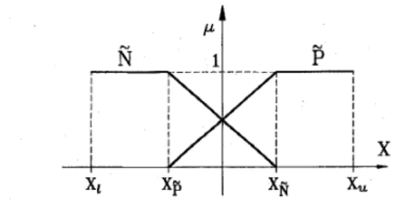
Assumption I : Let X be a universe. and N are fuzzy subsets whose membership functions are continuous but not differentiable mappings p: X + [0,1]. Define p p ( z ) and P N ( X ) as

WU AND LIN FUZZY CONTROL STABILIZATION WITH APPLICATIONS 837

Fig. 1. Membership functions of input variables.

where xu and x1 denote the upper and lower bounds in the universe, respectively. P and N are shown in Fig. 1, in which they form fuzzy partitions of a closed bounded region. Both P and

N

are normal, i.e., supz p p ( x ) = supz p f i ( x ) = 1,x E

[ X I , xu]. Moreover, for each x E [ x i , x u ]

P P ( 4

+

P N ( 4 = 1. ( 2 ) Assumption 2: Let A =

{ A j }

and

B

= {&} be collections of fuzzy subsets over E

c

X and EC

c

X , respectively. E

and EC denote the bounded universe for error e and error rate P: where P: = (ek - e k - l ) / T . This study assumes that each

of A and

B

contains only two fuzzy subsets as described in Assumption 1. According to (2), for any e E E and P: E EC

3 2

( 3 )

Assumption 3: Let U

c

X be a bounded universe for control input U . The combination of fuzzy control rules R, defined on E x EC x U, is expressed as the union of four individual rules; i.e.,

(4)

set of control input U can be expressed by, in terms of input values e0 and 60 .

where @ denotes the union operator, 0 the algebraic product operator, o the composition operator, and C,, i = 1,

. . .

,4 are fuzzy singletons. In this study, the algebraic product instead of the minimum operator is employed and results in interactivity among elements in (6). Let wj,l = p i , (eo) @ pfil (eo) denote rule strength of (5). Since Ej,l w3,1 = 1 from ( 3 ) , under the center of gravity method for defuzzification, the crisp value U can be written as

(7) where u3,1 is defined in (5). Since both wj,l and uj,i in (7) are continuous functions of eo and

eo,

U is a continuous and nonlinear function of eo and e o , i.e., fuzzy control is essentially a class of nonlinear control.

To gain insight into the relationship between fuzzy control and VSS control, the phase plane of e and 6 can be divided

into nine operating regions as depicted in Fig. 2(a), which accounts for Region 1: e

5

x p , 8

2

x f i Region 2: x p

<

e

<

x f i , 8 2 x f i Region 3: e 2 xfi,P: 2 x f i Region 4: e

5

x p ,

x p

<

P:

<

x f i Region 5: x p

<

e

<

x f i , x p

<

P:

<

x f i Region 6: e 2. x f i , x p

<

e

<

x f i Region 7: e

5 x p , 5 x p

Fuzzy control rules [26] containing two input variables e and

i: can be written as

Region 8: Region 9:

x p

<

e

<

x f i , 1

5 x p

e 2 x f i , &

5

x p Rj,1: If e is A3 and 1 is

B1

then uj,l =pbe

+

p2i: + p i

e E E , e E EC,u3,1 E U , i = 1

,

... ,4

_{( 5 )}

where p b , p ; , and

p i

denote parameters of linear dependence between nonfuzzy values of input variables and control input for the i-th fuzzy rule. The fuzzy controller contains four control rules since only two fuzzy subsets

P

and N are defined for each of E and EC as described in Assumption 2. This study employs fuzzy rules proposed by Takagi and Sugeno [26] to reduce the number of fuzzy subsets and fuzzy rules. By adjusting crisp values p j in ( 5 ) , via sliding modes in the current study, fuzzy rules can effectively correlate fuzzy subsets so that a multivariable and complex system is tractable. B. Formulation

Fuzzy sets provide a useful foundation to handle human knowledge pertaining to a real world problem and contribute to the notation of fuzzy control. The formulation for fuzzy control is described in the following. Given crisp input values eo and eo, assume that input values can be treated as fuzzy

singletons Go and

ko.

It follows from (4) and (5) that the fuzzy

The input variables e and P: in fuzzy rules are scaled based on measured and calculated values. This study assumes x p = - 2 and x~ = 2. The values of

xg,

and x f i are associated with scaling factors. As long as scaling factors are determined, values of x p and x f i can be obtained, and vice versa. The effect of scaling factors on control performance was investigated in [22]. Increasing scaling factors renders control performance more sensitive during the steady state response whereas less sensitive during the transient response. The upper bound, at which the system is too sensitive to converge, and the lower bound, at which the rise time and steady state error are too large to exhibit poor transient performance, have to be determined in order to choose scaling factors. Equation (7) in nine respective regions can be written as

OLw

+

H.O.T. when ( e , E) lies in

I

Regions 2, 4, 5, 6, and 8 when ( e , 6) lies in Regions 1, 3 , 7, and 9 (8)

838 IEEE TRANSACTIONS ON SYSTEMS, MAN, AI YD CYBERNETICS-PART B: CYBERNETICS, VOL. 26, NO. 6, DECEMBER 1996

.B

111. DIFFERENTIAL GEOMETRIC METHOD

Differential geometric methods [lo], [25], [27] have been developed for analysis and design of nonlinear control systems. The differential geometric method is an effective means of dealing with a class of nonlinear systems

1 l L 1 3

Fig. 2.

mination of control actions based on partition planes.

(a) Nine partition planes of error ( e ) and error rate ( 6 ) . (b) Deter-

where 0; = [0,10,2fl,3] denotes the parameter vector of

Region m, the base vector w = [leRIT, and H.O.T. denotes higher-order terms. Fuzzy control entails different control inputs U over different regions as shown in (8). Specifically

3 811 =Pz, Ol2 O13 = Pi 1 1 1 fl31 = P 2 , 032 P o , 033 Pi 4 071 = P i , 072 = l$, 873 = Pi 091 092 =

Pi,

fl93 = P?. (9)

Each of f, m = 1,

. .

' 9 is a continuous and differentiable

function in terms of e and P.. However, U is continuous but not differentiable on lines e = x~ e = x f i P. = x p and P. = x f i . Control inputs U in these nine regions are shown in Fig. 2(b), in which FL and F N ~ denote linear and nonlinear functions, respectively. Control inputs obtained from Regions 1, 3, 7 , and 9 are in the form of linear functions since u3,z in ( 5 ) are linear functions and only one rule fires in each of these four regions. Hence, fuzzy control is similar to PD control in these four regions. Fuzzy control in essence resembles VSS control since control inputs U vary with divided regions on the phase plane as shown in (8). Therefore, fuzzy control can be treated as a class of VSS control. Besides, the lines e = x p , e = x f i , P. = x1; and @. = x f i that divide the phase plane can be regarded as switching lines.

However, there are two differences between fuzzy control and VSS control. First, VSS control is generally devised with a sliding mode whereas fuzzy control is not. Secondly, control inputs of VSS control often change discontinuously whenever the trajectory crosses switching lines, on which sliding modes occur. By contrast, the variation of control input U in (8) for fuzzy control is continuous and no sliding mode occurs on four switching lines.

where x is assumed to belong to an open set

Ox

of R", f and g are R"-valued mappings defined on Ox, and h is a real- valued function also defined on

Ox.

The right-hand side of (10) is a linear function of control input U . The system (10) with (1 1) is said to have relative degree 7 at a point 50 if not only L,L!h(x) = 0 for k

<

I; - 1 and 2 around 50 but also L,LT-lh(rco)

#

0. The relative degree 'f; of a linear system can be interpreted as the difference between the numbers of poles and zeros in its transfer function.

Suppose the system has relative degree 'f; at 50 and set

If I;

<

n, it is possible to find ( n - I;) functions

4~+1

(x),

. . ,

and &(x) such that

L , ~ , ( z ) = 0 for all T

+

1 5 i

5 n

and all 5 around 5 0 and the Jacobian matrix of the mapping

is nonsingular at xo. The mapping is sufficient to define a coordinate transformation z = @(x). As a result of this transformation, the system (10) with (1 1) can be written as

where

When the output y of the system is constrained to (become zero, the resulting equation

from (13) is called the zero dynamics of the system [lo]. If the system (14) is asymptotically stable at

E

= 0, i.e., it is minimum phase [ 2 ] , one can determine the control input U to asymptotically stabilize the system (13).

WU AND LIN: FUZZY CONTROL STABILIZATION WITH APPLICATIONS - Zl - - 0 1 0

. . .

0 i 2 0 0 1 ' ' e 0 27-2 0 0 0 **e 1 * . -- . 3 - 1 - -cl -cg -c3

. . .

-c7-1- 839 - - 21 -, 2 2 XT-2 -27-1 - IV. SLIDING MODE THEORY

The VSS with sliding mode was proposed and elaborated by Emelyanov [4] and Itkis [11]. The VSS control employs switching and discontinuous control inputs to drive a phase trajectory toward a prescribed hyperplane, and to force the phase trajectory sliding on the hyperplane. The specific feature of sliding mode is that under certain conditions it remains insensitive to external disturbances and plant uncertainties. By properly designing the switching function, the sliding mode of a VSS control can guarantee to be asymptotically stable [3]. A detailed survey can be found in [9].

This section presents a formulation of salient features in the sliding mode theory using the differential geometric method, as described in [23]. Consider a single-input nonlinear system represented by the form

x = A ( x , U) (15)

where x E Oz. The mapping A defined on

Ox

is assumed to be a linear function of U . Let s denote a smooth function s:

Ox

-+ R, with nonzero gradient ds. The set

(16) defines a locally ( n

-

1)-dimensional submanifold on

Ox

that is called switching manifold. The switching manifold is of a lower order than the given plane. Moreover, parameters of the switching manifold dominate the dynamic behavior of the system during sliding mode control. Sira-Ramirez [24] claimed that the system (15) with the output y = h ( x ) has locally relative degree F = 1 if and only if a sliding mode locally exists on h ( z ) = 0. A variable structure control law is defined as

(17)

U =

P+

U - w h e n s < O w h e n s > o

where U + and U - are assumed to be smooth functions of x and to satisfy U+ > U - without loss of generality. A sliding mode exists on S if

s

= {z E

ox,

s ( z ) = O}

and lim L A ( z , u - ) ~

>

0. s+-0

Equation (18) can be rewritten as, in terms of a Lyapunov quadratic function,

s

#

0.

The sliding mode motion is described by

s = 0 and B = L A ( ~ , ~ , , ) s = 0 (20) where ueq denotes an equivalent control. The existence of ueq is only a necessary but not sufficient condition for the existence of sliding mode. The necessary and sufficient condition for the existence of sliding modes is that U+

>

ueq

>

U - [23]. Let

&(z) denote a subspace of the tangent space TxOx on Oz, such that

(ds,

As(%))

= 0 (21)

where (., .) represents an inner product. It follows from (21) that A,(x) constitutes the null space of ds. According to (20) and (21), one can obtain A(z,ueq) E A,(z).

The sliding mode theory generally entails switching func- tions that are presented by lines on the phase plane. VSS

control is generally devised with the sliding mode theory. Although it can also be devised without a sliding mode, such a system would not possess the associated merits. The feature of VSS control is that the sliding mode occurs on the switching manifold and the system remains insensitive to external disturbances and plant uncertainties.

Accordingly, if all roots of s"-1+g-lsT~2+. . .+czs+cl = 0 lie in the left-half s-plane, where s denotes a Laplace operator, the sliding motion on hz(z) = 0 is stable subject to feedback control input.

For ease of formulation, it is assumed that x contains two terms, i.e., z E 0%

c

R2. Under uncertain conditions, in the phase plane (10) can be rewritten as

where z1 denotes error e and xz error rate

e.

It is assumed that both f ( z ) and g(z) contain uncertainty that is unknown but lies within a prescribed set 0.19. The switching function is defined as

840 IEEE TRANSACTIONS ON SYSTEMS, MAN, AND CYBERNETICS-PART B: CYBERNETICS, VOL. 26, NO. 6, DECEMBER 1996

where the slope

x

denotes a positive constant. In order to obtain the optimal value of

3,

the optimization of sliding mode is implemented in the following.

A. Optimal Sliding Modes

In this study, the optimal switching function is obtained from sliding mode optimization. It is desired to design a switching function for (24) such that in sliding modes the cost function is minimized. Define a cost function

B. Parameter Determination for Fuzzy Rules

Since the system (24) with y = s(z) has relative degree r = 1, a locally sliding mode exists on s(z) = 0. As a result of coordinate transformation z = [s(z) x1IT, the system (24) becomes - i 1 = b ( z )

+

a ( z ) u (33) (34) 00

I = l

x T Q x d t where

(26) Apparently, the sliding dynamics ZZ = -322 for

>

0 repre- sents a minimum phase and the sliding motion on z1 = s ( z ) = 0 is asymptotically stable subject to feedback control input. To carry out feedback linearization, substituting a control input

Suppose a switching function is defined as

into (33) yields

(36) s = so(z1)

+

2 2 = 0

Zl

= -QZ1, a:>o where so(z1) is a function of 51, i.e., it may be nonlinear. It is

desired to determine s g ( z 1 ) such that I reaches its minimum for motion on s = 0. Introduce a new variable 'U defined as

which implies limtim z l ( t ) = 0 that is the desired result for sliding modes. If a Lyapunov function is prescribed as V = 212, (19) yields

From (27), rewrite (24) and (26) to become (37)

For the system (28) with the cost function (29), the optimal vector 322 can be derived as

where P E R is the solution of the Riccati equation

Since Q11, Q 1 2 , Q z l , and Q 2 2 are scalars for the system (24),

(31) is a second order algebraic equation in P. The solution of (31) reads P = - & l a

+

d-.

Substituting P into (30) and comparing (30) with (25) yields the optimal

x;

i.e.,

I

Accordingly, the sliding mode exists on z1 = s(z) = 0. Unlike VSS control that provides discontinuous control input, fuzzy control in essence exerts continuous control input. Hence, the present study uses (35) and (36) to design a con- troller such that the phase trajectory can approach switching lines asymptotically. VSS control uses discontinuous control inputs U+ and U - in (17), which often result in chattering in sliding modes. To avoid chattering that is present in VSS control, the parameter a in (36) is time-varying and acts like a boundary layer that has been proposed by Slotine and Li

[ 2 5 ] . Further, in a manner similar to Padeh and Tomizuka

[21], the present method facilitates fast convergence and good robustness in addition to asymptotic stability.

To determine twelve parameters p: , i = 1,

.

3

. ,4,

j = 0, 1 , 2

in four fuzzy rules, Regions 1, 3, 7 , and 9, as shown in Fig. 2, are considered since O m l , O m 2 , and Brh3, m = 1 , 3 , 7 , 9 are equal to twelve parameters p3s as shown in (9). In addition, control inputs in these four regions are expressed by linear functions, as shown in (8), which facilitate determining parameters. Equation (8) is used to approximate U* in (35), which is feedback control based on sliding modes, i.e.,

Apparently, optimal the matrix

&.

only depends on diagonal elements of Due to (9), O m , m = 1 , 3 , 7 , 9 consists of p i . Consequently, these twelve parameters can be determined by (38).

WU AND LIN: FUZZY CONTROL STABILIZATION WITH APPLICATIONS 841

+

Y

Both nonlinear terms b ( x ) and U(X) in (33) are not ex-

Tuning Algorithm

and T denotes the sampling time. The main feature of the tuning algorithm represented by (40) and (41) lies in that its tuning is on the basis of switching function values instead of errors, so as to on-line adjust parameters in fuzzy rules. It is desired that the tuning algorithm ensures the convergence of

s k . Substituting uk and uk-' in (39) into (41) yields g-'(z">r.;+l - f 2 ( 2 ' ) ] - g-1(2'--')[5: - f2(xk-')] actly known due to the uncertainty of f and g in (24). The cancellation of nonlinear terms in (35) is not exact in conducting feedback linearization. This study employs

(43)

< 7

-

Substituting x$ = s k -

%I$

and 2;'' = sksl -

Ax:+'

from (42) into (43) yields

Plant

off-line design is used to handle model imprecision. Fig. 3

+

shows the block diagram of fuzzy control with the tuning

= [ f 2 ( 2 )

+

xx$+l] - s(2')s-1(2"-l)[f2(s~-1)

+ x.3.

(44)

Furthermore, since g ( x k ) LX g(z"') for small T I (44) be-

output

>

where @ $ ] @!]

@,

and @$ are calculated when a phase point (e',

ik)

is located in the second, first, third, and fourth quadrants, respectively.

In this study, both sliding mode theory and differential geo- metric method provide an analytical approach to investigating stability of fuzzy control. The differential geometric method provides existence conditions for sliding modes, as described in Section IV. The control input of fuzzy control is formulated in the form of VSS control (8), thereby fuzzy control is designed. Moreover, the stability analysis of fuzzy control designed with sliding modes is achieved from the differential geometric method. According to the differential geometric method, if the zero dynamics is minimum phase, fuzzy control can indeed lead to asymptotic stability [lo]. With the aid of sliding modes, parameters in fuzzy rules can be off-line determined by (38), for which asymptotic stability is ensured by (36) and (37). The on-line tuning algorithm, which adjusts the parameters using (47), can achieve asymptotic stability as long as (46) is satisfied.

VI. CASE STUDY A. System Model

A rider-motorcycle integrated system can be treated as a man-machine system. Although a motorcycle is statically unstable in nature, appropriate steering of the rider enables the motorcycle to stabilize during riding. To maintain stability, with respect to tire bottoms on the ground, the moment comes

S k + l - U l S k

+

a z s k - 1

=

[f2(,p)

-

f2(&1)l + x [ f l ( x k ) - f1(2k-1)] (45)

where a1 = 1 +g(sk))p(l

+

l / a T ) and a2 = g(zk)P/aT. Fu- ruta [6] presented that the stability is guaranteed if

<

s g .

842 IEEE TRANSACTIONS ON SYSTEMS, MAN, AND CYBERNETICS-PART B: CYBERNETICS, VOL 26, NO 6, DECEMBER 1996

arising from the gravity force must be equal to but opposite to the direction of the moment due to the centrifugal force during cornering. Liu and Wu [ 171 employed the fuzzy control method to investigate the performance of rider-motorcycle systems. Forouhar [5] proposed a feedback control scheme based on robust optimal control theory to improve the dynamic behavior of motorcycles

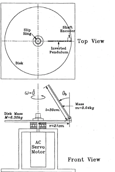
In this study, an inverted pendulum hinged to a rotating disk as shown in Fig. 4 represents cornering motion of a motorcycle on which a rider leans to maintain stability. This apparatus is designed in such a way that it can to some extent represent motion control involving the leaning angle of rider's body (represented by the inverted pendulum) and the banking speed of the motorcycle (represented by the disk). In a manner similar to the balance during motorcycle cornering, the inverted pendulum is not stable at any tilt angle unless both moments caused by the pendulum weight and the centrifugal force counteract each other. The inverted pendulum representing a rider's body in leaning motion is hinged to the rim of the rotating disk. The centrifugal force resulting from the rotating motion of the disk enables the inverted pendulum to rotate about the tangential direction of the disk. Disk rotating speeds that correspond to riding speeds of the motorcycle dominate the leaning motion of the inverted pendulum that corresponds to the rider's leaning motion. This study controls the tilting inverted pendulum to approach target angles using fuzzy control with the aid of sliding modes. It is desired to vary rotating speeds, so that the tilt angle can be controlled by the centrifugal force that arises from disk rotation.

The Hamiltonian formulation constructs the system model in terms of generalized coordinates and generalized momenta and thus results in a set of first-order equations of motion. Fur- thermore, solution trajectories for equations of motion derived by the Hamiltonian formulation form a phase space that lends itself to the qualitative description of the system behavior. To derive Hamilton's equations, generalized coordinates and generalized momenta are defined as

- -

Hamilton's equations [7] are accordingly written as

(49) where U denotes the generalized force, i.e., the torque of the motor, CO, and CO are respectively damping coefficients of the inverted pendulum and the disk to account for viscous damping at joints, and moments of inertia are formulated as

Ib = ;ml2 I M = i M r 2

+

m(r - $ 1 . sin Q b I 2 IC = m ~ ( r - + ~ . s i n ~ b ) c o s ~ b . (50) I I Disk Mass M=6.30ka

a

I

IServol

I I

I

I

IMotorl

I I

Top View

I I I

I I I

Front

I I I I r---J'

View

Fig 4 Schematic diagram of an inverted pendulum hinged to a rotating disk.

Neglecting generalized force and damping, i.e., U = 0 and Cob = CO = 0, (49) gives equilibrium points: p = O , Q b = 0, &7r, &27r,. . .

,

whereas 6' is arbitrary. If damping exists, as depicted in Fig. 5 , equilibrium points (n, 0), (37r, 0), etc. become stable nodes that account for the pendulum in the vertically downward direction.

B. Analysis Let

IC = [qT

PTIT

(51)

(49) yields

x = f(Z)

+

g(IC)u. (52)

The system is locally reachable [27] around ICO =

[e*

Gt 0 polT since the distribution A,(Ic~) = span{ad>g,0

5

z

5

3) has dimension 4, where Q b denotes the desired angle of inverted pendulum,

Fe

constant, and W the motor angular velocity at Ob =

8 b .

However, the system (52)

is not input-state linearizable [lo], i.e., there does not exist an output function ~ ( I c ) for which the system has relative degree r = 4 at 2 0 , since the distribution

AD

= span{g, a d f g , ad$g}

-

WU AND LIN FUZZY CONTROL STABILIZATION WITH APPLICATIONS 843

Letting z1 = z2 =

z3

= 0 in (54) and (53, the zero dynamics is expressed by

24 = ( e - ce)T(O, O,O)

+

U (56) where

Y(O,O, 0) =

F

r

-

1/2 sin 6'6

Due to constant $ b , ( e - Ce)r(O, 0,O) in (56) is a constant

value. Moreover, 2 4 = ex2

+

5 4 from (53) and 24 =

CO

+

1 ~ 0 from (48), (49), and (51). The internal dynamics

24

= ( c -

0 3.14 6.28

&(rad) Fig. 5. Phase planes of and p s , without control

is not involutive in the neighborhood of 20. Suppose the

output function is prescribed as

In this case, L,hl(z) = L , L f h l ( z ) = 0 and L,L'$l(z) =

- 2 4 ( 1 ~ ( 2 1 ) / I b I ~ ( 2 1 ) ) . The system has relative degree ?= =

3 if z4

#

0 and 5 1

#

( n

+

1/2)7r. This means that a locally

normal form can be found away from any point where 2 4 = 0

(corresponding to the motor at rest) and z1 = ( n

+

1/2)7r (corresponding to the pendulum that becomes horizontal).

- y = hl(z) = ~1 - 0 b .

To find the normal form, set

21 = (bl(2) = hl(z) = 51 - e b 5 3 I 6 2 2 =#J2(2) = L f h l ( Z ) = - 2 4 = 44(2) = c52

+

2 4 z3 =(b3(z) = L;hl(z) = (b3(21,23,24) (53) where c denotes a constant, together with its inverse transfor- mation

(54) The motor rotates counterclockwise from its top view since z4 in (54) is positive. In addition, x4 may also be equal to -IM(zI)$z~, 22, x g ) and hence the motor rotates clockwise.

Under this new coordinate z = (a(x), the system can be written as

C e ) ~ ( z l , 2 2 , xg)

+

U expressed in (55) accounts for the motor dynamics. If the internal dynamics is stable in the bounded- input bounded-output (BIBO) sense, the control system (55) can be stabilized [25]. However, it is not amenable to directly determining stability of the internal dynamics. Delineating the characteristics of zeros in transfer functions [lo], the zero dynamics (56) is hence employed to facilitate determining stability of the internal dynamics. The zero dynamics (56) is indeed minimum phase since an AC servo motor is operated in this study such that U in (56) implicitly contains the feedback control term -kzg where IC denotes a positive gain. Therefore, the system (55) can be stabilized by applying nonlinear control input U .

To carry out sliding mode control, the switching function for the system (55) can be specified as

It follows from (53) that

where c1 and e2 are constants. Equation (57) implies the assumption that z1,z2, and 23 and hence from ( 5 3 ) state variables 2 1 , z3, and 2 4 are available for measurement. Since

the system (55) with y = hz(z) has relative degree F = 1, a locally sliding mode exists on hz(z) = 0. The sliding motion on h 2 ( ~ ) = 0 is stable subject to feedback control input if both roots of s2

+

cas

+

c1 = 0 lie in the left-half s-plane.

Since the system (52) is not input-state linearizable, it is difficult to control four states z simultaneously by one- input only feedback linearization. Nevertheless, substituting

5 4 = I ~ ( z l ) y ( z l , z2,z3) in (54) into the second equation in (49) yields 6' = w = y ( q , 5 3 , 5 4 ) . That is, the motor angular

velocity w depends on the control of 6'b. It requires a larger w

to track a larger target angle of 6'6. This applies to motorcycle cornering in the sense that only a larger body lean of the rider can accomplish faster cornering motion. Since an AC servo motor is operated in this study, its resulting w variation being treated as accurate as desired, only the control of 6'b is considered in the following. Let x = [Ob - $b Pe,/IbIT and

U = ( p e / I ~ ) ' = w 2 , the system is described by

x = f(z)

+

g ( z ) u y = x 1

844 IEEE TRANSACTIONS ON SYSTEMS, MAN, AND CYBERNETICS-PART B. CYBERNETICS, VOL. 26, NO. 6, DECEMBER 1996

where

=

[-%I

p,:

.

The system (58) is locally reachable and input-state lineariz- able arou,-.. -CO = [OO]'. The switching function of the system can be expressed as

s(Z) = 1x1 f 5 2 = x ( # b - g b )

+

e b (59) where

1

denotes a positive constant. Since the system (58) with y = S(Z) has relative degree F = 1, a locally sliding mode exists on S(Z) = 0. Moreover, the sliding motion on S(Z) = 0 is stable subject to feedback control input since

x

\ is positive. Under new coordinate

x

= [s(z)

x1IT

the system

(58) is written as (60) (61) Zl = b(z)

+

a ( z ) u z 2 = 21 - Ax2 - where

defined as Q11 = 100 and Q22 = 1 and then the slope = 10 from (32). Adequate values of

a,P,

and T in (41) and (42) enable the tuning algorithm to converge. Note that g(z) in (58) is not constant since IC in (50) varies with 8 b . From (46) and g(z), bounds of a,P, and T that ensure convergence can be calculated. Substituting (62) and (63) into (35) gives

U* = bo

+

ble

+

b28

+

Higher order terms (65) where

mgl - mgl -

bo=-sinOb, IC b 1 = -cos&+aX

k!

Twelve parameters p:s in the consequences of four rules in (64) are determined and tuned by (38) and (47), respectively. For instance, to determine parameters p ; , p:, and p i in the second rule of (64), Region 9 depicted in Fig. 2 is considered since only in Region 9 the second rule is fired according to (8) and (9). From (64), control input in (60) in Region 9 is

U = w 2 = ( p i ) 2 +p&ie+p:pii:+Higher order terms. (66) For specified target angle

&,

= 20" and a = 10, using (66) to

mgl CO approximate (65), i.e., U M U * , three parameters in the second

rule in (64) are obtained as (62) b(z) = __ sin(x2 + e h )

+

(X

-

L ) ( x ~ - 1 x 2 ) 2 1 b I h and IC a(.) =

--.

2 I b -

From (61), the sliding dynamics Z2 = -Ax2 is a minimum phase since is positive.

C. Simulation Results

In this study, initial conditions are prescribed as: the inverted pendulum angle O b = 36", its angular velocity 8 6 = 0, and the motor angular velocity w = 0. The inverted pendulum is initially supported by a vertical strut such that

&,

can never exceed 36". Four cases are investigated in which Cases I and I1 are used to examine stability control whereas Cases 111 and IV are used to examine handling control. The target angles of the inverted pendulum in Cases I and I1 are 20" and lo", respectively. By contrast, the target angles in Cases I11 and IV are prescribed to change from 20" to 10" and from 10" to 20" at the fifth second, respectively. The present fuzzy control contains both coarse-tuning and fine-tuning controls. Since P (positive) and

fi

(negative) are denoted as fuzzy subsets for input variables as depicted in Fig. 1, four fuzzy rules can be written as, in the form of

(3,

IF e is

P

AND 1 is

P

THEN w = p ; . e + p i . & + p i IF e is

fi

AND & i s THEN w = p : , e + p ; .i: + p i IF e is

fi

AND i is

fi

THEN w = p t . e + p f . i: + p i (64) where error e denotes the current angle of the inverted pen- dulum minus the target angle and 8 the error rate. To obtain the optimal value of

1

in (59), the elements of Q in (26) are

IF e is

p

AND 1 is

#

THEN w e + p ; . i: + p z 2

p i = 34.13, pf = 1.132, p z = 4.74. (67)

It is noted that three values in (67) are obtained when e and

i: are not scaled. In order to specify scaling factors, the upper bound, at which the system is too sensitive to converge, and the lower bound, at which the rise time and steady state error are too large to exhibit poor transient performance, have to be determined. Let scaling factors for e and i: be 285.7 and 10, respectively, three parameters in the second rule are calculated as

(68) In a similar manner, considering Region 1 in Fig. 2 due to (8) and (9), three parameters of the third rule in (64) are calculated as

2

p , = 0.12, p: = 0.11, p ; = 4.74.

p ; = 0.12, p: = 0.11, p ; = 4.74. (69) Since the switching function (59) is located in the second and fourth quadrants due to

>

0, it passes through Regions 1 and 9 Hence, control inputs in Regions 1 and 9 are similar to the equivalent control U,* given in (20). By contrast, control inputs in Regions 3 and 7 are similar to U+ and U - expressed in (17), respectively. Due to (8) and (9), parameters of the first and fourth rules are determined by considering Regions 3 and 7 in Fig. 2, respectively. Since the existence condition of sliding modes is U+

>

ueq

>

U - [23], parameters of the first and fourth rules in (64) are

p: =0.12, p i = 0.11, p i = 4.90

p $ =0.12, p: = 0.11, p; = 4.58. (70) Parameter values expressed in (68)-(70) comprise 12 param- eters of four rules in (64).

WU AND LIN: FUZZY CONTROL STABILIZATION WITH APPLICATIONS 845

40 I I I I I I O I

-With Tuning

.e..- Without Tuning -

h

d?

\

10 - 0 I I I I I I I I I 0 2 4 6 8 10 Time ( 5 ) I I I 0 \ \ I -80

t

I I L \I I 0 10 20 30 40 (b) Fig. 6 .

and (b) phase trajectories for Cases I and 11.

Simulation results of (a) angular displacement of inverted pendulum

Fig. 6 shows simulation results for Cases I and 11. Sim-

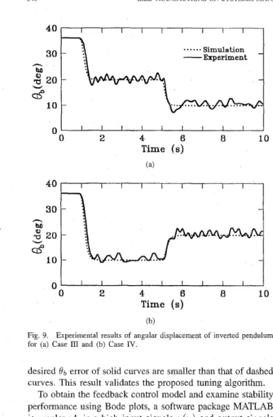
ulation results for Cases I11 and IV are shown in Fig. 9. The same control rules whereas parameters vary with target angles. To validate the tuning algorithm, bounded white noise is exerted from the 2nd to 10th seconds during excursion. It is seen in Fig. 6(a) that fuzzy control with the tuning algorithm can deal with disturbances. The phase trajectories shown in Fig. 6(b) initiate from O b = 36" and

&

= 0 for both cases. They approach switching lines asymptotically due to (36) but do not slide exactly on them. This is anticipated since the switching lines are the prescribed reference lines and control input for fuzzy control is continuous, as described in Section II.B, the sliding mode cannot be fulfilled perfectly. Besides, discrete-time VSS control can only achieve quasisliding modes according to [20].

D. Experimental Results

The schematic diagram of the experimental setup is shown in Fig. 7. A shaft encoder at the hinge of the inverted pen- dulum measures the tilt angle. An interface card transmits the position count to PC to carry out fuzzy control. The sampling time of PC command is lms. A motor driver receives control signals via the interface card, and enables instantaneous rotation motion of the AC servo motor. The initial angle of pendulum O b is 36" and the rotational velocity of the motor

w = 0.

Figs. 8 and 9 depict experimental results for four cases. Data is collected at a sample rate of 25 Hz. In contrast to simulation results, curve wiggle is present due to gear

Shaft Encoder Binary Counter Servo Motor Driver Interface

I

Card

1

6,

Interface

Fig. 7. Block diagram of experimental setup.

40

-

I I I I I I I I I

-

n W

crp

l o t

o t

I I I I I I I I I 0 2 4 6 8 10 Time (s) (a) 40 I I I I I I I I I _I 30

h

l o t

1

0 0 2 4 6 8 10 Time (3) (b) Fig. 8.

for (a) Case I; and (b) Case 11.

Experimental results of angular displacement of inverted pendulum

collision at backlash in the gearbox for the servo motor. The collision occurs whenever the motor undergoes large acceleration or deceleration. The collision hence belongs to random disturbances. For both cases in Fig. 8, relative to the

846 IEEE TRANSACTIONS ON SYSTEMS, MAN, AND CYBERNETICS-PART B: CYBERNETICS, VOL. 26, NO 6, DECEMBER 1996 40 I I I I I I I I I

...

Simulation

-

Experiment 10 0 - I I I I I I I I I 0 2 4 6 8 10 40 I I I I I I I I I n l I I I I I I I I I - 0 2 4 6 8 10 Time (5) (b) Fig. 9.

for (a) Case I11 and (b) Case IV.

Experimental results of angular displacement of inverted pendulum

desired O b error o f solid curves are smaller than that of dashed curves. This result validates the proposed tuning algorithm.

To obtain the feedback control model and examine stability performance using Bode plots, a software package MATLAB is employed, in which input signals u(n> and output signals y ( n ) are assumed to be related by a linear system [18], i.e.,

y(n) = G(')u(n)

+

~ ( n ) n = 1 , 2 , . . .

,

N where G(q ) denotes a transfer function, q a shift operator, and the disturbance v(n) can be described as filtered white noise. An ARX-model in system identification that implements the least square estimation method is used to estimate the system model based on collected input-output data. The ARX-model is written as

where k denotes the number of delays between input and output and

A(q) = 1

+

ulq-'+

.

+

unaqPna B(q) = bl

+

b2q-1 -I-.

. .

+

b n b q - n b + l .

Resulting from the estimated model (71), Bode plots are presented in Fig. 10, which shows Bode plots of O b versus the motor angular velocity w for Cases I and II. It can be seen from the phase angle plot that the system exhibits a minimum phase. Gain margins of both cases are very large. Case I (target angle 20" and Case I1 (target angle IO") yield phase margins of 85.7" and 54.7", respectively. The smaller target angle

0 e M a -60 U

2

8

-120 I I I I l i l l l I I I I l l l t l I I I I 1 1 1 1 1 0-1 1

oo

1

oi

1

oz

Frequency (rad/s)

Fig. 10. Bode plots in experiments for Cases I and 11.

results in larger phase lag. It is noted that compensating for larger phase lag requires more control effort. Corresponding to cornering motion of a rider-motorcycle system, the rider must bank at an adequate angle in order to maintain balance when the radius of the circular motion is constant. Therefore, a smaller leaning angle exhibits a poor stability control. On the other hand, handling controI is examined from Fig. 11, which shows Bode plots of O b versus the motor angular velocity w in the period of target angle change for Cases 111 and IV. Phase margins in Cases I11 and IV are 65.2" and 32", respectively. The phase lag in Case IV is larger than that in Case 111. From the viewpoint of a rider-motorcycle system undergoing rider's posture change, Fig. 11 demonstrates that it takes more handling control effort for a rider to increase than to decrease the leaning angle. Accordingly, stability control and handling control contradict each other. Trade-off between stability and handling control is thus needed for the motorcycle design

VII. CONCLUSIONS

This study has proposed a method for developing fuzzy control that is designed with sliding modes to ensure stability of the fuzzy controller. The stability has been investigated from the viewpoints of differential geometric methods and the sliding mode theory, in which fuzzy control has been formulated in the form of VSS control. The differential geo- metric method provides existence conditions for sliding modes. Sliding modes facilitate determining best values of parameters in fuzzy control rules. For the stability control, experiments demonstrate that the smaller the desired leaning angle of a rider is, the more difficult it is to maintain stability. For the handling control, it takes more handling control effort for a rider to increase than to decrease the leaning angle. Consequently,

WU AND LIN: FUZZY CONTROL STABILIZATION WITH APPLICATIONS 847

s

I-

Frequency (rad/s)

Fig. 11. Bode plots in experiments for Cases Ill and IV

stability control and handling control contradict each other. These results are consistent with human’s riding experience. Motorcycle design hence has to compromise between stability and handling performance.

REFERENCES

[ I ] M. Braae and D. A. Rutherford, “Theoretical and linguistic aspects of the fuzzy logic controller,” Automatica, vol. 15, pp. 553-577, 1979.

[2] C. I. Byrnes and A. Isidori, “A frequency domain philosophy for nonlinear systems with applications to stabilization and to adaptive control,” in Proc. 23rd IEEE Con$ Decision and Control, Las Vegas,

NV, 1984, pp. 1569-1573.

[3] C. M. Dorling and A. S. I. Zinober, “Two approaches to hyperplane design in multivariable variable structure control systems,” Int. J. Control, vol. 44, pp. 65-82, 1986.

[4] S. V. Emelyanov, Variable Structure Control Systems. Moscow: Nauka, 1967.

[SI F. A. Forouhar, “Robust stabilization of high-speed oscillations in single track vehicles by feedback control of gyroscopic moments of crank- shaft and engine inertia,” Ph.D. dissertation, University of California, Berkeley, 1992.

K. Furuta, “Sliding mode control of a discrete system,” Syst. Contr.

Lett., vol. 14, pp. 145-152, 1990.

H Goldstein, Classical Mechanics, 2nd ed. Reading, MA: Addison-

Wesley, 1980.

C. J. Harris and C. G. Moore, “Phase plane analysis tools for a class of fuzzy control systems,” in IEEE Int. Con$ Fuzzy Syst., San Diego,

J. Y. Hung, W. Gao, and J. C. Hung, “Variable structure control: a survey,” IEEE Trans. Ind. Electron., vol. 40, pp. 2-21, 1993.

A. Isidori, Nonlinear Control Systems: An Introduction, 2nd ed. New

York. Springer-Verlag, 1989.

U. It!&, Control Systems of Variable Structure. New York: Wilev,

CA, 1992, pp. 511-518.

[ 141 J. B. Kiszka, M. M. Gupta, and P. N. Nikiforuk, “Energetistic stability of fuzzy dynamic systems,” IEEE Trans. Syst., Man, Cybem., vol. SMC-15,

no. 6, pp. 783-792, 1985.

[IS] G. Langari and M. Tomizuka, “Stability of fuzzy linguistic control systems,” in Proc. 29th IEEE Coni Decision and Control, Honolulu,

HI, 1990, pp. 2185-2190.

[ 161 S. C. Lin and C. C. Kung, “Linguistic fuzzy-sliding mode controller,” in

Proc. I992 American Control Con$, Chicago, IL, 1992, pp. 1904-1905.

[17] T. S. Liu and J. C. Wu, “A model for a rider-motorcycle system using fuzzy control,” IEEE Trans. Syst., Man, Cybem., vol. 23, pp. 267-276,

1993.

[I81 L. Ljung, System Ident.$cation: Theory for The User. Englewood

Cliffs, NJ: Prentice-Hall, 1987.

[19] E. H. Mamdani, “Application of fuzzy algorithms for control of a simple dynamic plant,” in Proc. Inst. Electr. Eng., vol. 121, pp. 1585-1588,

[20] C. MilosavljeviO, “General conditions for the existence of a quasis- liding mode on the switching hyperplane in discrete variable structure systems,” Automat. Remote Control, vol. 46, pp. 307-314, 1985.

[21] R. Paden and M. Tomizuka, “Variable structure discrete time position control,” in ,Proc. American Control Confi, San Francisco, CA, 1993,

pp. 959-963.

[22] T. J. Procyk and E. H. Mamdani, “A linguistic self-organizing process controller,” Automatica, vol. 15, pp. 15-30, 1979.

[23] H. Sira-Ramirez, “Differential geometric methods in variable-structure control,” Inc. J. Control, vol. 48, no. 4, pp. 1359-1390, 1988. [24] -, “Nonlinear variable structure systems in sliding modes: the

general case,” IEEE Trans. Automat. Contr., vol. 34, no. 11, pp. 1186-1188, 1989.

[25] J.-J. E. Slotine and W. Li, Applied Nonlinear Control. Englewood

Cliffs, NJ: Prentice-Hall, 1991.

[26] T. Takagi and M. Sugeno, “Fuzzy identification of systems and its applications to modeling and control,” IEEE Trans. Syst., Man, Cybern.,

vol. SMC-15, pp. 116-132, 1985.

[27] M. Vidyasagar, Nonlinear Systems Analysis, 2nd ed. Englewood Cliffs, NJ: Prentice-Hall, 1993.

[28] L.-X. Wang, Adaptive Fuzzy Systems and Control: Design and Stability Analysis. Englewood Cliffs, NJ: Prentice-Hall, 1994.

[29] L. A. Zadeh, “Fuzzy sets,” Inform. Contr., vol. 8, pp. 338-353, 1965. [30] B. S. Zhang and J. M. Edmunds, “A state learning controller,” in Proc.

I992 American Contr. Con$, Chicago, IL, 1992, pp. 3057-3061.

i974.

University, Hsinchu,

J. C. Wu received the B.S., M.S., and Ph.D. degrees in mechanical engineering from the National Chiao Tung University, Hsinchu, Taiwan, R.O.C. in 1989, 1991, and 1995, respectively. Currently, he is in army service. His research interests include mo- tion control of vehicles, fuzzy control, and variable structure control.

T. S. Liu (M’89) received the B.S. degree in 1979 from National Taiwan University, Taipei, and the M.S. and Ph.D. degrees in 1982 and 1986, respec- tively, from The University of Iowa, Iowa City, all

in mechanical engineering.

He served his R.O.T.C. service in the army of Taiwan from 1979 to 1981. From 1981 to 1986, he was a Research Assistant, Center for Computer- Aided Design, The University of Iowa. Since 1987, he has been on the faculty of the Department

of Mechanical Engineering, National Chiao Tung Taiwan. He is currently Professor, National Chiao

. .

1976.

[12] T. A. Johansen, “Fuzzy model based control: stability, robustness, and performance issues,’’ IEEE Trans. Fuzzy Syst., vol. 2, pp. 221-234, 1994.

[I31 S. Kawaji and N. Matsunaga, “Generation of fuzzy rules for servomo- tor,” in Proc. IEEE Int. Workshop Intelligent Motion Control, Istanbul,

Turkey, 1990, pp. 77-82.

Tung University. He was a Visiting Researcher at the Institute of Precision Engineering, Tokyo Institute of Technology, Tokyo, Japan, from 1991 to 1992. His research interests include motion control of vehicles and robots, fuzzy control, and mechanical system design.

Dr. Liu has received the Research Excellence Award three times from National Science Council in Taiwan.