一種複合場景的描繪方法

國

立

交

通

大

學

多媒體工程研究所

碩

士

論

文

一 種 複 合 場 景 的 描 繪 方 法

A Rendering Algorithm for Hybrid Scene Representation   

研 究 生：田 晏

指導教授：施仁忠 教授

中 華 民 國 九 十 七 年 六 月

一種複合場景的描繪方法

A Rendering Algorithm for Hybrid Scene Representation

研 究 生：田 晏 Student：Yen Tien

指導教授：施仁忠 Advisor：Zen-Chung Shih

國 立 交 通 大 學

多 媒 體 工 程 研 究 所

碩 士 論 文

Submitted to Institute of MultimediaEngineering College of Computer Science

National Chiao Tung University in partial Fulfillment of the Requirements

for the Degree of Master

in

Computer Science June 2008

Hsinchu, Taiwan, Republic of China

一種複合場景的描繪方法

研究生： 田晏

指導教授： 施仁忠 教授

國立交通大學資訊科學系

摘

要

A Rendering Algorithm for Hybrid Scene

Representation

Student: Yen Tien Advisor: Dr. Zen-Chung Shih

Department of Computer Science National Chiao Tung University

Abstract

In this thesis, we discuss two fundamental issues of hybrid scene representation: constructing and rendering. Hybrid scene representation consists of triangular meshes and point-set models. Consider the maturity of modeling techniques of triangular meshes, we suggest that generate a point-set model from a triangular mesh might be an easier and more economical way. We improve stratified sampling by introducing the concept of priority. Our method has the flexibility that one may easily change the importance criteria by substituting priority functions. While many works were devoted to blend rendering results of point and triangle, our work tries to render point-set models and triangular meshes as individuals. We propose a novel way to eliminate depth occlusion artifacts and to texture a point-set model. Finally, we implement our rendering algorithm with the new features of the shader model 4.0 and turns out to be easily integrated with existing rendering techniques for triangular meshes.

Acknowledgement

First of all, I would like to thank to my advisor, Dr. Zen-Chung Shih, for his help, patience and supervision in this work. Thanks for all the members of Computer Graphics & Virtual Reality Lab for their comments. Finally, last but not least, special thanks for my family for their consistent supports.

Contents

Chapter 2: Related Works...6

Chapter 3: Mesh Sampling...8

3.1 Voxel Approximation...10

3.2 Priority-Based Stratified Sampling...11

3.3 Examples of Sampling...13

Chapter 4: Splat Generation...14

4.1 KNN Graph Construction...15

4.2 Splat Growing...17

4.3 Splat Selection ...18

4.4 Define Tangent Coordinates...19

4.5 Examples of Splat Generation...20

Chapter 5: Rendering...22

5.2 Pass 2: Attribute Pass...28

5.3 Pass 3: Shading Pass...31

Chapter 6: Results and Discussion...33

6.1 Rendering Results...33

6.2 Performance and Discussion...38

Chapter 7: Conclusions and future works...40

List of Figures

Figure 1. System flow chart...3

Figure 2. Overview of the sampling process...9

Figure 3. Voxel approximation of Stanford bunny with a depth-eight octree...13

Figure 4. Sampling result of Stanford bunny: 60000 sample points...13

Figure 5. Voxel approximation of happy budda with a depth-eight octree...13

Figure 6. Sampling result of happy budda: 35000 sample points...13

Figure 7. Overview of the splat generation process...15

Figure 8. The 1st iteration of KNN construction...16

Figure 9. The 2nd iteration of KNN construction...16

Figure 10. Concept view of the relation of different point set...17

Figure 11. Stanford bunny. 15250 splats selected from 57000 splats...20

Figure 12. Close up of Stanford bunny...20

Figure 13. A clearer view of splats...21

Figure 14. Omitting global relaxation causes inregular distribution of splats...21

Figure 15. Stanford bunny intersects to Utah teapot...25

Figure 16. Rendering pass 1: Visibility pass...26

Figure 17. The quad generates by the geometry shader...27

Figure 18. Rendering pass 2: Attribute pass...28

Figure 19. Rendering pass 3: Shading pass...31

Figure 20. Happy budda rendered with 170000 splats...33

Figure 21. A textured cloth...34

Figure 22. A textured long dress...35

Figure 24. Before /after depth correction...37

Figure 25. A point-set clothes on a triangular-mesh man...38

Figure 26. Bunnies in grass...39

Chapter 1: Introduction

1.1 Motivation

Point-set model is one of the most widely concerned geometric representations. For its conceptual simplicity, unstructured nature and ease of data maintenance, its possibilities have been extensively studied for decades.

One of the most significant discussions is to combine the advantages of triangular mesh and point-set model. Since triangles can better capture the flat area and sharp features of a surface while points do better on the complex part, many works were done in mixing both representations. Chen B. and Nguyen M. X.’s POP system [6], Dachsbacher C.’s sequential point trees [8], and Cocunu L. and Hege H. C. [7] construct LOD representation and render triangles when it is a faster option. All these works blend the rendering result of triangles and points and create a smooth transition between them. Guennebaud G. and Gross M. [10] further discuss the blending issues in EWA splatting algorithm. However, they didn’t consider the issues when blending is not desired, e.g. triangular meshes and point-set models are different objects.

In this thesis, we focus on the hybrid scene which triangular meshes and point-set models are individuals. We visit the following issues:

1. How to construct a hybrid scene?

Because of the long dominating history and development of related techniques, there are plenty of sources of triangular meshes. In contrast, an intuitive way to

obtain a point-set model might be through a 3D scanner, which is not available all the time. Considering the popularity of packages of triangular mesh modeling tools, we propose that generating point-set models via sampling a triangular mesh seems to be both reasonable and economical way. In this thesis, we propose a priority-based sampling algorithm to convert a triangular mesh to a point-set model. After sampling, we further generate the corresponding splat representation with a modified version of [28], since we render a point-set model with splatting algorithm.

2. How to render a hybrid scene?

In this issue, we propose several basic policies:

a. The algorithm must be easily combined with existing triangular mesh rendering algorithm.

b. It should be hardware-accelerated to guarantee performance.

Since the great work by Zwicker M., et. al. [29], EWA splatting becomes one of the most popular ways to render a point-set model because of its superior quality. The original work of M. Zwicker et. al. [29] presented a software implementation. Many works were done to investigate the power of graphics hardware since then [3], [4], [5], [22]. Our algorithm follows the same spirits. We propose a novel way to implement EWA splatting based on shader model 4.0 with DirectX 10. Consequently, our system is guaranteed to be easily integrated into existing triangular mesh rendering system.

1.2 Overview

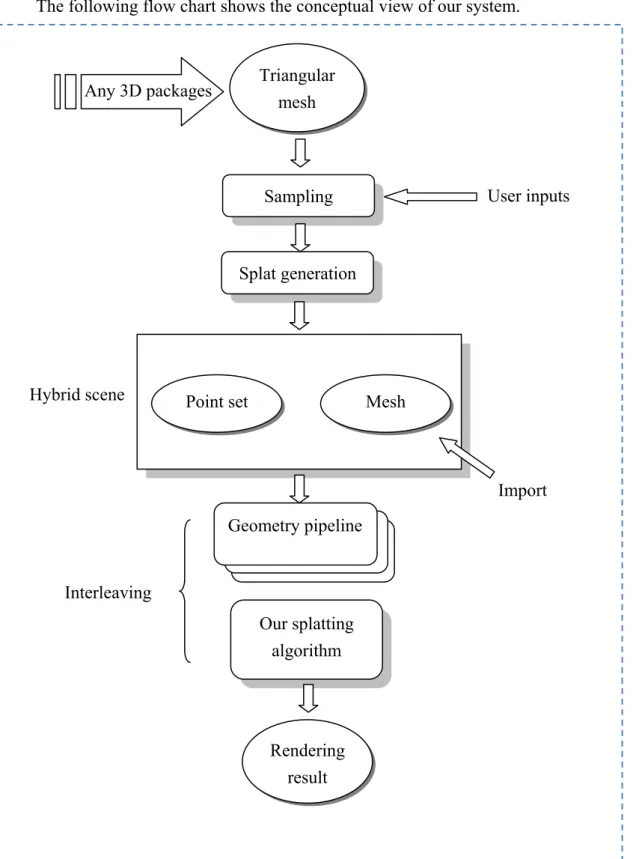
The following flow chart shows the conceptual view of our system. Triangular

mesh Sampling

Point set Mesh

User inputs Our splatting algorithm Sampling  Sampling  Geometry pipeline Rendering result Splat generation Any 3D packages Hybrid scene Interleaving Import

Taking a triangular mesh constructed by any available 3D packages as inputs, our system first samples the mesh to generate an initial point set. At this stage, the point set only contains the most basic data directly capture or derived from the input mesh, e.g. position, normal and material information. For rendering purpose, we then pass the set to the splat generation stage. Here our system assigns all the necessary information to the point set for splatting, e.g. tangent coordinates and dimensions, and disposes unnecessary points. For a scene consists of both point-set models and triangular meshes, we call it a “hybrid scene”. We implement our splatting algorithm with the principle that it may be easily integrated into existing rendering algorithm for triangular meshes, which we use the term “geometry pipeline” in figure.1 since the processing of the two is quite different. The final result may be obtained by rendering objects with arbitrary order in our implementation.

1.3 Thesis Organization

In the following sections, we first introduce related previous works of techniques related to point-set models in chapter 2. In chapters 3 and 4, we describe the sampling and the splat generation algorithm that we use to produce point-set model. Our rendering algorithm will then be described in chapter 5 in detail. Finally, we show our results, benchmark, and discussions in chapters 6 and 7, respectively.

Chapter 2: Related Works

Using points as primitives was first proposed by Levoy and Whitted [15]. Because of the development of technology of range scanners and the conceptual simplicity of a point, many works were devoted to this field since then. However, efficient rendering of point-set models was not possible until the work by Grossman J. P. and Dally W. J. [9]. They developed an image-space surface reconstruction algorithm and made a great step forward in both the rendering performance and quality. Later, QSplat [23] introduced splat with flat-shading quality and multi-resolution data structure to deal with massive point sets.

Alexa M. et. al. [1] introduced the concept of MLS (moving-least-square) fitting with respect to a plane. It soon became the main trend of the surface definition of point set because of its great approximation of the surface and indefinitely differentiability [13], [14]. Recently, Guennebaud G. and Gross M. [11] suggested to define the surface with MLS fitting with respect to algebraic surface to gain more accuracy.

Zwicker M. et. al. [29] presented a pure software implementation of EWA(elliptical-weighted-average) splatting and achieved superior rendering quality and handled transparency correctly. Many works were then devoted to develop an efficient way to implement EWA splatting on graphics hardware [3], [4, [5, [22]. Recently, Weyrich T. et. al. [27] further presented a prototype of graphics adapter for EWA splatting.

The LOD of point-set model was also investigated for efficiency. QSplat [23] organized points as bounding-sphere hierarchy and gained a great performance and memory efficiency via densely encoding node information. For solving depth order and LOD, Zwicker M. et. al. [23] and Pfister H. et. al [21] first introduced layered-depth cube (LDC), which is basically an improved version of layered-depth map [24]. Dachsbacher C. et. al. [8] developed a LOD structure which may process and select level entirely on graphics adapter.

Since point set may represent complex geometry efficiently while triangle may be a better choice for broad flat region and sharp features, hybrid representation of were investigated [6], [7], [8], [10]. They rendered and blended the surface color of triangles and point-set models when it was a faster option. Müller M. et. al. [17] expanded the definition of a splat with clipping lines to render sharp features solely with splatting algorithm.

The unstructured property of point-set models also drew interests in the field of modeling and physical-based animation. PointShop3D [31] first proposed a modeling package of point-set models. Following, Pauly M. et. al. [20] developed more robust and complete solution. Müller M. et. al. [17], [18] pioneered the field of meshless animation.

Chapter 3: Mesh Sampling

Our sampling algorithm is basically an improved version of the stratified sampling proposed in [19]. It first converts meshes to voxel approximation by constructing an octree, and then generates a sample point per voxel with respect of a radial function. The reason of [19] is to overcome the drawback that area-based uniform sampling algorithm often failed to spread enough sample point over complex region of the mesh [26]. With stratified sampling, we may ensure better spatial uniformity of sampling points over the whole mesh.

Nevertheless, the original algorithm in [19] has two insufficiencies. First, it lacks of importance criteria. Second, it doesn’t provide user with the ability to define one’s desired sample count with respect to a voxel approximation level. We improve these via introducing priority during sampling and allow user to define the number of sample points in a level.

Figure 2 is an overview of the whole sampling process. By substituting the priority function and the distribution function, our system may change the perspective on importance region totally, while maintaining the spatial uniformity. Thus it can be viewed as a framework, not just an algorithm.

In the following sections, we use the term “leaf cell” and voxel alternatively, since they are the same in this context. In section 3.1, we first describe how we do the voxelization. We then present our sampling algorithm and how we define attributes of each sample point in section 3.2. Finally, we show results in section 3.3.

Mesh Voxel approximation Priority function Sampling Voxels Voxel heap

The voxel with the highest priority value Update

Insert

Minimize the priority value of the voxel Reach the user-specified

sample count

Sample points Figure 2 Overview of the sampling process

3.1: Voxel Approximation

We compute the voxel approximation of the input triangular mesh via a top-down octree construction algorithm like [19]. First, the axis-aligned bounding box is computed and is taken as the root cell. Next, we recursively divide the cell with respect to the longest dimension, and store triangles which intersect with the cell. To detect whether a triangle and a cell intersect, we found that the fast triangle-box overlap testing procedure presented by T. Akenine-Mäoller [2] is very efficient and is easily integrated. The recursion stops whether the user-defined depth reached or no triangle is recorded in the cell. After the whole process terminates, each leaf cell contains the following information:

Position: The center position of a voxel.

Dimensions: Since our cell is axis-aligned, these are dimensions in x, y, z axis. Triangles: Triangles which intersects with the voxel.

Priority value: As its name implies, it defines the importance estimation of a voxel. It

is computed by the priority function pre-defined by the system. Our system then spreads the sample points according to this value. We use the number of triangles as the default priority function.

3.2: Priority-Based Stratified Sampling

Distribute sample points

Our system allows user to input the number of sample points. Because we sample the mesh according to the voxel approximation, there are two scenarios: the user defined amount is equal to or greater than the number of voxels, or it is less than the number of voxels.

Apparently, the second scenario is not recommended since it lefts some regions un-sampled. We sort the voxels according to its priority value, and then assign sample points in descending order.

Back to the first scenario, we first compute the priority value of each voxel via the priority function. Then, we reorganize these voxels to a heap. With the help of heap, we may easily get the voxel with the highest priority value. Since we hope each sample point contains as much information as possible, our strategy is to minimize the priority value of a voxel after sampling. We then update the priority value and insert the sampled voxel back to the heap. In this way, we may ensure the voxel with higher priority value may produce more sample points than lower one. After the sample count reaches the user-specified value, the process terminates.

Assign attributes

For each point generated in the distribution phase, we first project it onto the surface defined by the triangles recorded in the voxel. The projected point will lie on one of the triangle. In some rare case, it will lie on edges or vertices. We then choose the first encountered one. Next, we compute the barycentric coordinates of the projected point. Finally, we interpolate the attributes with the barycentric coordinates and get the final sample point. A sample point may contain arbitrary information defined or derived on the mesh. In our implementation, each sample point contains position, normal, texture coordinates, and material information.

3.3 Examples of Sampling

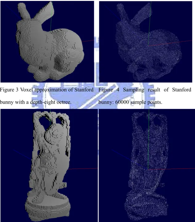
Here we show some results of our sampling algorithm. Figure 3 and Figure 5 are samples of the voxel approximation. Figure 4 and Figure 6 are sampling results from them.

Figure 3 Voxel approximation of Stanford bunny with a depth-eight octree.

Figure 4 Sampling result of Stanford bunny: 60000 sample points.

Figure 5 Voxel approximation of happy budda with a depth-eight octree.

Figure 6 Sampling result of happy budda: 35000 sample points.

Chapter 4: Splat Generation

After sampling, we further process and convert the set of sample points to a set of splats using a simplified version of the optimized sub-sampling algorithm by J. Wu and L. Kobbelt [28]. It generates optimized hole-free ellipse splat set which approximates the input point set within a prescribed error tolerance ε. While the error tolerance is maintained, our system generates circular splats, apply more conservative coverage estimation.

There is no doubt that our simplification will lost several good features. Using elliptical splat provides anisotropic filtering, and is proven that can obtains the same visual quality with less number of splats then circular splats would need [3], [28]. With the global relaxation, the regularity is improved, and geometric features can be captured with possibly less splats. However, the main goal of our system is not to generate optimized splat representation. In all of our experiments, this simplified algorithm does well.

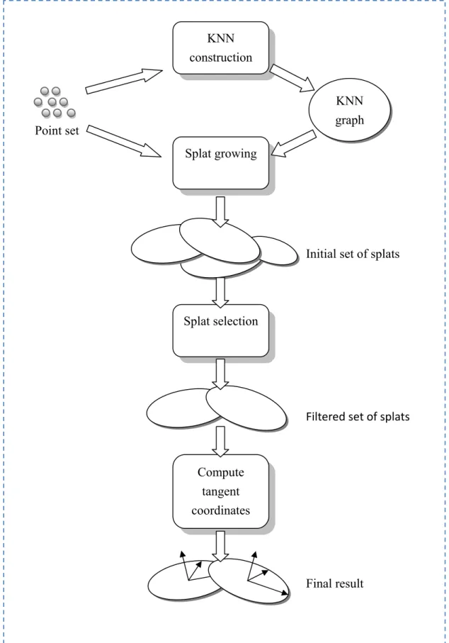
Figure 7 is an overview of the whole splat generation process. In the following sections, we discuss each stage thoroughly. Be aware of the difference between “point” and “splat”. A point is the sample point generated from the sampling stage and is a zero-dimensional object, while a splat is grew from a point, a circular disk with its own tangent coordinates.

KNN construction Point set Splat growing KNN graph

Initial set of splats Splat selection Compute tangent coordinates Filtered set of splats  Final result

4.1: KNN Graph Construction

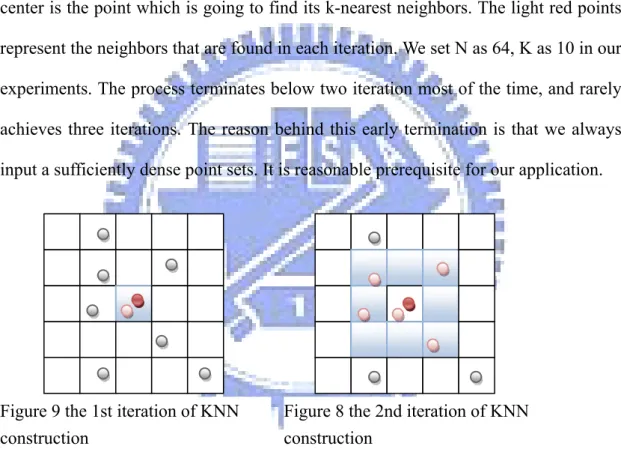
The first step of our algorithm is to construct the k-nearest-neighbor graph of the input point set. We divide the space into an N×N×N grid, iterate through the point set, and register the point to the grid cell which contains it. With this uniform grid, we may easily find k-nearest neighbors for each point by traversing the neighboring grids. A 2D conceptual view is presented in Figure 8 and Figure 9. The dark red point at center is the point which is going to find its k-nearest neighbors. The light red points represent the neighbors that are found in each iteration. We set N as 64, K as 10 in our experiments. The process terminates below two iteration most of the time, and rarely achieves three iterations. The reason behind this early termination is that we always input a sufficiently dense point sets. It is reasonable prerequisite for our application.

Undoubtedly, there are many works done in the construction of KNN graph which definitely outperform than ours [25]. However, the whole splat generation process is a preprocessing stage. It seems to be unpractical comparing the performance gained by implement those cleverer algorithms and the work time it may need for us. Further, in our experiments, this simple algorithm does provide acceptable performance.

Figure 9 the 1st iteration of KNN construction

Figure 8 the 2nd iteration of KNN construction

4.2: Splat Growing

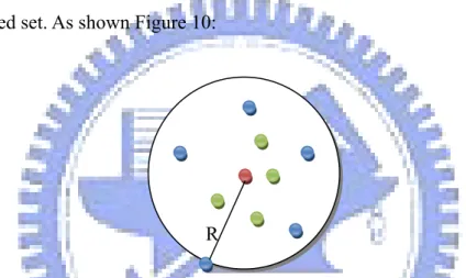
The way we growing splats from the input point set is basically the same as [28]. For each point, we generate a corresponding splat and take the position of the point as its center. Then, we traverse the KNN graph in a breadth-first manner. For each traversed point, we check whether its deviation from the tangent plane exceeds the error tolerance. If the error tolerance is not exceeded, we record the outer-most encountered points in the confront set, and the points inside the splat are recorded in the conquered set. As shown Figure 10:

The difference between a confront point and a conquered point is that, a confront point has not yet been expanded by the breadth-first traversing, while the conquered point has been expanded. I.e. there exists at least one point farther from the center than the conquered point. Thus it is definitely inside the splat. The process terminates if the error tolerance is exceeded. Please consult [28] if further details are needed.

R

Figure 10 A concept view of the relation of different point set. The red point is the center of the splat. Blue points represent the confront set. Green points are the conquered set. R is the radius of the splat.

4.3: Splat Selection

After growing splats, we select a subset of splats which cover the whole surface defined by the input data. As in [28], we define a surface area element with each sample point, say p,

       1

where d is the distance to the k-th neighbor. We may then define the surface area contribution, say Q, of a splat by summing up the surface area element of a sample point:

      2

A greedy selection algorithm based on the surface area contribution is then applied. In each step we select the splat with the highest surface area contribution, and traverse through the other splats to reduce the surface area element associated with the selected splat. The process stops if all the surface area contribution becomes zero, which indicates that the whole surface area is covered. With this terminating condition, we may ensure that all the splats represent delicate details will be selected. Since such a splat often has a conquered set containing itself solely, the only way to reduce their area contribution to zero is to select them.

Hole-free approximation

Indicated by [28], to select a hole-free set of splats is actually a NP-hard dominating set problem. The approximation algorithm they proposed is to project the conquered set, Q, onto the tangent plane of the splat, construct a 2D convex hull, C, and use Q – C as a new coverage relation. Our approximation is simpler and heuristic. We simply adjust the radius of a splat with a constant ratio R, and apply this new

radius to define the conquered set. Though not as general as the original work, setting R as 0.5~0.7 does well in all our experiment.

4.4: Define Tangent Coordinates

The most general way to define tangent coordinates is to apply mean-least-squares fitting to find normal, and then compute maximal and minimal principal curvature as tangent axis [3]. This method may apply to any kind of point set, especially when the source is a 3D scanner and the only available information within a point is position [1]. Our point set is sampled from a mesh. The attribute assigning stage in sampling process already gives us ideal normal. Furthermore, we only grow circular splats here, and thus any two vectors that are orthonormal to each other and the normal can form a reasonable tangent coordinates. Finally, in our implementation, the tangent coordinates are formed by the normal, the projection of x-axis onto the tangent plane, and the projection of y-axis onto the tangent plane.

4.5 Examples of Splat Generation

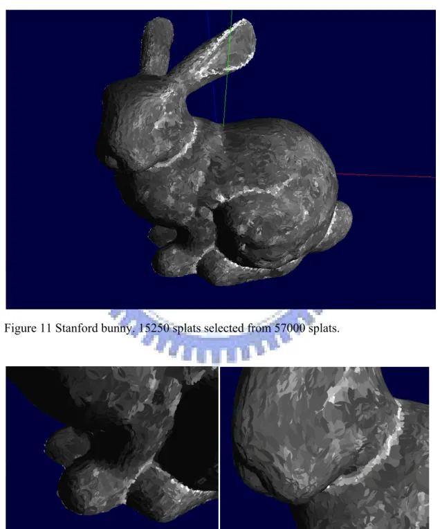
Here we show some results of our splat generation process. Figure 11 is a Stanford bunny formed by 15250 splats selected from the original 57000 splats. Notice that the hole-free property is well-preserved by our simplified algorithm.

Figure 11 Stanford bunny. 15250 splats selected from 57000 splats.

In the following figure, we shrink the splats to show a clearer view of splats. In figure 13, we may see that those small splats represent detail parts (tiny white splats) of the mesh are preserved by the selection stage. Figure 14, we show the affection by omitting the global relaxation.

Figure 13 A clearer view of splats. Notice that the details (small splats) are preserved.

Chapter 5: Rendering

Rendering a point-set model can be viewed in two different perspectives. In the computational-geometry point of view, the surface defined by projecting the point set to the moving-least-square surface defined by the point set itself will be an indefinitely differentiable surface [13], [14]. Thus, any implicit surface rendering techniques can be applied, e.g. ray-casting algorithm. However, it seems to be unpractical when high performance of rendering is significant because of the cost of computing implicit surface. In the view of signal processing, if we take the surface attributes of the input mesh as a spatial signal, then rendering a point-set model becomes a spatial signal reconstruction problem. We now further discuss this perspective.

EWA splatting [29] is a technique with the highest rendering quality so far in our knowledge. It is originated from the work of Heckbert [12], which applying elliptical-weighted-average filter for texture filtering. It assigns an elliptical Gaussian reconstruction filter to each splat, and convolves it with a band-limited filter, which is called the object space EWA filter. If the band-limited filter is again a Gaussian, then the projection on the image plane is still a Gaussian, which is referred to as the image space EWA filter. Projecting and accumulating these reconstruction kernels on the image plane produce the final image output. The whole process may be considered as signal reconstruction in object space or image space. For a complete derivation, we recommend the article by Zwicker M. et. al. [30].

grab great interests on implementing hardware-accelerated EWA splatting. Many great works were done in facilitating of pixel shader to rasterize EWA filter on screen space [3], [4], [5]. The point sprite like OpenGL point [3] or NV_sprite [5] provide an ideal way to generate enough fragments to rasterize EWA filter. To rasterize the filter, the first step is to discard unnecessary fragment via the inside test,

u v ·   ·   1        3

where u and v are tangent coordinates, c is the center, and q is the input point. With the position and the normal of the splat, the algorithm may then rasterize the shape of the filter correctly. However, since a point sprite is actually a billboard aligned with image plane, depth correction is necessary against incorrect depth occlusion artifacts. Botsch M. and Kobbelt L. [4] first presented an implementation with Gouroud shading quality. Phong splatting [3] soon achieved phong shading quality by associating a linear normal field with each splat. Botsch M. et. al. [5] introduced the idea of deferred shading in EWA splatting and improved the performance further.

Ren L. et. al. [22] proposed an object-space approach. The idea was to render EWA filter with a quad textured with a unit-Gaussian map. In this way, the perspective transform is automatically accurate and is computed by hardware. The rasterization of EWA filter also did not need any special care since it was done by rasterizing the textured quad. Further, it didn’t need depth correction. However, the performance was slower than most of the screen space approach because of the hardware constraints.

No matter object-space or screen-space approach is used, a common issue occurs: how to blend splats contribution? Since each EWA filter is truncated to a finite

support, it is reasonable to blend only the splats which deviate in z direction of eye coordinates under some threshold values. I.e. the z-test is not simply 0 or 1 anymore; it contains a small tolerance range and thus the name “fuzzy-z test”. Unfortunately, there is no way to implement this fuzzy-z test directly under current graphics hardware since the depth-stencil test stage is not yet programmable. One way to solve this problem is to apply other visibility technique. Layered-depth cube is a common choice and has been widely investigated [4], [21]. The other trend is to introduce a visibility pass to the rendering process [3], [4], [5]. It only generates depth map. One simply “moves” it along the viewing direction the amount of tolerance range [22], and then the traditional depth-stencil test will behave as fuzzy-z test.

Nevertheless, with this fuzzy-z test, rendering a scene with triangular meshes and point-set models become a tricky task. The point-set model will appear to merge with the triangular mesh when their depth value is within the tolerance range. A naïve approach may be render the point-set model in a different render target, and then merge it back according to the depth buffer. However, depth occlusion artifacts occur on the intersection region with this approach. Figure 15 shows a point-set Stanford bunny intersects to a triangular-mesh Utah teapot. These artifacts occur because the depth value of the point-set model is computed from the tangent plane of each splat lied on, not from the surface itself.

  Figure 15 Stanford bunny intersects to Utah teapot

Thanks for the new shader 4.0 specifications, we may efficiently construct object-space EWA filter with geometry shader now. We further combine the deferred shading proposed in [5], and implement it with the new feature in shader 4.0 which allows us to render to multiple render targets concurrently in primitive level. Our rendering algorithm is a multiple-pass algorithm like [5]. The visibility pass generates depth map. The attribute pass render the color, normal, and any desired attributes to different render targets. Finally, the shading pass reads in these attribute maps and renders the final result. In this thesis, we further generalize the attribute pass to deal with depth occlusion artifacts.

5.1: Pass 1: Visibility Pass

Figure 16 shows the rendering pipeline of the visibility pass.

The main goal of this pass is to generate the depth map for the following fuzzy-z test. We first pack the whole splat set into a vertex buffer, and set the primitive type as point list. The vertex shader in this pass transforms the position and tangent

Vertex shader Geometry shader

Input assembly

Pixel shader Splat set

Packing as vertex buffer

Generate a

corresponding quad

Output merger Set render target as

NULL

Depth map Figure 16 Rendering pass 1: visibility pass

coordinates to world space, and then passes the data to the geometry shader. The geometry shader then generates a quad corresponding to each splat, and transforms them to the projection space, as shown in Figure 17.

Before any draw call is made, we set the render target as NULL. Thus we get a depth map in this pass without affecting any previous rendering result in the framebuffer.

u v

urad vrad

Figure 17 The quad generated by geometry shader. The red point is the center of the splat, and blue points are points generated by geometry shader.

5.2 Rendering Pass 2: Attribute Pass 

Vertex shader Geometry shader

Input assembly

Gaussian map

Pixel shader Depth _map

Multiple render targets

Output merger Set depth buffer as _NULL

    Attribute maps Generate corresponding quad in number of attribute maps

In this pass, the vertex shader transforms the position, normal and tangent coordinates to the world space. The geometry shader again expands the point into a quad, then assigns desired attributes in the color channel, and sends them to the correct render target via SV_RenderTargetArrayIndex semantic. The depth buffer is set NULL at the beginning and is fed as a shader resource. In the pixel shader, we first do the inside test as equation (3) to discard unnecessary pixels. Although it is an optional step for object-space approach, we found that discard these pixels may increase some performance. Next, it read depth buffer to do fuzzy-z test. Given that a value, zb, read from the z buffer. Since it is a value defined in the normalized device

space, we need to transform it back to the projection space, z   FN

F z F N        4

where F stands for the far clipping plane, N stands for the near clipping plane. We then use this value to perform the fuzzy-z test.

After processing two tests described above, we then render the quad with the prescribed unit Gaussian map as alpha texture. By using the floating-point precision render target and enabling alpha blending, surface attributes are accumulated and blended correctly in each render target:

w h ,   h           5

where x is the position, xi is the splat center, h is the reconstruction kernel and thus

the Gaussian in this thesis. C stands for the (R, G, B) channel, and alpha stands for the alpha channel. We then do a per-pixel normalization by dividing the color value with alpha value:

w h

In the original work of Bostch M. and Kobbelt L. [5], they generated a color map and a normal map in this pass. The color map was basically the blending result of the material color and the diffuse texture. The normal map was the blending result of normal vectors as the name described. Here we further generalize the application of the attribute pass to deal with texturing and eliminate depth occlusion artifacts.

Texturing and depth correction: TexZ map

As mentioned in the first paragraph, the EWA splatting is actually a spatial signal reconstruction process, and the spatial signal can be any surface attributes. Since our point-set model is obtained from sampling a triangular mesh, we may reconstruct the parameterization of the surface by sending the texture coordinates to the attribute pass. Further, we may also consider the depth value of each sample point in the projection space as a surface attribute and reconstruct the depth value of the surface. Our current implementation only considers 2D texture-space parameterization; thus we may pack the 2D parameterization and the projection-space depth value, and render it into one render target. Since it consists of 2D parameterizations for texturing and depth, we name it TexZ map.

5.3 Pass 3: Shading Pass 

Figure 19 shows the rendering pipeline of the shading pass.

In this pass, we take color map, normal map, depth correction map, and any other possible attribute maps generated in the attribute pass to compute the final result. First, we set geometry shader and the input layout as NULL. In vertex shader, we use the system value: SV_Vertex_ID to generate a viewport-sized quad.

Vertex shader Geometry shader Input assembly Pixel shader Normal map Generate a viewport-sized quad Output merger

Set the depth buffer again Set input layout as NULL Final output     Attribute maps Depth map TexZ map

For each pixel, we first load the value from TexZ map by screen coordinates and discard it if its alpha value is zero. Of course, this check can be done with any attribute map. Next, for each pixel passing the alpha test, we compute its color value. It is basically color_value + lighting_component, where color_value is fetched from the diffuse map with texture coordinates in TexZ map, and the lighting_component is computed via the normal fetched from the normal map. All the value fetching mentioned above uses the intrinsic function Load(). Since they are all viewport-sized, we don’t need any filtering. After fetch the value, we do per-pixel normalization as in [5].

Notice that we turn on the output channel to the depth buffer in our pixel shader. Since the z value stores in the TexZ map is in the projection space, we need to transform it to the normalized device space before output:

z F F N 1

N

z           7

Thus any following rendering techniques will then have proper depth information of our point-set model.

Chapter 6:   

Results and Discussion 

6.1 Rendering Results 

  Figure 20 Happy budda rendering with 170000 splats. From left to right: shading result, normal map, and depth correction map. With smoothly blended normal, we may easily achieve Phong shading quality.

  Figure 21 A textured cloth.

  Figure 22 A textured long dress. Note that the spatial aliasing around the edge are caused by the nature of splats.

(1)

(2)  Figure 24 Result of the depth correction. (1): Without depth correction. (2): With depth correction.

  Figure 25 A point-set clothes on a triangular-mesh man. With our depth correction technique, we may try to make a close contact between point-set models and triangular meshes without depth occlusion artifacts.

  Figure 26 Bunnies in grass. The scene consists of 231986 splats and 50553 triangles. Bunnies and rocks are point-set models while grass and carrot are triangular meshes. The scene is rendered at 55 FPS on 8800GTX

6.2 Performance and Discussion 

In this section, we discuss performance issues in detail. The performance was measured on a machine with GeForce 8800GTX card, the version of the driver was 172.20, and the screen resolution was 1024×768. The algorithm was implemented with DirectX SDK ver. March 2008. Our implementation achieves 16M splats/sec in average.

It turns out that graphics adapter and the bandwidth between CPU & GPU dominates the performance, since CPU does nothing but sends data to graphics adapter in our system. Please note that we didn’t apply any LOD technique in our experiment and thus the performance “seems to be” far slower than those pioneer works [3], [4], [5], [29].

Backface culling

After a point is expanded to a quad in the geometry shader, the default backface culling will be performed in the output merger stage. Nevertheless, we may do backface culling in the geometry shader in advance to prevent generating redundant quads. We gain a performance raise of 1M splats / sec in average by doing so.

MRT controlled at primitive level

The shader model 4.0 introduces a new feature that controlling MRT at primitive level. One may easily generate primitives in a geometry shader and rasterizes them to different render targets with system-value semantic, SV_RenderTargetArrayIndex.

Chapter 7:

Conclusions & Future Works

In this thesis, we try to investigate some of the basic techniques of hybrid scene representation. We name two fundamental issues: data source of point-set model and an easily-integrated rendering module. We first present a novel priority-based stratified sampling to convert a triangular mesh to a point set, and then grew a corresponding splat representation from it with a simplified version of [28]. Our priority-based sampling can be viewed as more a framework than simply an algorithm.

The idea of generalized attribute pass may be worthy of further investigation. In our experiment, reconstructing 2D parameterization in this way turns out to be very sensitive to the quality of sampling. A not-good-enough sampling may cause overly blurred results using textured splats like [22], but cause an obvious distortion in our system. Currently, our priority-based sampling applies the number of triangles as priority value. It cannot correctly capture the high-spatial-frequency region with a small number of triangles. Figure 25 shows an example. While the body of the zebra is textured correctly, the sharp region around the head shows serious distortion. Applying a priority function based on the gradient of distance field might produce better results. A better splat generation will also improves the overall quality.

Figure 27 A failure case of texturing. Notice the distortion around the head. These artifacts are caused by bad sampling quality around the high frequency region.

As shown in Figures 21, 22 and 25, our system doesn’t handle sharp edges properly. Associating clipping lines with splats might be a solution. The way to defining clipping line automatically in the splat generation stage may be worth to investigate.

Our current implementation rendered with a raw data set. Integrating a LOD technique will undoubtedly boost the performance. To not conflict with our basic principle: easily-integrated with exist triangular mesh rendering modules; we anticipate that a LOD technique suits for GPU, like sequential point trees [8], will be an ideal choice.

References

1. Alexa M., Behr J., Cohen-Or D., Fleishman S., Levin D., and Silva C. T., Point Set Surfaces. IEEE Visualization, 2001.

2. Akenine-Mäoller T., Fast Triangle-Box Overlap Testing.

3. Botsch M., Spernat M., and Kobbelt L., Phong Splatting. Eurographics Symposium on Point-Based Graphics, 2004.

4. Botsch M., and Kobbelt L., High-Quality Point-Based Rendering on Modern GPUs. Proceedings of the 11th Pacific Conference on Computer Graphics and Applications, 2003.

5. Botsch M., Hornung A., Zwicker M., and Kobbelt L., High-Quality Surface Splatting on Today’s GPUs. Eurographics Symposium on Point-Based Graphics, 2005.

6. Chen B., and Nguyen M. X., POP: A Hybrid Point and Polygon Rendering System for Large Data, IEEE Visualization, 2001.

7. Coconu L., and Hege H. C., Hardware-Accelerated Point-Based Rendering of Complex Scenes. Thirteenth Eurographics Workshop on Rendering, 2002. 8. Dachsbacher C., Vogelgsang C., and Stamminger M., Sequential Point Trees,

SIGGRAPH 2003.

9. Grossman J. P. and Dally W. J., Point Sample Rendering, Proceedings of Eurographics Rendering Workshop ’98 page. 181-192, 1998.

10. Guennebaud G., Barthe L., and Paulin M., Splat/Mesh Blending, Perspective Rasterization and Transparency for Point-Based Rendering, Eurographics Symposium on Point-Based Graphics, 2006.

2007.

12. Heckbert P., Fundamentals of Texture Mapping and Image Warping. Master’s Thesis, University of California at Berkeley, Department of Electrical

Engineering and Computer Science. 1989.

13. Levin D., The Approximation Power of Moving Least-Squares. Mathematics of Computation, Vol. 67, No. 224, October 1998, pages 1517-1531.

14. Levin D., Mesh-independent Surface Interpolation. Geometric Modeling for Scientific Visualization. Springer-Verlag, 2003.

15. Levoy M. and Whitted T., The Use of Points as Display Primitives. Technical Report TR 85-022, the University of North Carolina at Chapel Hill, Department of Computer Science, 1985.

16. Marroquim R., Kraus M., and Cavalcanti P. R., Efficient Point-Based Rendering Using Image Reconstruction. Eurographics Symposium on Point-Based Graphics, 2007.

17. Müller M., Heidelberger B., Teschner M., and Gross M., Meshless Deformations Based on Shape Matching. ACM SIGGRAPH, 2005.

18. Müller M., Keiser R., Nealen A., Pauly M., Gross M., and Alexa M., Point Based Animation of Elastic, Plastic, and Melting Objects. Eurographics/ACM

SIGGRAPH Symposium on Computer Animation, 2004.

19. Nehab D., and Shilane P., Stratified Point Sampling of 3D Models, Eurographics Symposium on Point-Based Graphics, 2004.

20. Pauly M., Keiser R., Kobbelt L. P., and Gross M., Shape Modeling with Point-Sampled Geometry. ACM SIGGRAPH, 2003.

21. Pfister H., Zwicker M., Baar J., and Gross M., Surfels: Surface Elements as Rendering Primitives, ACM SIGGRAPH, 2000.

22. Ren L., Pfister H., and Zwicker M., Object Space EWA Surface Splatting: A Hardware Accelerated Approach to High Quality Point Rendering, Eurographics 2002.

23. Rusinkiewicz S., and Levoy M., QSplat: A Multiresolution Point Rendering System for Large Meshes. SIGGRAPH, 2000.

24. Shade J., Gortler S. J., He L., and Szeliski R., Layered Depth Images. In

Computer Graphics, SIGGRAPH 98 Proceedings, pages 231-242. Orlando, FL, July 1998.

25. Sankaranarayanan J., Samet H., and Varshney A., A Fast K-Neighborhood Algorithm for Large Point-Clouds. Eurographics Symposium on Point-Based Graphics, 2006.

26. Turk G., Generating Textures on Arbitrary Surfaces Using Reaction-Diffusion, Computer Graphics, Vol. 25, No. 4, July 1991.

27. Weyrich T., Heinzle S., Aila T., Fasnacht D. B., Oetiker S., and Botsch M., A Hardware Architecture for Surface Splatting. ACM SIGGRAPH, 2007. 28. Wu J., and Kobbelt L., Optimized Sub-Sampling of Point Sets for Surface

Splatting, In Proceedings of Eurographics 04, pages 643-652.

29. Zwicker M., Pfister H., Baar J., and Gross M., Surface Splatting, ACM SIGGRAPH, 2001.

30. Zwicker M., Pfister H., Baar J., and Gross M., EWA Splatting. IEEE Transactions on Visualization and Computer Graphics, Vol. 8, No. 3, July-September 2002.

31. Zwicker M., Pauly M., Knull O., and Gross M., Pointshop 3D: An Interactive System for Point-Based Surface Editing. In Proceedings of SIGGRAPH 2002.