Improvement and Evaluation of Visual Saliency
based on Information Theory
Anh Cat Le Ngo, Li-Minn Ang, Kah Phooi Seng
School of Engineering
The University of Nottingham, Malaysia Campus Jalan Broga, 43500 Semenyih, Malaysia Email: keyx9lna,kezklma,[email protected]
Telephone: +60 3 8924 8350 / 8000 Fax: +60 3 8924 8017
Guoping Qiu
School of Computer Science The University of Nottingham, UK Campus
C34, CS Building, Nottingham, UK Email: [email protected] Telephone: +44 115 8466507
Fax: +44 115 9514254
Abstract—Visual saliency is a well-known image processing technique based on theory about visual attention of human beings. Several proposed computing approaches based on findings in psychological and neurological researches about the part of human brain area in charge of visual attention. Contrast to those methods, in this paper the information theory is recommended as backbone for a new approach of building visual attention computer model, assumed that the uniqueness of a pixel or a group of pixels correlates with saliency. The information saliency is identified in both spatial domain and temporal domain, and eventually those two pieces of information is combined in a mathematical integrated framework naturally. Experiments of the model on intensity, contrast, and especially full motion video show that its performance is comparable to other state-of-art saliency approaches. Though there are still minor flaws in the information based saliency, it is a potential alternative approach for visual attention in video-based applications.
Index Terms—spatial-temporal saliency, evaluation, saliency, etc
I. INTRODUCTION
Visual attention derives important information for visual content analysis in widespread fields such as content-based searching algorithm for multimedia, image and video com-pression. It is especially useful in real-time scenes content-based analysis, the basic block in building highly efficient machine vision systems. Up until very recently, most research in computer model for visual attention has focused primarily on still images [1], [2], [3], [4] and low-level image features such as color, intensity, and contrast are heuristically used to detect visual attentive regions. With main concentration on still images and their spatial characteristics, the motion and other temporal features ,supposed to attract most human attention, were left undiscovered.
Recently, some researchers [5], [6], [7] have made initial steps in investigating the importance of temporal-domain fea-tures. A common approach is forcefully deploying methods of spatial saliency on motion features. After independently calculating spatial and temporal saliency scores, they are fused together in some arbitrary manners. An assumption of equal contribution between spatial and temporal domain is usually made, hence the integrated spatial temporal saliency is an average value. Those ad-hoc approaches have made
two unreliable assumptions: equal contributing weights of spatial and temporal features, and motion feature extraction. How the motion estimation should be extracted is still in debate. In addition, more researches need to be done to prove direct relations between motion estimation and human visual attention. Even assuming these previous two queries were satisfactorily answered, there would be still other obstacle how spatial and temporal factors affect on human vision. Thence it is unclear how to fuse those features together in computational models.
While most of the saliency methods use visual contrast on several features such as intensity, colour, and motion to calculate saliency values, Shannon’s self-information was proposed as an appropriate measure for the perceptual saliency in still images by Topper [8]. Though the idea was originally advised by Topper, it was only realized and tested on still images by Bruce [2]. Through Bruce’s research, the correlation between local statistics and saliency objects was assured on, again, still images only. Until the research done by Qiu [9], similar relation was extensively analysed in video context; in addition, a simplified computational model has been suggested to relate local statistical information to saliency scores in both spatial and temporal domains.
In this paper, similar information theoretical model is exam-ined but different computational model is proposed to calculate saliency from self-information. Moreover, in section III the mathematical models are tested on several defined images so as to find out its pros and cons. Section IV showing simulation results on sequences of continuous images prove the proposed visual saliency model is practical and well-performed for video context.
II. INFORMATIONTHEORYAPPROACH
The information theory approach adopts ideas of Shan-non theory about self-information into saliency calculation instead of visual contrast approach mentioned in other popular saliency methods. In the Shannon’s information theory, unique and highly rare events contain large amount of information, and this ”uniqueness” or ”informationess” can be deferred into images, containing 2-D data as well. The theory is usually
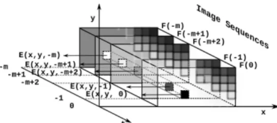
y -1 0 -m+2 -m+1 -m t F(0) Im ag e Se qu en ce s F(-m) F(-m+1) F(-m+2) F(-1) E(x,y, 0) E(x,y,-m) E(x,y,-m+1) E(x,y,-m+2) E(x,y,-1)
Fig. 1: An illustration of spatial and temporal events. In the space domain , the frame Ft at t = 0 is divided in n
blocks (patches) E(x, y, 0), Es1(x1, y1,0), ...E(xn, yn,0). In
the time domain, each block ,E(x, y, 0), is seen as an event and the evolution of this event over time is recorded in a set
Vx,y = {E(x, y, 0), E(x, y, −1), ..., E(x, y, −m + 2),
E(x, y, −m + 1), E(x, y, −m)}.
described under following mathematical formula.
Iinf ormation= − log(P (E(x, y, t))) (1)
where Iinf ormation is the amount of self-information or
saliency score contained in event E(x, y, t). Direct ties between information theory and saliency has been clarified clearly, so now the computational task becomes of finding the probability P(E(x, y, t)). Before presenting computational methods, there is a need of clearly defining events and factors affecting their ”informationess” and ”uniqueness”. In videos, an event E(x, y, t) may be a pixel of whose saliency can be theoretically found, depending where that pixel is located and at which frame it happens. However, the event E(x, y, t) may also be a group of pixels and its uniqueness also depends on how often the same blocks repeat in its spatial and temporal domain. As the event E(x, y, t) is seen as a block of pixels, it reduces computational cost and makes information method more practical. For a given
E(x, y, t), its spatial domain is defined as Ft(x, y) =
Es0(x0, y0, t), Es1(x1, y1, t), Es2(x2, y2, t), ..., Esn(xn, yn, t)
and its temporal domain is a set of Vx,y(t) =
Et0(x, y, t0), Et1(x, y, t1), Et2(x, y, t2), ..., Etm(x, y, tm).
The informationess of spatial-temporal event E(x, y, t) depends its spatial and temporal contexts. If the event, block of pixels E(x, y, t), rarely occurs in the same frame or spatial context, obviously the block should have higher salient values. Similarly, if the patch E(x, y, t) is unlikely to repeat itself during its evolution over time, its ”uniqueness” or ”informationess” is high, so is its temporal saliency value. Obviously, the spatial and temporal environments jointly influence informationess and uniqueness of an event. Therefore, the computer task now is to identify its chance of occurrence in spatial and temporal contexts.
A. Information Theory Model
Assumed that there is direct relation between uniqueness of an image and its saliency, the spatial-temporal saliency
ST S(x, y, t) can be modelled by the amount of information
from events E(x, y, t). Moreover, the saliency values are
undoubtedly influenced by its surrounding time and space en-vironment and so is the information in E(x, y, t) according to Shannon’s information theory ,given its spatial context Ftand
temporal context Vx,y. Later, variables x, y, t will be truncated
in some the equations, for examples, E(x, y, t), Ft(x, y) and
Vx,y(t) will become E, Ft and Vx,y only.
ST S(x, y, t) = −log(P (E|Vx,y∩ Ft) (2)
The equation 2 represents the information model which ele-gantly combines both time and space factors inside one concise principle. The conditional probability of event E given its temporal and spatial conditions are extremely tough to be estimated because of unclear relation between Ft and Vx,y.
However, if Ft and Vx,y are assumed to be independent
from each other, that probability calculation becomes the joint conditional probability of the event E given the spatial context
Ftand the event E given the temporal context Vx,y separately.
P(E|Vx,y∩ Ft) = P (E|Vx,y)P (E|Ft) (3)
In accord with the equation 3, the event probability can be separately figured out, one for spatial probability and one for temporal saliency. Though the assumption has much simplified the spatial-temporal model, computing tasks of each independent saliency are challenging as well because of their high dimensional nature. These difficulties will be accessed in sub-sections II-B and II-C.
B. Spatial Saliency Computational Method
As mentioned in the sub-section II-A, the spatial saliency
P(E(x, y, t)|Ft) can be derived separately, and its saliency
de-pends only on surrounding elements in space. That conditional probability can be interpreted as follows:
P(E|Ft) =
P(E ∩ Ft)
P(Ft)
(4)
The event E(x, y, t) happens to be in the set of Ft; therefore,
the numerator of equation 4 turns out to be
P(E ∩ Ft) = P (E) (5)
As the spatial context Ft is a set of individual independent
blocks Ft = E(x, y, t) ∪ Es1(x1, y1, t) ∪ Es2(x2, y2, t) ∪
Es3(x3, y3, t)∪...∪Esn(xn, yn, t), the probability of a spatial
context Ft is expressed as summation of probabilities of
individual spatial patches.
P(Ft) = P (E ∪ Es1∪ Es2∪ ... ∪ Esn) = P (E) + P (Es1) + P (Es2) + ... + P (Esn) = n X i=0 (P (Esi)) (6)
Then, the equation 4 becomes
P(E|Ft) =
P(E)
Pn
i=0(P (Esi))
(7)
The spatial information P(E|Ft) is able to be found if the
patch is a 2-D square array of pixels with power of two sides like 2x2,4x4,8x8,16x16,etc so as to feed them into Hadamard transform later. If an image with resolution of 704x520 is processed, 8x8 patches is good choice in terms of both speed and accuracy; however, 4x4 block is chosen to be demonstrated in this paper for simplification. If the 4x4 patch is considered, the probability estimation needs to be done in 16-D spaces. It is impractical for the available video computing resources and data; therefore, another way should be found in order to make the model tractable. The high-dimensional vectors can be transformed into a space where each dimensions is inde-pendent; it means the multidimensional can be decomposed into multiple 1-D vector of random variables. In addition, the data in any patch is assumed to be distributed randomly; then, multidimensional matrix can be broken down into independent and uncorrelated spaces. In theory, it may be done by many transform popular techniques such as PCA, DCT, etc, but the Hadamard transform is chosen because of its low computation cost and high accuracy which is very important in any video processing applications. Following is the Hadamard transform is done for 4x4 blocks.
1 N • H • 255 255 255 255 255 255 255 255 255 255 255 255 255 255 255 255 • H = 1020 0 0 0 0 0 0 0 0 0 0 0 0 0 0 0 4x4 Patch H = 1 1 1 1 1 −1 1 −1 1 1 1 1 1 −1 1 −1 4x4 Hadamard (8)
Where N ,a number of dimensions, is 2 in case of 2-D transform. Though getting 16 independent vectors from Hadamard transformation, that amount of data obviously is not big enough to support smooth probability distribution function (PDF). Thus, the kernel density estimation (KDE) is used to give an approximated pdf which is shown in figure 2
0 10 20 30 40 50 60 70 80 90 100 0 1 2 3 4 5 6 7 8x 10
−4 Spatial Probability Density Fuction
Points
Probability
First 30 probability
values
Fig. 2: Spatial Probability Distribution Function Plot.
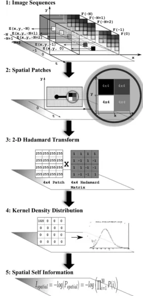
Fig. 3: Spatial Saliency Algorithm Illustration. The algorithm includes following five steps:
1. Getting the present frame Ft=0
2. Patching Ft=0 into E(x, y, 0), ..., Esn(xn, yn,0)
3. Hadamard transforming a square (4x4) patch,
4. Estimating the probability by Kernel Distrubtion Estimation, 5. Calculating self-information wrt Shannon’s theory
From the spatial PDF - figure 2, only the first 30 probability values are preserved for later calculation on account of the assumption that almost all vital information is located near the pdf origin. Then, the probability of an individual patch
P(E) is the production of those 30 probabilities values.
P(E) =
30
Y
i=1
Pi (9)
With the above procedure, the probabilites of any spatial patches can be computed, which in turn lead to the probability of the patches given the spatial context in accord with equation 7.
C. Temporal Saliency Computational Method
As an event E(x, y, t) evolves over time, its information is radically affected by temporal context. Due to assumptions made in the sub-section II-A, temporal information is sep-arated from its general spatial-temporal context. Generally, that information depends on probability of an event E(x, y, t) given the spatial context Vx,y, and the probability is written
as follows.
P(E|Vx,y) =
P(E ∩ Vx,y)
P(Vx,y)
(10)
As Vx,y set includes a record of the event in previous frames
and in the present itself; therefore, the numerator of equation ends up:
P(E ∩ Vx,y) = P (E) (11)
Again, the numerator is the probability of individual patch which can be calculated by procedures mentioned in the subsection II-B; then, only left is the task of figuring out the probability of temporal contexts. Vx,yis a 3-D matrix in which
the evolution of an event in a fixed location(x, y) is recorded from the previous m frame to the present frame. Supposed that each patch has 4x4 size, the probability P(Vx,y) needs
be estimated from a 4x4xm dimensional space. Fortunately, probability estimation of multidimensional spaces has been discussed in the previous section. So the same procedure can be deployed for the temporal probability case except 3-D Hadamard transform is used in the place of its 2-D version. The 3-D Hadamard transform is in fact a combination of one time 2-D transform along its any two dimensions and one time 1-D transform along the other dimension, for example Hx,y,t3D (Vx,y) = Ht1D(Hx,y2D(Vx,y)). The result of
3-D Hadamard transform is later used to estimate probability distribution function shown in the figure 4.
0 10 20 30 40 50 60 70 80 90 100 0 0.2 0.4 0.6 0.8 1 1.2 1.4 1.6x 10
−3Temporal Probability Distribution Function
First 30 probability
values
Fig. 4: Temporal Probability Distribution Function Plot.
Similar to the procedure in the subsection II-B, only first 30 probability values in the pdf are used for calculating P(Vx,y).
2: Temporal Patches y 4x4 4x4 4x4 4x4 4x4 3: 3-D Hadamard Transform 255 255 255 255 255 255 255 255 255 255 255 255 255 255 255 255
Fig. 5: Temporal Saliency Algorithm Illustration. The algo-rithm includes following five steps:
1. Getting the present frame Vx,y
2. Patching Vx,y into Et0(x, y, t0), ..., Etm(x, y, tm) 3. 3D Hadamard transforming a (4x4x5) patch,
4. Estimating the probability by Kernel Distribution Estima-tion,
5. Calculating self-information with respect to Shannon’s theory P(Vx,y) = 30 Y i=1 Pi (12)
D. Spatial-Temporal Saliency Computational Method From the equation 3 and 1, the spatial-temporal saliency scores are computed as follows.
ST S(x, y, t) = −log(P (|Vx,y∩ Ft)
= −log(P (E|Ft)P (E|Vx,y))
= −log(P (E|Ft)) − log(P (E|Vx,y))
= Ss+ St (13)
where Ss and St consecutively represent saliency scores, or
the amount of information, of a specific patch at (x, y, t). As seen in 13, the spatial-temporal saliency score is the sum of two independently derived saliency values in spatial and temporal contexts. Though they are computed separately like in other saliency approaches for simplification, these values are logically fused together by joint probability in natural mathematical ways.
III. SPATIAL-TEMPORALSALIENCYEVALUATION
Even though our saliency model is developed on mathe-matical derivation of strongly established information theory instead of other heuristic ways, there is a need for the method to be evaluated carefully before any further conclusion. For the saliency model relying on space and time, two evaluation test need to be done at least.
First test is conducted to find out how spatial features such as intensity, contrast act upon spatial saliency scores. In this test, predefined matrix is fed into the procedure in the section II-B. In the matrix, there are
1 1 1 1 1 1 255 255 255 255 255 255 2 2 2 2 2 2 255 255 255 255 255 255 .. . ... ... ... ... ... ... ... ... ... ... ... 254 254 254 254 254 254 254 254 254 254 254 254 255 255 255 255 255 255 255 255 255 255 255 255
The above matrix can be seen as an image as well, figure 6. It includes three main columns which are different in patterns. The first column has its intensity increasing from 1 to 255. The third column has a fixed intensity value, 255. Finally, the second column is the hybrid of column 1 and column 3. The spatial saliency scores of those three columns are plotted in figure 7. The curve Column 1 shows the proportional relation between saliency value and spatial saliency scores. Simply, it means the more bright a pixel is, the more salient it is. Then, another relation between contrast and saliency is addressed in the curve Column 2. Decreasing contrast in column 2 of the input image 6 leads the decreasing curve Column 2 in the figure 7. Therefore, saliency scores are proportional to how contrast patches are.
The second evaluation test is carried out to trace response of temporal saliency score due to difference in moving direc-tion. Similar to the first test, the input data and images are predefined and shown in the following pictures.
X: 9 Y: 975 Index: 255 RGB: 1, 1, 1
Test 19 − Input Image
Columns Intensity 1 2 3 0 50 100 150 200 250 300 Column 3 Column 1 Intensity Value (0 − 255) Column 2
Fig. 6: Evaluation Test 1 - Input Image. Including three columns:
+ Column 1: intensity values increasing from 1 to 255 + Column 2: combination of half of column 1 and column 3 + Column 3: intensity values fixed at 255
0 50 100 150 200 250 300 100 150 200 250 300 350 Row Saliency Value
Saliency Response of Three Columns
Column 1 Column 2 Column 3
Convergent Point
Fig. 7: Evaluation Test 1 - Output Image. Including three lines: + Column 1: increasing intensity vs saliency score
+ Column 2: decreasing contrast vs saliency score + Column 3: fixed intensity vs saliency score
a. Right to Left b. Left to Right
c. Bottom to Top d. Top to Bottom
Fig. 8: Evaluation Test 2 - Moving patterns
In this saliency model, saliency responses to motion features are varied; their values are inconsistent with the same amount of movement in different directions. For example, the white bar moving from right to left, figure 8a, in the patch, has saliency score -5.8552, while the same bar, figure 8b, moving in the opposite direction causes saliency value 57.3793.
An-other example is the bar moving from top to bottom and from bottom to top leads to different saliency values 68.7315 and 5.4970 consecutively.
The usage of Hadamard transform may initiate incongru-ous saliency values with respect to movements in different directions. So as to improve the algorithm, several other transform need being examined and hopefully an appropriate transform can be found in terms of both speed and consistency. Moreover, current 3-D Hadamard transform, a combination between 2-D and 1-D Hadamard transform, can be replaced by a direct 3-D Hadamard transform [10]
IV. INFORMATIONVISUALSALIENCYRESULTS Albeit there are still minor flaws in the proposed informatic visual saliency model, it has several vision-based applications. Purposely tailored for spatial and temporal contexts, the model can be deployed in systems in which the input images are videos or continuous images. In addition, it provides essential scene-analyzed information which may highly correlate to human visual attention. This is a widely requested feature in modern intelligent systems;for example, advanced driving assistance systems (ADAS) and video content analysis. Fol-lowing are two samples which demonstrates performance of this information saliency computational method.
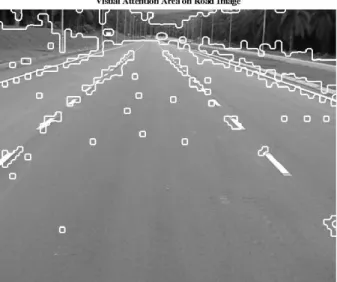
Fig. 9: Visual Attention Regions in A Road Image
In figure 9 is a scene taken in a video from UNMC-VIER Audio-Visual Database [11]. The discrete lane-marks are detected quite well though the program is not intentionally built for that purpose. Other objects on roads such as vehicles and traffic signs could be detected along with lane-marks as well. Perhaps, the model may provide a solution for multi-tasks ADAS. Beside the specific intelligent application like ADAS, the model may contribute into video content analysis, an active academic research field. In this kind of researches, the usual question is which regions on a video scene, for example figure 10, are semantic, and our saliency model can provide saliency map as clues for answering the question.
Fig. 10: Visual Attention Regions in A Game Image
V. CONCLUSION
In this paper, the spatial-temporal saliency approach based on Shannon’s theory is revised and evaluated. Different from many currently popular saliency methods which are heuristi-cally developed, the proposed model is derived in an elegant and concise way. Mathematically, it is a combination between spatial and temporal saliency by their joint probability. More-over, with basic assumptions is simplified the model, so it is tractable in full-motion video processing. Besides that, two simulations have been done to verify how it responds different in spacial and temporal domain. They show that the algorithm can be improved by appropriate choice of transformation technique.
REFERENCES
[1] L. Itti, C. Koch, and E. Niebur, “A model of saliency-based visual at-tention for rapid scene analysis,” IEEE Transactions on pattern analysis
and machine intelligence, vol. 20, no. 11, pp. 1254–1259, 1998.
[2] N. D. B. Bruce, “Features that draw visual attention : an information theoretic perspective,” Neurocomputing, vol. 66, pp. 125–133, 2005. [3] T. Kadir and M. Brady, “Saliency , Scale and Image Description,” Image
(Rochester, N.Y.), pp. 1–45, 2000.
[4] C. L. Guo, Q. Ma, and L. M. Zhang, Spatio-temporal Saliency detection
using phase spectrum of quaternion fourier transform. IEEE, 2008.
[5] Y. Ma, L. Lu, H. Zhang, and M. Li, “A user attention model for video summarization,” in Proceedings of the tenth ACM international
conference on Multimedia, p. 542, ACM, 2002.
[6] Y. Zhai, “Visual Attention Detection in Video Sequences Using Spa-tiotemporal Cues Categories and Subject Descriptors,” Image (Rochester,
N.Y.), vol. 32816.
[7] C. Guo and L. Zhang, “A novel multiresolution spatiotemporal saliency detection model and its applications in image and video compression.,”
IEEE transactions on image processing : a publication of the IEEE Signal Processing Society, vol. 19, no. 1, pp. 185–98, 2010.
[8] T. Topper, Selection mechanisms in human and machine vision. PhD thesis, University of Waterloo, 1991.
[9] G. Qiu, X. Gu, Z. Chen, Q. Chen, and C. Wang, “An information theo-retic model of spatiotemporal visual saliency,” in to appear, international
conference on multimedia and expo, pp. 1806–1809, Citeseer, 2007.
[10] S. S. Adams, M. Crawford, C. Greeley, B. Lee, and M. K. Murugan, “Multilevel and multidimensional Hadamard matrices,” Designs, Codes
and Cryptography, vol. 51, pp. 245–252, Dec. 2008.