數位相機之影像處理: 自動白平衡, 自動曝光, 自動聚焦

行政院國家科學委員會專題研究計畫 成果報告

數位相機之影像處理: 自動白平衡, 自動曝光, 自動聚焦

計畫類別： 個別型計畫

計畫編號： NSC92-2213-E-002-072-

執行期間： 92 年 08 月 01 日至 93 年 07 月 31 日

執行單位： 國立臺灣大學資訊工程學系暨研究所

計畫主持人： 傅楸善

計畫參與人員： 黃柏青, 朱峻賢, 徐中昱

報告類型： 精簡報告

報告附件： 出席國際會議研究心得報告及發表論文

處理方式： 本計畫可公開查詢

中 華 民 國 93 年 8 月 4 日

行政院國家科學委員會專題研究計畫成果報告

數位相機之影像處理: 自動白平衡, 自動曝光, 自動聚焦

Image Processing for Digital Cameras: Auto White Balance, Auto

Exposure, Auto Focus

計畫編號：NSC 92-2213-E-002 -072-

執行期限：92 年 8 月 1 日至 93 年 7 月 31 日

主持人：傅楸善 台灣大學資訊工程系

一、中文摘要

本計畫為期三年、目的是研究利用電

腦視覺與數位影像處理方法，進行數位相

機自動白平衡、自動曝光、自動聚焦之研

究。在計畫執行期間，我們將探討最佳的

攝影機與光源和環境及景物的互動，第一

年研究最佳色彩反應之自動白平衡方法;

第二年控制最適當的光圈大小及快門速度

並且考慮閃光燈的影響以完成自動曝光;

第三年研究各種聚焦感測模組及方法, 以發

展自動聚焦程式及演算法。以突破日本及

美國在這三方面的專利及技術障礙, 提高我

國的數位靜態相機及視訊攝影機在國際巿

場的競爭力。

關鍵詞：自動白平衡、自動曝光、自動聚

焦、電腦視覺、數位影像處理

Abstract

This is a three-year project to use computer vision and digital image processing methods for auto white balance, auto exposure, and auto focus of digital cameras. We will study the best camera, light source, environment, and scene interaction. In the first year, we will develop the auto white balance method for

optimum color response. In the second year, we will control the optimum aperture size and shutter speed and the influence of flash to achieve auto exposure. In the third year, we will research various auto focus sensing modules and methods to develop programs and algorithms for auto focus. We would like to break the patent and technology barriers of Japanese and American companies and to enhance and

competitiveness of Taiwan companies in international markets.

Keywords: Auto White Balance, Auto

Exposure, Auto Focus, Computer Vision,

Digital Image Processing

二、緣由與目的

數位靜態相機 (Digital Still Camera) 及

視訊攝影機 (Digital Video Camcorder) 將大

部份取代現有的軟片相機。相機是很大的

巿場, 國外在美國有柯達 (Kodak); 日本有

Nikon, Canon, Minolta, Sony, Panasonic,

Fujifilm, Konica, … 等; 歐洲有 Leica, Zeiss,

Hasselblad, Agfa, … 等。台灣只要在數位

相機方面佔一席之地, 可以造就出像柯達的

國際大廠。

數位相機目前用的感應器在中低階大

部 份 用 的 是 互 補 式 金 屬 氧 化 物 半 導 體

(CMOS: Complementary Metal Oxide

Semiconductor), 高階相機則大部份用電荷

耦 合 裝 置

(CCD: Charge-Coupled Device)

[26]。 國內已有廠商發展到兩百萬像素

CMOS 感應器, CCD 感應器則全部操縱在

美日廠商的手上。國內如凌暘, 聯詠…等廠

商, 已發展出 Sunplus 533 等數位靜態相機

使 用 的 數 位 處 理 器

(DSP: Digital Signal

Processing) 晶片, 可以和美國德州儀器的

TMS320DSC25 或以色列 Zoran 的 COACH

(Camera On A Chip) 競爭。其中最關鍵的

技術就是自動白平衡, 自動曝光, 自動聚焦

等技術。

國外史丹福大學有一個很大的可程式

數位相機計畫 (Programmble Digital Camera

Project, http://isl.stanford.edu/~abbas/group/)

有 Canon, Kodak, Hewlett-Packard, Agilent

Technolgies 等工業界合作廠商。本實驗室

希望能與他們並駕齊驅, 目前已和傑霖科技,

智基科技, 英華達合作; 而且正在和原相科

技, 聯詠科技…等恰談合作細節中。

第一年我們將研究自動白平衡。自動

白平衡的目標是希望白色即使在不同的光

源下仍然保有原來的白 [33]; 也就是說, 即

使在低色溫的鎢絲燈 (2800 Kelvin) 或蠟燭

光下, 也不會偏黃或紅; 即使在高色溫的日

光燈

(9000 Kelvin) 下也不會偏藍或紫色

[50]。換句話說, 希望在不同光源的頻譜功

率分佈 (SPD: Spectral Power Distribution)

下, 各種顏色仍保有原來的顏色, 而不會變

色。希望達到人類視覺的色彩不變 (Color

Constancy) 的功能 [51]。自動白平衡和色

彩 空 間 的 轉 換

, 色 彩 學 , 色 彩 外 觀 模 型

(Color Appearance Model), 和色彩管理等都

有密切的關係 [1, 2, 15, 16, 20, 53]。

目前自動白平衡最常用的就是灰色世

界假設 (Gray World Assumption) [6], 固然

這是一個合理的假設, 因為在大部份的室內

及室外場景及影片中每個像素平均起來固

然是灰色的, 而且反射率在 18%, 這也就是

為什麼柯達的灰卡常用來幫助手動白平衡

與測光。但是這個假設有很大的缺點, 有時

場景可能大部份是鮮艷的紅色, 則灰色世界

假設會把它調成灰色。如何在合理的灰色

世界假設下, 辨識出不適用的狀況, 並且適

當因應, 是我們研究的方向之一。

另一個常用的假設是完美反射物假設

(Perfect Reflector Assumption) [19], 它假設

影像中最亮的像素是景物中的光滑鏡面反

射所造成的, 所以它應該反映出光源的頻譜

功率分佈, 我們可以根據它執行白平衡, 將

色彩修正成為原來的顏色。但是這個方法

也有它的缺點, 照片中最亮的部份未必就是

完美光滑反射所造成的, 可能是它本身是粗

糙的 (Diffuse), 但是很亮; 也有可能反射不

是完美的, 也許反射本身帶有物體原來的顏

色…等。如何在合理的完美反射物假設下,

辨識出不適用的狀況, 並且適當因應, 是我

們另一個重要的研究方向。

目前自動白平衡很常用的測試工具是

GretagMacbeth ColorChecker, 它包含四列

六行的色塊, 最下面列是白色, 漸暗的灰色,

到黑色; 第三列則包含加色 (Additive Color)

的三主色: 紅綠藍 (RGB: Red, Green, Blue)

和減色 (Subtractive Color) 的三主色: 綠藍,

洋紅, 黃 (CMY: Cyan, Magenta, Yellow), 其

他包括自然的顏色, 例如: 皮膚色, 天空的

藍, 葉子的綠…等。

將 來 驗 證 自 動 白 平 衡 的 程 式 性 能 時

[44], 我們希望定義出數量化的客觀衡量標

準, 例如, 可以將照片由 RGB 色彩空間轉

換到 YCbCr 空間, 計算最下面六塊灰色塊

的每個像素的 的和。因為理想上, 最下面

的六塊灰色塊的每個像素不應該偏紅或偏

藍, 所以它們的

和 都應該是 0, 因此

它們的

和應該是

0, 所以我們希望能

找 出 最 適 當 的 自 動 白 平 衡 演 算 法

, 它的

和可以是最小。定義其他適當的自

動白平衡數量化的客觀衡量標準, 也是我們

的研究方向的一部份。

專業的攝影師在攝影時往往會用濾光

片 (Filter), 濾光片往往會改變場景的顏色,

此時如何做好白平衡是我們重要的研究課

題 [31, 32] 。

我們執行自動白平衡研究時, 將嘗試分

成三個單元與階段: 白點偵測單元 [14], 白

平衡判斷單元, 白平衡調整單元。白點偵測

單元將試著找出照片中的白物品的像素, 換

句話說, 想找出可以代表光源頻譜功率分佈

的像素, 在白平衡調整單元, 據以將白像素

調回真正的參考白, 不偏紅也不偏藍。有時

照片中根本没有白像素, 例如: 相機近拍紅

色的聖誕紅的紅葉

; 這時白平衡判斷單元

可能下決定根本不要執行白平衡, 否則會把

鮮艷的紅葉平衡為灰色。

三、結果與討論

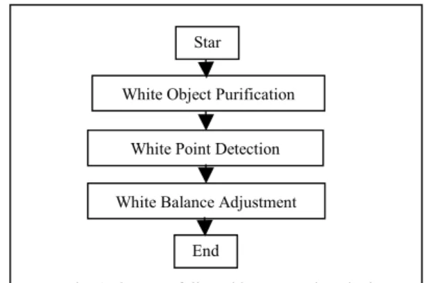
我們的方法包括三步驟: 白物件純化

(White Object Purification), 白 點 偵 測

(White Point Detection), 白平衡調整 (White

Balance Adjustment). 詳細細節請見我們發

表在 IPPR CVGIP 2004 的論文及碩士論文

[54, 55].

白 物 件 純 化 步 驟 把 白 物 件 的 色 偏 移

除。在紅綠藍 (RGB) 三個頻道分別作亮度

長條圖等化 (Histogram Equalization), 可以

把白物件的色偏移除。此步驟之後白點偵

測變成比較容易。

在白點偵測步驟, 我們把亮度長條圖等

化的影像轉化到 YCrCb 色彩空間, 找出可

能是白點的像素並計算它們的平均。如果

找不到可能是白點的像素, 則停止白平衡。

在白平衡調整步驟, 紅綠藍的調整倍數

由參考白點的三個頻道分別計算而得, 並且

判斷該圖的色偏是偏紅, 偏綠, 還是偏藍, 然

後隨之調整。

我們的實驗用各式各樣的光源: 白天

(Daylight), 冷白光 (Cool White), TL84, 白熾

燈

A (Incandescent A), 地平線 (Horizon, 朝

陽或夕陽) 等, 在各式各樣戶內及戶外場景,

用客觀條件和主觀判斷來比較, 我們的方法

在大部份的狀況下, 比其他方法都有較佳的

表現。

四、成果自評

1. 自動白平衡系統之設計流程與參數

設定。

2. 自動白平衡與色彩分析與處理程

式。

3. 結案報告。

4. 詳細報告請見附件論文發表於 CVGIP

2004 及碩士論文 [54, 55].

五、參考文獻

[1] R. M. Adams II and J. B. Weisberg,

The GATF Practical Guide to Color

Management, GATF, Pittsburgh, PA,

1998.

[2] R. S. Berns, Billmeyer and Saltzman’s

Principles of Color Technology, 3

Ed.,

Wiley, New York, 2000.

[3] J.

Bidner,

The Lighting Cookbook,

Amphoto, New York, 1997.

[4] P.

Braczko,

Complete Nikon System:

An Illustrated Equipment Guide, Silver

Pixel Press, Rochester, NY, 2000.

[5] R.

Caputo,

National Geographic

Photography Field Guide: People &

Portraits, National Geographic,

Washington, D.C. 2002.

[6] Y. C. Cheng, W. H. Chan, and Y. Q.

Chen, “Automatic White Balance for

Digital Still Camera,” IEEE

Transactions on Consumer Electronics,

Vol. 41, pp. 460-466, 1995.

[7] D. Cohen, “Automatic Focus Control:

The Astigmatic Lens Approach,”

Applied Optics, Vol. 23, p. 565, 1984.

[8] G. Crawley, “Canon Autofocus Zoom,”

British Journal of Photography, Vol.

128, p. 804, 1981.

[9] G. Crawley, “Canon

EOS-1---Predictive Autofocus,” British Journal

of Photography, Vol. 137, pp. 13-15,

1990.

[10] G. Crawley, “Minolta Dynax

9xi---Predictive Autofocus,” British Journal

of Photography, Vol. 139, p. 19, 1992.

[11] P. Davis, Beyond the Zone System, 4

Ed., Focal Press, Boston, 1999.

[12] I. Davydkin, “Solving the Exposure

Measurement Proglem in

Photography,” Soviet Journal of

Optical Technology, Vol. 48, p. 113,

1981.

[13] H. Denstman, “Autofocus

Technologies,” Professional

Photographer, Vol. 20, No. 9, p. 92,

1980.

[14] A. V. Durg and O. Rashkovskiy,

“Global White Point Detection and

White Balance for Color Images,” U.S.

Patent #6069972, 2000.

[15] L. Eiseman, Pantone Guide to

Communicating with Color, Grafix

Press, 2000.

[16] M. D. Fairchild, Color Appearance

Models, Addison Wesley, Reading, MA,

1998.

[17] B.Farzad, The Confused

Photographer’s Guide to On-Camera

Spotmetering, Confused Photographer’s

Guide Books, Birmingham, AL, 2001.

[18] B.Farzad, The Confused

Photographer’s Guide to Photographic

Exposure and the Simplified Zone

System, Confused Photographer’s

Guide Books, Birmingham, AL, 2001.

[19] M. Fedor, “Approaches to Color

Project, Department of Psychology,

Stanford University, 1998.

[20] E. J. Giorgianni and T. E. Madden,

Digital Color Management: Encoding

Solutions, Addison Wesley, Reading,

MA, 1998.

[21] N. Goldberg, “Inside Autofocus,”

Popular Photography, Vol. 89, No. 2, p.

77, 1982.

[22] C. Graves, The Zone System for 35mm

Photographers, 2

Ed., Focal Press,

Boston, 1997.

[23] R. Hicks and F. Schultz, Learning to

Light: A Practical Guide to

Photographic Lighting for the Amateur,

Amphoto, New York, 1998.

[24] T. Hogan, Nikon Flash Guide, Silver

Press, Rochester, NY, 2001.

[25] J. Holm, “A System for Exposure

Determination and Tone Reproduction

Control in Black and White

Photography,” Kodak Tech Bits, No. 3,

23-28, 1990.

[26] G. C. Holst, CCD Arrays, Cameras,

and Displays, 2

Ed., JCD Publishing,

Winter Park, FL, 1998.

[27] C. Johnson, The Practical Zone System,

3

Ed., Focal Press, Boston, 1999.

[28] K. Kazuo, “Light Measuring System for

Minolta 9000,” Minolta Techno Report

Special, pp. 85-91, 1986.

[29] H. Koch and K. Gfeller, “Selective

Exposure Control for Large Format

Still Cameras,” Journal of Imaging

Technology, Vol. 10, p. 87, 1984.

[30] E. Kodak Company, Kodak Gray Cards,

Silver Pixel Press, Rochester, NY, 1999.

[31] E. Kodak Company, Kodak

Photographic Filters Handbook,

Eastman Kodak, Rochester, NY, 1990.

[32] E. Kodak Company, Using Filters (The

Kodak Workshop Series), Silver Pixel

Press, Rochester, NY, 2002.

[33] M. Y. Lu and P. B. Denyer, “Method

and Apparatus for Controlling Color

Balance of a Video Signal,” U.S. Patent

#5504524, 1994.

[34] A. Mannheim, “Pentax ME-F TTL

Autofocus,” British Journal of

Photography, Vol. 128, p. 1214, 1981.

[35] H. Masataka and N. Toshio,

“Autofocus Technology for Minolta,”

Minolta Techno Report, No. 6, pp.

36-44, 1989.

[36] R. Mitkin and V. Karpushin,

“Automatic Camera Lens Focusing

Systems,” Soviet Journal of Optical

Technology, Vol. 49, p. 453, 1982.

[37] N. Motohiro and M. Yukari,

“Multi-Beam Autofocus,” Minolta Techno

Report, No. 6, pp. 45-52, 1989.

[38] M. Motonobu, “Autofocus with a

Position Sensor Applying

‘Cross-Talk’,” Minolta Techno Report, No. 1,

pp. 22-29, 1984.

[39] F. Patterson, Photography and the Art

of Seeing, Key Porter, Toronto, 1989.

[40] B. Peterson, Understanding Exposure,

Amphoto, New York, 1990.

[41] B. M. Peterson, Magic Lantern Guide

to Nikon Lenses, 2

Ed., Silver Pixel

Press, Rochester, NY, 2000.

[42] S. F. Ray, Applied Photographic Optics,

3

Ed., Focal Press, Oxford, 2002.

[43] S. F. Ray, Scientific Photography and

Applied Imaging, Focal Press, Oxford,

1999.

[44] K. Taniguehi and K. Kanamori,

“Apparatus for Calculating a Degree of

White Balance Adjustment for a

Picture,” U.S. Patent #5619347, 1997.

[45] K. Toshihiko, “AF Sensor Module,”

Minolta Techno Report Special, pp.

40-48, 1986.

[46] M. Uno, “A CMOS Linear Image

Sensor for Passive Autofocusing

Systems,” Journal of Society of

Photographic Science and Technology

Japan, Vol. 60, pp. 98-102, 1997.

[47] G. Wakefield, “Spot Metering,” British

Journal of Photography, Vol. 134, p.

1071, 1987.

[48] G. Wakefield, “The Weston Exposure

Meter,” British Journal of Photography,

Vol. 137, pp. 16-17, 1990.

[49] G. Wakefield, “Gossen Spot-Master,”

British Journal of Photography, Vol.

140, p. 27.

[50] G. Wakefield, “Color Temperature and

a Modern Meter,” British Journal of

Photography, Vol. 135, pp. 10-11,

[51] B. A. Wandell, Foundations of Vision,

Sinauer, Sunderland, MA, 1995.

[52] E. Wildi, Photographic Lenses,

Amherst Media, 2001.

[53] G. Wyszecki and W. S. Stiles, Color

Science: Concepts and Methods,

Quantitative Data and Formulae, 2

Ed., Wiley, New York, 2000.

[54] V. Chikane and C. S. Fuh, “Automatic

White Balance for Digital Still

Camera,”

Proceedings of IPPR

Conference on Computer Vision,

Graphics, and Image Processing,

Hua-Lien, 2004.

[55] V. Chikane, “Automatic White Balance

for Digital Still Camera,” Master

Thesis, Department of Computer

Science and Information Engineering,

National Taiwan University, 2004.

附件：封面格式

行政院國家科學委員會補助專題研究計畫成果報告

※※※※※※※※※※※※※※※※※※※※※※※※※※※

※

※

數位相機之影像處理: 自動白平衡, 自動曝光, 自動聚焦

※

※ ※

※※※※※※※※※※※※※※※※※※※※※※※※※※

計畫類別：■個別型計畫 □整合型計畫

計畫編號：NSC 92-2212-E-002 -072-

執行期間：

92 年 8 月 1 日至 93 年 7 月 31 日

計畫主持人：傅楸善 (台灣大學資訊工程系)

共同主持人：

計畫參與人員：黃柏青, 朱峻賢, 徐中昱

本成果報告包括以下應繳交之附件：

□赴國外出差或研習心得報告一份

□赴大陸地區出差或研習心得報告一份

V 出席國際學術會議心得報告及發表之論文各一份

□國際合作研究計畫國外研究報告書一份

執行單位：台灣大學資訊工程系

中 華 民 國 93 年 8 月 2 日

AUTOMATIC WHITE BALANCE FOR DIGITAL STILL CAMERA

Varsha Chikane and Chiou-Shann Fuh (

傅楸善

)

Department of Computer Science and Information Engineering,

National Taiwan University, Taipei, Taiwan.

ABSTRACT

In recent years digital cameras captured the camera market. Although quality and quantity factors are considered, consumers are more nostalgic about the quality of the picture. White balance is one of the factors used to improve the quality of the picture. The basic white balance methods are powerless to handle all possible situations in the captured scene. In order to improve the white balance we divide this problem in three steps–white object purification, white point detection, and white point adjustment. The proposed method basically solves the problem of detecting white point very well. The experimental results show the proposed method has the best result in both objective and subjective evaluative results. The complexity of the proposed system is acceptable. The proposed method 1 can be easily applied to the digital cameras to get good effects.

Keyword: white balance, gray world assumption, perfect reflector assumption.

1. INTRODUCTION

Whenever the scene is captured by digital camera, every pixel value of the recorded scene depends upon the 3-sensors response and the 3-sensor response is affected by the illuminant of that scene. As an effect the distinct color cast appears over the captured scene. Such effect of the light source appears on the recorded image due to color temperature of the corresponding light source. When a white object is illuminated with low color temperature light source, the object in the captured image will have reddish color. Similarly, if the white object is illuminated with high color temperature light source, the object in the captured image will have a bluish color. For developing white balance algorithm it

This research was supported by the National Science Council of Taiwan, R.O.C., under Grants NSC 92-2213-E-002-072, by the EeRise Corporation, EeVision Corporation, Machvision, Tekom Technologies, Jeilin Technology, IAC, ATM Electronic, Primax Electronics, Arima Computer, and Lite-on.

is necessary to render the information about the illuminant of the scene.

The human vision may not be able to distinguish the color difference caused by various light sources due to the “color constancy” of human eye [1]. Colors remain constant through recognition despite they are viewed under different light sources. In summary, the mechanism employed in digital camera to compensate the color difference caused by various light sources is white balance. This is the main investigation.

2. BACKGROUND

The traditional methods used to adjust the white balance automatically are mentioned below,

2.1. Gray World Method (GWM)

Gray world assumption [2] states that, given an image with sufficient amount of color variations, the average value of the RED, GREEN, and BLUE components of the image should average out to a common gray-value. With gray world assumption, the average of the reflectance of the visible surfaces in every scene is assumed to be gray to estimate the spectral distribution of the illuminant

.

2.2. Perfect Reflector Method (PRM)

In perfect reflector assumption [4], it is considered that the RGB values of the “brightest" pixel in an image captured by digital camera, is the glossy or specular surface. For any white balancing algorithm, it is most important to gather information about surfaces in the scene as well as illuminant of the scene. PRA focuses on both of these facts by underlining the presence of “specularity” or glossy surfaces in an image. The specularity is helpful to convey a good amount of information about the illuminant. Specularities or glossy surfaces reflect the actual color of the light source because these specularities have reflectance functions that are constant over a wide range of wavelengths. By detecting such specularities it is easy to find out the actual color of the light source which is further used to eliminate influence of illuminant over the scene. This

method exploits the perfect reflector assumption to correct the image. It locates the reference white point by finding the pixel with the greatest luminance value and performs the white balance adjustment according to the reference white point.

2.3. Fuzzy Rules Method (FRM)

In FRM [3] the image is converted from the RGB color space to the YCrCb color space and seized the color’s

characteristics in the YCrCb color space for the white

balance adjustment. Image is divided into 8 segments for more precise white balancing.

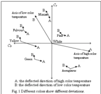
The experimental results shown in Fig.1 are:

1. A dark color has less deviation from nominal position under different light sources, as opposed to the bright color,

where the deviation is

2. When a white color is illuminated with different light sources, the ratio of Cr

to Cb will be approximately between

-1.5 to -0.5.

3. At high luminance, the color components are easy to be saturated; while at low luminance, the color components become colorless.

The fuzzy rules based on experimental results are described below:

1. The averages of Cr and Cb for each

segment will be weighted with small values under the conditions of high-end and low-high-end luminance in order to avoid being saturated and colorless. 2. The averages of Cr and Cb for each

segment are weighted less for dark colors than bright colors.

3. When a large object or background occupies more than one segment, its color will dominate that segment. The ratio of Cr to Cb will be similar among

adjacent segments. The given weighting for those segments having a uniform chromatic color is small in order to avoid over-compensation on the color of the picture.

If the ratio of Cr to Cb for the segment is approximately

between –1.5 to –0.5, the probability of being a white region increases, the given weighting is the largest. Besides these basic methods another method is chiou’s white balance [6] method which tries to overcome the drawbacks of the basic methods.

2.4. Chiou’s White Balance Method (CWBM)

The component block diagram of CWBM is shown in Fig.2.

2.4.1. White point detecting unit

In this unit the reference white points are detected. First the rough reference white pixels are detected. Convert the image from RGB color space to the YCrCb color

space. Next pick up the pixels satisfying the Equation 1.1.

th b

r C CH

C2+ 2≤ (1.1)

where, threshold CHth is equal to 60 in the experiment

and 2 2

b r C

C + be the chromaticity value. Second, select

the pixels among the rough reference white pixels satisfying the Equation 1.2 as precise reference white pixels.

(1.2) where, Rth , Gth , and Bth are threshold picked up from

eightieth percentile of each component histogram. ABr

(= 45), ABb (= 45) are the absolute values of Cr, Cb

respectively. Rl (= - 1.25), Ru (= - 0.75) are lower and

upper range for ratio of Cr to Cb. Finally the averages of

rough reference white pixels and precise reference white

Star

White Point Detecting Unit White Balance Judging Unit White Balance Adjusting Unit

End

Fig. 2 The component block diagram of CWBM u b r l b b r r th th th

R

C

C

R

AB

C

AB

C

B

B

G

G

R

R

≤

≤

≤

≤

≥

≥

≥

,

,

,

pixels are calculated as (Rr , Gr , Br) and (Rp , Gp , Bp)

respectively.

2.4.2. White balance judging unit

This unit judges whether or not to apply the white balance on the desired image. Pick up the reference white point data from the white point detecting unit. First calculate the Rrough , ratio of rough reference white

pixels to all pixels of the image, and Rprecise, ratio of

precise reference white pixels to all pixels of the image. Second, determine whether Rrough is grater than equal to

Prough, defined as prescribed proportion (0.2 in

experiment) and next determine whether Rprecise is grater

than equal to Pprecise , defined as prescribed proportion

(0.05 in experiment) Finally mode Ma is set to the value

0, 1, or 2 as shown in Fig 3.

2.4.3. White balance adjusting unit

This unit adjusts the white balance according to the mode Ma. First calculate the scale factors according to

rough reference white point (Rrgain, Grgain, Brgain) also

calculate the scale factors according to precise reference white point (Rpgain, Gpgain, Bpgain). If Ma is set to the value

2 then white balance is adjusted according to the (Rpgain,

Gpgain, Bpgain). If Ma is set to the value 1 then select the

minors between (Rrgain, Grgain, Brgain) and (Rpgain, Gpgain,

Bpgain). Next if Ma is set to the value 0 then do not apply

white balance adjustment.

For adjusting the extreme scale factors towards an acceptable values sigmoid function shown in Equation 1.3 is used.

4

.

0

))

25

.

1

tanh(

1

(

*

05

.

1

+

−

+

=

X

Y

3. EXPERIMENTS

Camera used for experiments is set to the raw data mode for avoiding any image processing. The binary color interpolation scheme is applied for getting the RGB image data. For more precise knowledge about the color variations due to different light sources we capture the images of GretagMacbeth ColorChecker in two

categories; varying lighting conditions and varying object conditions. For varying lighting conditions, we capture images of the GretagMacbeth ColorChecker under standard light sources as shown in Table 1 and also capture images of GretagMacbeth ColorChecker under natural and household light sources.

For varying object conditions, images are capture with and without ColorChecker. According to the CWBM and FRM the white points are detected by using predefined values of Cr and Cb. In most of the cases, this

predefined range for Cr and Cb selects another color

pixel as white point. Our main purpose is to use the small range to detect the white points from the desired image. After some experiments and observations, we propose new approach for white balance adjustment.

4. NEW APPROACH FOR WHITE BALANCE

We propose original idea of white object purification step. According to the observations based on experiments, if we purify the white object, then it is easy to detect the white point from the images. For this purpose we apply histogram equalization on the desired image and extract information about the pixels belonging to the white point and then use this information to select the white point from the original image. The new approach for white balance follows the steps as shown in Fig. 4.

4.1 White Object Purification

The first step, white object purification purifies the white object in such a way that the color cast over the white object is removed. Applying histogram equalization on the RGB channel separately results in removing the color cast over the white object. After this step white object detection becomes easier.

Light source

Daylight Cool white

TL84 Inc. A’ Horizon Color

temperature (°K)

6500 4180 4100 2850 2300

Star

White Object Purification White Point Detection White Balance Adjustment

End

Fig. 4 The steps followed in proposed method. No Yes Yes Yes No No rough rough P R ≥ precuse precise P R ≥ Rprecise≥Pprecuse Ma=2 Ma=1 Ma=0

Fig. 3 Conditions for setting mode

The flow chart of the white object purification is shown in Fig. 4.1. First store the original image data. Next apply histogram equalization to each RGB channel separately. For further processing use the Histogram equalize image data in YCrCb color space.

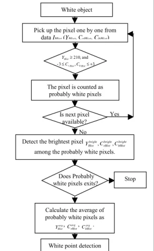
4.2 White Point Detection

In this step, we make use of histogram-equalized image data (YHist, CrHist, CbHist) in YCrCb color space. First,

detect those pixels satisfying Equation 1.4 as probably white pixels and next calculate averages of selected probably white pixels as, avg

Hist

Y

,

,

C . If none of

the probably white pixel is detected then we stop for white balance.

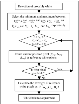
The flow chart of the detection of probably white pixels is shown in Fig. 4.2.1.

Next, find out the brightest pixels

bright bHist bright rHist bright Hist C C

Y , , with maximum YHist value, and CrHist, CbHist values should be closest to zero, among all

probably white pixels. Second, if the pixels, from the histogram-equalized image data satisfy Equation 1.5, then select the corresponding position pixels from the original RGB color space image data as reference white pixels. u b bHist l b u r rHist l r u Hist l

C

C

C

C

C

C

Y

Y

Y

≤

≤

≤

≤

≤

≤

values between bright bHist bright rHist bright Hist C C Y , , and avg Hist Y , avg rHist C , avg bHist

C . Similarly

Y

,

C

,

and

C

maximum values between bright bHist bright rHist bright

Hist C C

Y , , andY_Histavg, avg

rHist

C , CbHistavg . Finally, the average of those reference

white pixels is calculated as reference white point W (Rw,

Gw, Bw). The collected white balance data are transferred

to the white balance adjustment unit. The flowchart of the white point detection is show in Figure 4.2.2.

White point detection Covert image space from RGB to

YCrCb

Store the original image data

Iorg (Rorg, Gorg, Borg) Apply the histogram equalization to Image

Start

Fig. 4.1 Flowchart of white object purification.

Does Probably white pixels exits?

No White object Pick up the pixel one by one from

data IHist(YHist, CrHist, CbHist)

3 , 3 -and , 210 + ≤ ≤ ≥ Hist b Hist r Hist C C Y

The pixel is counted as probably white pixels

Yes Is next pixel

available?

Detect the brightest pixel bright bHist bright rHist bright Hist C C Y , , among the probably white pixels.

Calculate the average of probably white pixels as

avg Hist Y , CavgrHist , avg bHist C .

White point detection

Fig. 4.2.1 Detection of probably white pixels. Stop

4.3 White Balance Adjustment

First, collect the data from the white point detection unit and proceed for white balance adjustment. Second, scale factors are calculated according to the reference white point W ( R_w ,G_w ,B_w) for respective

color component as shown in Equation 1.6.

w w scale w w scale w w scale B Y B G Y G R Y R / / / = = = _(1.6)

where, _{Y is calculated by Equation 1.7. w}

w w

w

w R G B

Y =0.299* +0.587* +0.114* (1.7)

Next the scale factors are calculated according to GWA as shown in Equation 1.8. avg avg GWA avg avg GWA avg avg GWA B Y B G Y G R Y R / / / = = = _(1.8)

Finally decisions are made for selecting proper scale factors based on color cast over the desired image. For determining the color cast over the image, convert the average values of the probably white pixels, avg

Hist Y , avg rHist C , avg bHist

C from RGB to YCrCb color space as avg Hist

R , G_Histavg,

avg Hist

B . Next use Equations from 1.9 to 1.11 to find bluish,

greenish, and reddish color casts respectively. Although these equations are determined based on observation, it is consistent to make use of those equations for finding the color cast over the image.

avg Hist avg Hist avg Hist avg Hist G B R B +3≥ and > (1.9) avg Hist avg Hist avg Hist R B G +3> > (1.10) avg Hist avg Hist avg Hist G B R > > (1.11)

After finding the color cast, the scale factors are applied. In case of bluish cast, the scale factors are selected as shown in Equation 1.12. GWA factor scale factor scale factor B B G G R R = = =

In case of reddish cast the scale factors are selected as shown in Equation 1.13. scale factor scale factor GWA factor B B G G R R = = =

In case of greenish cast the scale factors are selected as shown in Equation 1.14. Scale factor GWA factor scale factor B B G G R R = = =

Those selected scale factors are applies to the whole image in order to get white balanced image. The

No No No Yes Yes Yes 1 = colorcast White point

Calculate the scale factors w w scale w w scale w w scale Y R G Y G B Y B R = / , = / ,and = /

Calculate the color cast

colorcastas 0, 1, 2, or 3. 2 = colorcast 3 = colorcast

Apply the scale factors, GWA factor scale factor scale factor B B G G R R = = = and , ,

Apply the scale factors, scale factor GWA factor scale factor B B G G R R = = = and , ,

Apply the scale factors, scale factor scale factor GWA factor B B G G R R = = = and , , En

Fig. 4.3 Flowchart of white balance adjustment. Calculate the scale factors

avg avg GWA avg avg GWA avg avg GWA Y R G Y G B Y B R = / , = / ,and = / Yes No

Detection of probably white

Select the minimum and maximum between bright bHist bright rHist bright Hist C C Y , , and avg Hist Y , avg rHist C , avg bHist C as l b l r l C C

Y , ,and , Yu ,Cru ,andCburespectively.

u b bHist l b u r rHist l r u Hist l C C C C C C Y Y Y ≤ ≤ ≤ ≤ ≤ ≤

Count current position pixel (Rorg, Gorg,

Borg) as reference white pixels.

Is next pixel available?

Calculate the averages of reference white pixels as W (R_w ,G_w ,B_w)

White balance adjustment

4.2.2 White point detection.

(1.12)

(1.13)

flowchart of the white balance adjustment is shown in Figure 4.3.

5. RESULTS

We captured the test images of GretagMacbeth ColorChecker under five light sources and also under the household light sources. In addition to check stability of proposed method we also capture test images of the same scene with and without ColorChecker. Next apply the white balance method based on basic assumptions and proposed method to the test images. For more precise comparisons between all methods, we calculate the average chromaticity, 2 2

b r C

C + of the

achromatic patches of the ColorChecker as objective evaluative values. Besides the objective evaluation we also ask group of people to choose the best image among the five methods, which they would like. The image of the GretagMacbeth ColorChecker under daylight source and visual results after applying five methods are shown in Fig. 5.

Besides, these the observations under standard light source we also capture images of the ColorChecker under natural light source; sunny climate. The visual results under sunny climate are shown in Fig. 6.

For more precise results we also capture the images with and without ColorChecker in order to test the stability of our method. The visual results with and without ColorChecker are shown in Fig. 7. In Fig. 7 left column resultant images with ColorChecker and right column images are without ColorChecker.

(e) (f) (d) (c)

(b) (a)

Fig. 5 (a) Original image captured under daylight visual results after applying (b) GWM, (c) PRM, (d) FRM, (e) CWBM, (f) Our method. (f) (e) (d) (c) (b) (a)

Fig. 6 (a) Original image- Greenery: captured under cloudy weather visual results after applying (b) GWM, (c) PRM, (d) FRM, (e) CWBM, (f) Our method.

We make the use of average chromaticity value of achromatic patches of the ColorChecker as objective evaluative values, for comparing the all five methods. The method which forces the chromaticity value closer to the zero is said to be best among five methods. Subjective evaluative values are vote of the group of people.

The objective and subjective evaluative values for all test images captured under standard as well as natural and household light sources, are shown in Table 2.

Table 2 Objective and subjective (backed values) evaluative values for all test images

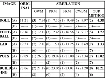
The objective and subjective evaluative values for the test images with and without ColorChecker are shown in Table 3. Note that in Table 3 (B) row of each image is without ColorChecker so chromaticity value for such images is not available so those block are shown by using dotted lines.

6. CONCLUSION

According to the experiments, we find that there are some serious problems with GWM, PRM, FRM, and CWBA. There are some situation where adjusting the white balance destroys the consistency of colors in the image. Therefore, to avoid such situations we make use

SIMULATION IMAGE ORIG--INAL GWM PRM FRM CWBM OUR METHOD (A) 23.47 (4) 1.71(1) 2.06 (0) 15.62 (1) 4.77 (5) 1.71 DAY LIGHT (B) 15.65 (3) 1.26 (0)15.65 (0) 11.15 (3) 9.97(3) 1.36 (A) 16.57 (2) 1.43(1) 1.42 (0) 11.50 (6) 3.68 (3) 1.42 COOL WHITE_{(B) 9.32 (4) 1.71(0) 7.70 (0) 7.04 (2) 6.26 (3) 3.80} (A) 16.35 (7) 1.47(0) 1.42 (0) 11.66 (0) 3.99 (3) 1.29 TL84 (B) 9.61 (5) 1.52(0) 4.99 (0) 10.99 (0) 3.99(5) 3.97 (A) 20.07(3) 1.05(0) 3.44 (0) 14.40 (2) 7.66 (4) 2.08 INC. ‘A’ (B) 10.56(4) 1.01(1) 9.45 (1) 7.60 (2) 5.97 (5) 1.08 (A) 33.19(4) 0.65(0) 8.66 (0) 22.28 (2) 17.26 (4) 0.76 HRZ (B) 19.91(3) 1.57(0) 9.47 (0) 13.36 (3) 9.35 (4) 2.31 GREEN _{20.73 (0) 25.11 (2)20.73 (0) 20.90 (0) 21.18 (7) 9.11} STEPS _{20.09 (1) 16.36 (2) 5.79 (1) 19.28 (4) 17.93 (3) 2.97} CAT _{15.51 (1) 19.34 (1) 6.30 (1) 16.22 (2) 19.38 (6) 2.64} LCD _{10.50 (0) 12.82 (1) 5.00 (0) 11.85 (3) 13.95 (5) 2.50} FOG _{24.62 (1) 15.70 (0)24.62 (0) 16.83 (3) 14.50 (5) 7.93} SIMULATION IMAGE ORIG-INAL GWM PRM FRM CWBM OUR METHOD (A) 11.21 (3) 7.94 (1) 7.10 (1) 9.49 (6) 9.97 (2) 4.38 DOLL (B) --- (1)--- (1)--- (0)--- (7)--- (3)--- (A) 19.16 (1) 12.12 (3) 2.45 (1) 16.56 (3) 9.17(5) 1.72 FOOT-BALL _{(B) --- (2)--- (3)--- (1)--- (3)--- (5)} ---(A) 19.23 (7) 2.10 (0) 15.1 (1) 13.25 (1) 8.69(7) 1.33 LAB (B) --- (6)--- (1)--- (1)--- (1)--- (7) ---(A) 19.09 (1) 26.36 (3) 19.09 (1) 21.00 (3) 23.34(7) 15.02 POTS (B) --- (1)--- (2)--- (1)--- (2)--- (7) ---(A) 23.06 (2) 21.17 (0) 23.06 (1) 23.01 (4) 21.20(8) 10.21 BUILD -ING _{(B) --- (2)--- (0)--- (2)--- (4)---} (6) ---a2 b1 c1 b2 c2 d1 e1 d2 e2 f2 f1 a1

Fig. 7 (a1, a2) Original image- Pots: capture under sunny climate with (a1) and without (a2) ColorChecker. Visual results after applying (b1, b2) GWM, (c1, c2) PRM, (d1, d2) FRM, (e1, e2) CWBM, (f1, f2) Our method.

Table 3 objective and subjective evaluative values for the test images with and without ColorChecker.

of color cast finding equations and some conditions in order to make decision, whether or not to apply white balance adjustment. Sometimes, under the situations such as greenery, applying any white balance algorithm may result in the bluish cast instead of removing the original color cast. In our method we also try to get rid of such situations. Under natural light sources and household lights our method performs the best.

The simulation result shows that, our method has the best performance in both objective as well as subjective evaluation. Experiments performed with and without Macbeth ColorChecker shows, the stability of our method in removing the color cast over the scene under object varying situations. Besides object varying situations we also consider the light varying conditions by capturing the same scene under different light sources the results again remains stable so our method can be applicable for the moving pictures white balance. Consideration of single brightest pixel for white balancing, which is the main drawback of PRM is overcome by our method. Because we make use of some range for finding the brightest pixel, detected brightest pixel always belongs to the white color. Our method works under all possible situations because of the brightest pixel is used for finding the range to detect the white pixels under the color cast. In this way, our method either removes the color cast completely or stops for white balance adjustment. Complexity of proposed method is also acceptable.

Uniqueness of our method is white object purification step and it also opens the new way for the white balance algorithm. Due to the white object purification, the proposed method successfully finds the white object under any color cast as effect of surrounding light source.

7. FUTURE WORK

We are continued to perform the experiments mainly in white object purification unit. Under some rare situations histogram equalization could not do best to purify the white object in the desired image. Another area of improvement is the white balance adjustment, as we observed that the different color shown different color deviations due to the light sources and we are just adjusting the white object properly. If we find some way to apply the scale according to the color then it would be the proper solution for removing the color cast over the all scene colors. Whenever there is no white object present, proposed method does not apply white balance for such scenes. Color cast over the scenes without white objects will not be removed so we will continue to find some solution to solve this problem.

8. REFERENCES

[1] R. C. Gonzalez and R. E. Woods, Digital Image

Processing, Addison Wesley, Reading, MA, 1992.

[2] M. Fedor, “Approaches to Color Balancing,” PSYCH221/EE362course project, Department of Psychology, Stanford University, 1998.

[3] Y. C. Cheng, W. H. Chan, and Y.Q. Chen, “Automatic White Balance for Digital Still Camera,” IEEE Transactions

on Consumer Electronics, Volume 41, pp. 460-466, 1995.

[4] J. Chiang and F. Al-Turkait, “Color Balancing Experiments with the HP-Photo Smart-C30 Digital Camera,” PSYCH221/EE362 course project, Department of Psychology, Stanford University, 1999.

[5] A. V. Durg and O. Rashkovskiy, “Global White Point Detection and White Balance for Color Images,” U.S. Patent #6069972, 2000.

[6] T. S. Chiou, “Automatic White Balance for Digital Still Camera,” Master Thesis, Department of Computer Science and Information Engineering, National Taiwan University, Taiwan, 2000.