美國對台灣股市外溢效果之分量迴歸分析

(1)

國

立

交

通

大

學

經營管理研究所

碩

士

論

文

美國對台灣股市外溢效果之分量迴歸分析

Quantile Regression Analysis of the Spillover Effect of

US-Taiwan Stock Markets

研究生：蔡佳樺

指導教授：周雨田教授

中

中華

華

華民

民

民國

國

國九十八

九十八年

九十八

年

年六

六

六月

月

(2)

美國對台灣股市外溢效果的分量回歸分析

Quantile Regression Analysis of the

Spillover Effect of US-Taiwan Stock

Markets

研究生︰蔡佳樺

Student︰Chia-Hua Tsai

指導教授︰周雨田博士

Advisor︰Dr. Ray Yeu-Tien Chou

國立交通大學

經營管理研究所

碩士論文

A Thesis

Submitted to Institute of Business and Management

College of Management

National Chiao Tung University

in Partial Fulfillment of the Requirements

for the Degree of

Master of Business Administration

June 2009

Taipei, Taiwan, Republic of China

中華民國九十八年六月

(3)

美國對台灣股市外溢效果之分量迴歸分析

學生：蔡佳樺指導教授：周雨田博士

國立交通大學經營管理研究所碩士班

摘摘摘 摘要要要要本篇使用分量迴歸模型 (Quantile Regression) 來探討美國股市對台灣股票市場的外溢效果是否存在，美股以S&P 500為代表，台股則分別取台股加權指數和店頭市場加權指數為代表，並區分為close-to-open, open-to-close和close-to-close三階段報酬來探討，實證結果發現：1. 美股對台股在close-to-open報酬具有外溢效果，此外，透過分量迴歸我們發現1995年到1997年在漲跌幅大時才具有外溢效果。2. 美股對台股在close-to-close 報酬亦具有外溢效果，除了在1995年到1997年，當股價達最大跌幅時，美股對台股不但不具有外溢效果，反而為負向的影響。3.本篇論文證實，美股對台股在open-to-close報酬確實具有過度反應效果，且除了1995年到1997年過度反應效果僅存在於股價漲跌幅極大外，金融海嘯時期，當股價達致最大跌幅則亦不具有過度反應效果。關鍵詞關鍵詞關鍵詞關鍵詞：：：：外溢效果外溢效果外溢效果外溢效果、、過度反應效果、、過度反應效果過度反應效果過度反應效果、、、、普通最小平方法普通最小平方法、普通最小平方法普通最小平方法、、、最小最小最小絕對最小絕對絕對離差絕對離差離差法離差法法法

(4)

Quantile Regression Analysis of the Spillover Effect of US-Taiwan

Stock Markets

Student : Chia-Hus Tsai Advisor : Dr. Ray Yeu-Tien Chou

Institute of Business and Management

National Chiao Tung University

ABSTRACT

This paper employs quantile regression model to investigate if the price change spillover

effect exists from U.S. to Taiwan. We discuss three market segments of Taiwan stock which

comprise close-to-open, open-to-close and close-to-close returns respectively. We find that:

Firstly, the price change spillover effect exists from U.S. to the close-to-open returns of

Taiwan stock market. Furthermore, the price change spillover effect exists when stock price

goes up or down greatly from 1995 to 1997. Secondly, the price change spillover effect exists

from U.S. to the close-to-close returns of Taiwan stock market. However, there is no price

change spillover effect when price goes down greatly and there is even negative effect from

U.S. to Taiwan from 1995 to 1997. Thirdly, the overreaction effect exists from U.S. to the

open-to-close returns of Taiwan except from 1995 to 1997. The overreaction effect only exists

when price goes up or down greatly from 1995 to 1997, and there is no overreaction effect

when price goes down greatly in Financial Tsunami.

Keywords : Spillover effect, Overreaction effect, Ordinary least squares method, Least absolute deviations method

(5)

誌謝

我的研究所生活以及本篇論文能夠順利完成，最感謝的，是我的指導老師－周雨田教授，周老師不但時時給予我建議，也耐心地指導我。在我們面臨不景氣的求職期間，也給予我們很大的空間，讓我們能夠安心地找工作，在找工作和寫論文中取得平衡，這一切都歸功於周雨田教授！此外，初稿的審查委員胡均立所長、丁承教授的意見，另外兩位口試委員林常青、巫春洲教授的指教，都協助了我能夠順利完成此篇論文，學生在此非常感謝。在論文撰寫的期間，學長姐們和同學們之間的幫忙也是最大的助力。感謝致宏學長在當兵時還抽空幫我解答、念青學長從碩一開始對於我選課與論文方向的建議、炳麟學長幫忙我解決 E-Views 上的問題、新風學長提供軟體、孫蕾學姐提供簡報上的指導，周家班的昱如、琬珈、泰佑、信國的彼此打氣、小白提供研究室讓我抓 data、憲堂幫忙我修改圖……等，很多很多的感謝。最後需要感謝我的家人，這兩年來一直支持著我，常常幫我補身體，擔心我的體力不夠，也常常包容我的小任性。對於大家的感謝我會一直放在心中，將此篇論文獻給最親愛的你們！

(6)

摘

摘要

要

要………...i

ABSTRACT………..………...…...ii

誌

誌謝

謝

謝………...iii

Table of Contents……….……….iv

List of Tables……….………...v

List of Figures……….………...…...ix

1. Introduction……….…...…...1

2. Literature Review……….…….…………..…..…...4

2.1 Cross-Market Spillover Effect……….…….….…...…...…..4

2.2 Overreaction Effect……….…..………….…...…...…..6

2.3 Quantile Regression………..…………..…...……...8

3. Data...…………...……….…...11

3.1 Sample………..…..11

3.2 Descriptive Statistics……...……….………...13

4. Estimation Results………...…...15

5. Conclusion………...24

Reference………..………...26

(7)

List of Tables

Table 1: Descriptive Statistics………...…….…27

Table 2: Quantile Regression Result of Close-to-open Returns of TAIEX,

1995-1997………..…...28

1997-2000………..…...29

2000-2007………..…...30

2007-2009……….……...31

1995-2009………....32

Table 7: Quantile Regression Result of Close-to-open Returns of OTC,

1995-1997………....33

1997-2000………....34

2000-2007……….…...35

2007-2009………....…...36

1995-2009………...37

Table 12: Quantile Regression Result of Open-to-close Returns of TAIEX,

(8)

1997-2000………...39

2000-2007………...40

2007-2009………...41

1995-2009………...42

Table 17: Quantile Regression Result of Open-to-close Returns of OTC,

1995-1997………...43

1997-2000………...44

2000-2007………...45

2007-2009………...46

1995-2009………...47

Table 22: Quantile Regression Result of Close-to-close Returns of TAIEX,

1995-1997………...48

1997-2000………...49

2000-2007………...50

(9)

1995-2009………...52

Table 27: Quantile Regression Result of Close-to-close Returns of OTC,

1995-1997………...53

1997-2000………...54

2000-2007………....…………...55

2007-2009……..……..………...……….…...56

1995-2009……..………..………...…………...57

Table 32: The slope estimate of the quantile regression between S&P 500 and

close-to-open returns of TAIEX under 95% confidence interval from

1995 to 1997, 1997 to 2000, 2000 to 2007 and 2007 to 2009.……...…...60

close-to-open returns of OTC under 95% confidence interval from 1995

to 1997, 1997 to 2000, 2000 to 2007 and 2007 to 2009.…………..…...…...61

close-to-open returns of TAIEX and OTC under 95% confidence

interval from 1995 to 2009…...….…...62

open-to-close returns of TAIEX under 95% confidence interval from

(10)

open-to-close returns of OTC under 95% confidence interval from 1995 to

1997, 1997 to 2000, 2000 to 2007 and 2007 to 2009………64

Table 37: The slope estimate of the quantile regression between S&P 500 and open-to-close

returns of TAIEX and OTC under 95% confidence interval

from 1995 to 2009………..…..65

close-to-close returns of TAIEX under 95% confidence interval from 1995

to 1997, 1997 to 2000, 2000 to 2007 and 2007 to 2009………...66

close-to-close returns of OTC under 95% confidence interval from 1995 to

1997, 1997 to 2000, 2000 to 2007 and 2007 to 2009…………...………67

close-to-close returns of TAIEX and OTC under 95% confidence interval

(11)

List of Figures

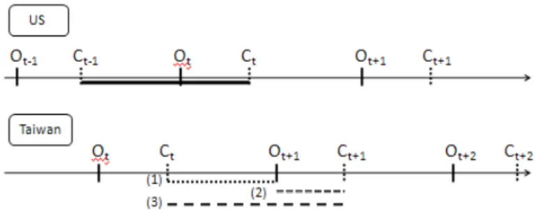
Figure 1: The Trading Periods between US and Taiwan Stock Markets..……...……..…27

Figure 2: The Slope Estimate of the Quantile Regression between S&P 500 and TAIEX,

1995-1997……….……….…...28

1997-2000……….………...29

2000-2007…………...………..………...30

2007-2009……….………...31

1995-2009……….………...32

Figure 7: The Slope Estimate of the Quantile Regression between S&P 500 and OTC,

1995-1997……….………...33

1997-2000………….……….…..34

2000-2007……….……….…..35

2007-2009……….………...36

1995-2009……….………..37

(12)

1997-2000……….………...39

2000-2007……….……….……...40

2007-2009……….……….…...41

1995-2009…….……….…...42

1995-1997……….………..……...43

1997-2000……….…...…...44

2000-2007.……….……..…...45

2007-2009……….……….……...46

1995-2009……..……...………...47

1995-1997……….……….…...48

1997-2000…….………...……...49

2000-2007….………...……...50

(13)

1995-2009………….……….…...52

1995-1997………..…………...53

1997-2000……….…….…...54

2000-2007……….…....55

(14)

1. Introduction

With the decrease in government imposed formal barriers to the flow of capital across

countries, the integration of each country’s capital market has increased over the last several

years. Recent studies examine the interdependence of price change spillover effects across

developed and emerging markets. Eun and Shim (1989) used simulated responses of the

estimated VAR system and found that there is a multi-lateral interaction among national stock

markets. Innovations in the U.S. are quickly transmitted to other markets in a clearly

recognizable fashion.

Moreover, much of the literature shows that US stock market is the important factor

which influences the return of Taiwan stock market. They found that the spillover effect of

stock prices exists from the United States to Taiwan. Wei, Liu, Yang and Chaung (1995)

found that the stock prices of Taiwan stock market are more sensitive than Hong Kong stock

market, although Taiwan is not as open as Hong Kong and Taiwanese dollar is not connected

with the US dollar while the Hong Kong dollar is. Wang and Nguyen (2007) used NYSE,

S&P 500 and NASDAQ to test the transmission between Taiwan and US stocks under

asymmetry. The data period is from 1 January 1997 to 31 October 2001, and they proved that

there is the contagion between Taiwan and US stock markets. Chou, Lin and Wu (1999)

suggested the spillover effects occur for both the mean and the variance of the Taiwan stock

(15)

prices of the US, and the price change spillover effect from the US to Taiwan is significant.

Miyakoshi (2003) used EGARCH and GARCH to investigate the return spillover effects.

However, these previous works mostly used ARCH, GARCH, EGARCH and

M-GARCH models to examine the spillover effects of the stock market. They found the

spillover effects are in the mean and conditional variance, but the mean and conditional

variance could not represent the whole behaviors of these distributions, especially when they

are heterogeneous. In order to concern about the spillover effects of the entire distributions in

different price periods, the paper employs quantile regression model to investigate the price

change spillover effects completely. We also use close-to-open, open-to-close and

close-to-close returns to avoid the sample overlap problems.

The purpose of this study is (1) to examine price change spillover effects across US and

Taiwan stock markets then see if there is any difference when stock price goes up or down,

and (2) to investigate the overreaction effect in open-to-close returns of Taiwan stock market

and detect how the degree in different quantiles.

This paper is organized as follows. In the first part of Section II, we review the literature

related to cross-market spillover effects. In the second part of Section II, we introduce

literature related to overreaction effect. And in the last part of Section II, we also introduce

literature about quantile regression models. Section III introduces the data used in this paper

(16)

(17)

2. Literature Review

2.1 Cross-Market Spillover Effect

Over the past several years, there has been ample research on the price change spillover

effects. Wang, Liao and Shyu (2000) investigated the interactions and the factors of

determining returns and volatility among Asian markets. They found that the return of the

Taiwan stock market is influenced by U.S., Japan, Korea and Singapore. Lee, Rui and Wang

(2004) considered the transmission between the Nasdaq and Asian second board markets,

such as Hong Kong, Japan, South Korea, Singapore and Taiwan. They found that there is

strong evidence of lagged returns and volatility spillover effects from the NASDAQ market to

the Asian second board markets when excluding contemporaneous main board market returns.

Arshanapalli, Doukas and Lang (1995) revealed that there are common stochastic trends in

the US and the Asian stock markets after October 1987 because of a number of stock market

disasters. They also found that the integration degree between Asian stock markets and the US

stock market is higher than it between Asian stock markets and Japan.

Some researches directly examine the price change spillover effects between Taiwan and

the US. Chou, Lin and Wu (1999) used ARCH and M-GARCH to examine the price and

volatility linkages between the US and Taiwan stock market. Spillover effects in price

changes and volatility are found from the US stock market to the Taiwan stock market. Wei,

(18)

price. The result is that the spillover effects should not be observed in the open-to-close

returns under the efficient market hypothesis, since all available information from previous

foreign markets should be fully reflected in opening prices. Moreover, the Taiwanese market

is more sensitive than the Hong Kong market to the price and volatility behaviors of the

advanced markets. We conclude that there are price change spillover effects from the US

(19)

2.2 Overreaction effect

The first research about overreaction effect is raised by J. M. Keynes. He suggested

day-to-day fluctuations in the profits of existing investments have an altogether excessive, and

even an impossible, influence on the markets.

Fama (1970) thought that if the price changes of capital market have no correlation, it’s a

efficient market. He also divided the market into weak-form of the efficient market hypothesis,

semi-strong form of the efficient market hypothesis and strong form of the efficient market

hypothesis.

Roll (1988) looked at the R-squared for regressions of daily and monthly stock returns on

CAPM and APT factors and found that much of the variance in returns can not be explained.

Shiller (1981) revealed that measures of stock price volatility over the past century appear to

be too high to be attributed to new information about future real dividends if there is uncertainty

about future dividends. He concluded that stock prices are too volatile to be explained by

dividend changes and suggested that investors overreact to unobserved stimuli.

Kleidon (1982) found the movement of stock price to be strongly correlated with expected

changes in earnings for the following year and that it is a pattern of overreaction. Investors seem

to overestimate the importance to short-term economic developments.

De Bondt and Thaler (1985) found that investors overreact to short-term (i.e., a few years)

earnings movements. They suggested that most people overreact to the unexpected events, and

the performances of the portfolio of past “losers” are better than past “winners’” under the

overreaction hypothesis. Furthermore, there are large positive returns in losers’ portfolios every

January, and the effect can be observed as long as five years after portfolio formation. Fama and

French (1987) revealed the negative serial correlation in stock returns, and found significant

negative serial correlation in stock returns.

(20)

stock returns that can be attributed to various kinds of news. They found that it is difficult to

explain more than one third of the return variance from macroeconomic news, and concluded

that neither economic variables nor news stories can fully explain extreme aggregate price

movements.

Chan (2003) used monthly stock returns after two sources of stimuli. The first is public

news, which is identifiable from headlines and extreme concurrent monthly returns. The second

is large price movements unaccompanied by any identifiable news. He found that investors seem

to react slowly to valid information, causing drift. Moreover, investors overreact to price shocks,

(21)

2.3 Quantile regression

We usually use regression models to analysis the behavior of explained variables when

the dependent variable is known. In order to explain the model more, there are two ways to

make the error of the model smaller: First, we can use the ordinary least squares method (OLS)

to minimize the error sum of square. Secondly, we can use the least absolute deviations

method (LAD) to minimize the absolute value of error. Quantile regression is the extended

conception of LAD, and it corresponds to fitting the conditional median of the response

variable.

Quantile regression, developed by Koenker and Bassett (1978), is an extension of the

classical least squares estimation of the conditional mean to a collection of models for

different conditional quantile functions (Barnes and Hughes, 2002). By using quantile

regression, we don’t have to make any assumptions to the original distribution, it is

nonparametric. It is useful to analysis the data when the conditional distribution does not have

a normal distribution or standard shape, such as an asymmetric or fat-tailed distribution.

Koenker and Bassett (1982) suggest that given the regression parameter, if we don’t change

the plus and minus signs of the residual, the estimate won’t change even the distance between

sample and quantile is changed. In other words, no matter the outlier is large or small,

quantile regression is robustness.

(22)

can be supposed as follows:

+ = t

β

t x

y ' e t, t=1,...,Τ. (1)

Given the data

(

y ,_t x_t′

)

′ for t=1,...,Τ , where x is _t k×1, β includes regression coefficient of each variable, and e is error term. t

Quantile regression which is suggested by Koenker and Bassett(1982) extends the

concept to calculate the quantile:

(

)

      ′ − − + ′ − =

_∑

′ ≥ < ′ ∧ β β θ

θ

β

θ

β

t t x t t y y x t t t t x y x y 1 min arg , (2)

where θ is the quantile, and 0 <θ < 1. When θ is 0.5, (2) equation can be written in

∑

Τ = ∧ ′ − = _t ₁ yt xtβ

βθ , and it is exactly the objective function for LAD estimation.

The θth quantile regression estimator of βcan be obtained by minimizing the weighted

average of the absolute value of error:

( )

(

)

      ′ − − + ′ − Τ =

_∑

′ ≥ β

β

θ

< ′β

β

θ

β

t t x t t y t ty x t t t t t y x y x V : : 1 1 ; , (3)

if θ is smaller (bigger) than 0.5, the positive error of weight of function is smaller (bigger), and the negative error of weight is bigger (smaller). So it is the left of the distribution. When

θ is 0.5, we can two times (3):

( )

(

)

∑

Τ = Τ Τ = = _Τ − ′ 1 1 5 . 0 ; 2 t t t m x y V V β β β , so we can say a

regression estimated via the method of LAD which is referred as a “median regression is a

(23)

In order to minimize (3), the first order condition of (3) is as follows:

(

)

∑

Τ = ′ − Τ 1 1 t t t x y β ϕθ

∑

(

{ }

)

Τ = − ′ < = − Τ = 1 0 0 1 1 t x y t _t _t x θ _β , (4) we can obtain the

θ

th quantile regression estimator of β (βθ

∧

) by solving (4).

Because we can’t find out the closed form solution of (4), we have to find another way to

solve the equation.

Nonlinear optimization, the traditional method of solution, can’t be used to solve the

equation. Koenker and Machado (1999) suggest the equation (4) is also the quasi-maximum

likelihood estimator which is used asymmetric Laplace (double exponential) density:

{

( )

}

exp ) 1 ( ) ; (e e f θ =θ −θ ρ_θ

(24)

3. Data

3.1 Sample

In this section, we examine daily stock prices of Taiwan and the United State from 7

November 1995 to 26 March 2009. In the case of the Taiwan stock market, we use the Taiwan

Weighted Stock Index and Over-the-Counter index. For the United States we use S&P500.

Because of different closing hours, we delete the data which only has partial market

information. There are 3178 daily returns included finally.

We retrieve the raw data of the Taiwan Weighted Stock Index and Over-the-Counter

index for the entire period from TEJ, and S&P500 from Yahoo Finance

(www.yahoo.com/finance).

In this paper, we use close-to-close returns of US to investigate whether the former

returns of US effects the returns of Taiwan. We discuss three market segments of Taiwan

stock which comprise close-to-open, open-to-close and close-to-close returns respectively.

We wanted to discuss the influences of different periods, especially between the Asian

Financial Crisis in 1997and recent Financial Tsunami recently, so we considered four periods

as follows: The first period is before the Asian Financial Crisis, because Over-the-Counter

index of TEJ starts from November 1995, we choose the data from 7 November1995 to 30

June 1997. According to Cheung, Cheung and Ng (2007) and Chang, M. C. (2008), the

(25)

Tsunami starts from the bankruptcy of New Century Financial Corporation in March 2007 by

some research (Ashcraft and Schuermann, 2008) and the international financial news of

Yahoo. The third period is between the crisis and Financial Tsunami from 3 July 2000 to 27

February 2007. The last period is during the tsunami from 1 March 2007 to 26 March 2009.

We use the following picture to understand the trading periods between US and Taiwan

easily. The “Ot” represents the opening stock price of t day, and the “Ct” represents the closing

stock price of t day. Because the trading dates of US are later than Taiwan’s, we can say that t

day of Taiwan stock market is influenced by t-1 day of US stock market. For example, the

return of US’s t day (the period from Ct-1 to Ct)affects three periods of Taiwan stock market:

(1).The period from the closing price of t day to the opening price of t+1 day (from Ct to Ot+1.)

(2). The period from the opening price of t+1 day to the closing price of t+1 day (from Ot+1 to

Ct+1.) (3).The period from the closing price of t day to the closing price of t+1 day (from Ct to

Ct+1,) and so on.

(26)

3.2 Descriptive Statistics

In Table 1, we show the descriptive statistics of the returns of Taiwan and US stock

markets from 1995/11/7 to 2009/3/26. Panel A shows the descriptive statistics for the

close-to-open returns of Taiwan stock markets and close-to-close returns of US stock markets.

The daily close-to-open returns are calculated by 100×log (Ρ_tOpen/Ρ_tClose₋₁ ).

＜Panel A is inserted about here＞

Panel B shows the descriptive statistics for the open-to-close returns of Taiwan stock

markets and close-to-close returns of US stock markets. The daily open-to-close returns are

calculated by 100×log (Ρ_tClose/Ρ_tOpen).

＜Panel B is inserted about here＞

Panel C shows the descriptive statistics for the close-to-close returns of Taiwan stock

markets and close-to-close returns of US stock markets. The daily close-to-close returns are

calculated by 100×log (Ρ_tClose/Ρ_tClose₋₁ ). And all the descriptive statistics of the returns of the series are given in Table1.

＜Panel C is inserted about here＞

In Table 1, we can know the difference between close-to-open, open-to-close and

close-to-close returns of TAIEX and OTC over the sample period from 1995/11/7 to

2009/3/26. The means of close-to-open returns of TAIEX and OTC are positive (Panel 1),

(27)

close-to-close returns of TAIEX is positive, however, OTC’s is negative (Panel 3).

For volatility, it is shown that the standard deviation of TAIEX and OTC are the smallest

in close-to-open returns. And the standard deviation of TAIEX and OTC are the highest in

close-to-close returns.

Close-to-open and close-to-close returns of TAIEX and OTC are negatively skewed, so

we know they shift to the left. And open-to-close returns of TAIEX and OTC are positively

skewed, so we know they shift to the right. Moreover, all moments of the returns have excess

kurtosis.

The means of close-to-close returns of NASDAQ, Dow Jones and S&P 500 are positive

and have excess kurtosis. Dow Jones and S&P 500 are negatively skewed and shift to the left.

However, NASDAQ is positive and shifts to the right.

In Panel 1, it is indicated that the volatility of NASDAQ return is the highest and the

close-to-open return of TAIEX is the smallest. In Panel 2, the volatility of NASDAQ return is

the highest and the Dow Jones is the smallest. And it is shown that the volatility of OTC

return is the highest and the Dow Jones is the smallest in Panel 3.

All the variables we use are returns, so we will not have any spurious regression. We can

use quantile regression directly.

(28)

4. Estimation Results

We regard S&P 500 as the independent variable, TAIEX and OTC as the dependent

variables. We use E-VIEWS to consider the quantile regression between the returns of S&P

500 and the returns of TAIEX and OTC respectively. Every 0.05 quantile from 0.05 to 0.95

(left to right) for each sample was chosen. Moreover, 0.01 and 0.99 quantiles are chosen,

because we want to know the highest and the lowest stock prices. The interception and slope

estimates are under 95% confidence interval and there are 21 results of quantile regression in

each sample period.

Table 2 to Table 11 document the empirical results of the influences from the returns of

US stock market to the returns of close-to-open stock market of Taiwan over the sample

period from 1995 to 2009.

Table 2 presents the results from 1995/11/7 to 1997/6/30, and most of the coefficients of

slope are significant positive at 5% or 10% significant level, except for θ= 0.05, 0.55, 0.6, 0.75, 0.8, 0.9. Moreover, it becomes non significant negative correlation where θ= 0.01. After 1997/7/2 (Table 3 to Table 5), there are significant positive correlations at 5%

significance level. And Table 6 shows that there is significant positive correlation between the

returns of US stock market and the close-to-open returns of TAIEX at 5% significance level

from 1995 to 2009.

(29)

< Table 3 is inserted about here >

Table 7 to Table 11 present the correlations between US stock market and the

close-to-open returns of OTC from1995/11/7 to 2009/3/26. In Table 7, there is non significant

positive correlation except for θ= 0.05, 0.9, 0.95 at 5% significance level and θ= 0.35 at 10% significance level. After 1997/7/2 (Table 8 to Table 10), there are significant positive

correlations at 5% significance level. Table 11 shows that there is significant positive

correlation between the returns of US stock market and the close-to-open returns of OTC at

5% significance level from 1995 to 2009.

Table 12 to Table 21 document the empirical results of the influences from the returns of

US stock market to the returns of open-to-close stock market of Taiwan over the sample

(30)

negative. Moreover, we find that there are significant negative at θ= 0.05 at 5% significance level, and at θ= 0.15, 0.85, 0.9, 0.95, 0.99 at 10% significance level. We know that there are negative correlations between the returns of US stock market and the returns of open-to-close

stock market of TAIEX from 1995/11/7 to 1997/6/30, though significant negative correlations

only occurred at the highest or lowest price.

Table 13 shows all of the coefficients of slope are significantly negative. Moreover, we

find that half of the quantiles are significant negative correlations. When θ= 0.01, 0.05, 0.1, 0.25, 0.8, 0.85, there are significant negative correlations at 5% significance level, and there

are significant negative correlations at θ= 0.15, 0.35, 0.75 at 10% significance level. < Table 13 is inserted about here >

After 2000/7/3, almost all the coefficients of slope are significant negative, except for

θ= 0.99 from 2000/07/03-2007/02/27 and θ= 0.05, 0.1, 0.15 from 2007/3/1 to 2009/3/26. There seems to be a significant negative trend when time goes by. Table 16 shows that there is

significant negative correlation between the returns of US stock market and the open-to-close

returns of TAIEX at 5% significance level from 1995 to 2009.

(31)

Table 17 shows that all the coefficients of slope are negative, and we find that there are

significant negative at θ= 0.01, 0.05 at 5% significance level, and at Q= 0.45, 0.9, 0.95 at 10% significance level. In Table 18, Table 19 and Table 20, almost all the coefficients of slope

are significant negative at 5% significance level, except for θ= 0.2, there is non significant at 10% level of significance from 1997/7/2 to 2000/6/30 (Table 18), and there is non significant

at θ= 0.1 at 10% level of significance from 2007/03/01-2009/03/26 (Table 20). Table 21 shows that there is significant negative correlation between the returns of US stock market

and the open-to-close returns of OTC at 5% significance level from 1995 to 2009.

Table 22 to Table 31 are documented the empirical results of the influences from the

returns of US stock market to the returns of close-to-close stock market of Taiwan over the

sample period from 1995 to 2009. Table 22 shows that most of the coefficients of slope are

non significant positive correlations, however, the coefficients of slope are non significant

negative correlations when θ= 0.1, 0.01, 0.8, 0.85, 0.9, 0.95. There is significant negative correlation at θ= 0.01 at 5% significance level, but there is significant positive correlation at

(32)

θ= 0.99 at 10% significance level. After 1997/7/2 (Table 23, Table 24 and Table 25), there are almost significant positive correlations between the returns of US stock market and the

returns of TAIEX at 5% or 10 % significance level, except for θ= 0.95, 0.99 from 1997/7/2 to 2000/6/30 (Table 23) is non significant at 10% level of significance. Table 26 shows that

there is significant positive correlation between the returns of US stock market and the

close-to-close returns of TAIEX at 5% significance level from 1995 to 2009.

In Table 27, most of the coefficients of slope are non significant positive correlations

between the returns of S&P 500 and the close-to-close returns of OTC from 1995/11/06 to

1997/06/30, except when θ= 0.01, 0.05, 0.35, 0.6, 0.8, 0.9, 0.95, there are non significant negative effects. Furthermore, there is significant negative correlation at θ= 0.01 at 5% significance level. After 1997/7/2, there is significant positive correlation at 5% significance

level, except for θ = 0.95 and 0.99, there are non significant positive effects at 10% significance level. Table 31 shows that there is significant positive correlation between the

(33)

from 1995 to 2009.

We analyze how US stock mark influences Taiwan stock market at different quantiles by

using the quantile regression. And it can give us the suggestion what we should react as the

price goes up or down. This paper not only confirms the prior studies that Taiwan stock

market is influenced by the stock price of the US, but also discovers the overreaction effect.

We summarize the results in Table 32, 33, 34, 35, 36, 37, 38, 39, 40 and our findings are as

follows:

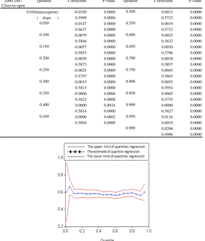
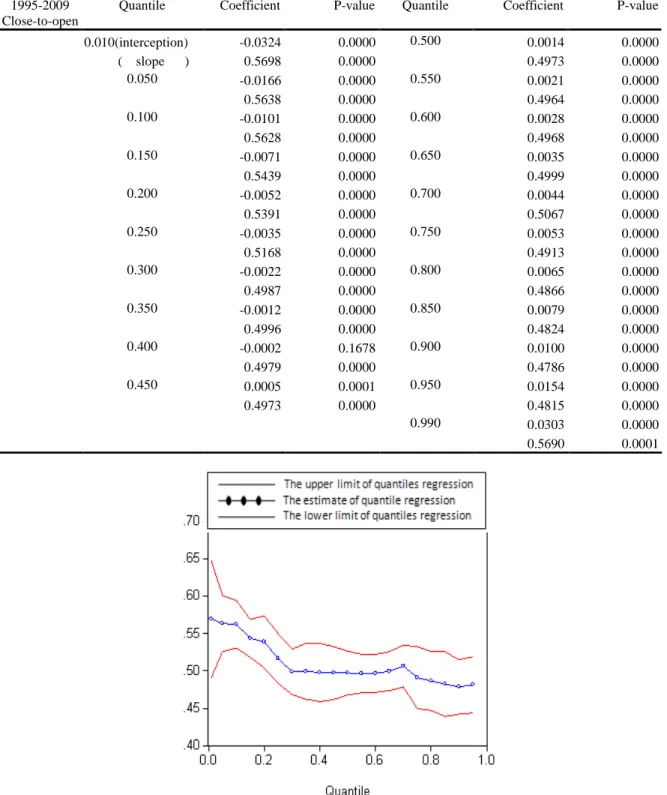
1. For the close-to-open returns, there is significant positive effect from US to Taiwan stock

markets from 1995/11/7 to 2009/3/26. However, the price change spillover effect exists

when the stock price goes up or down greatly from 1995/11/7 to 1997/6/30 (Table 32 and

33). There seems to be a significant positive trend not only in TAIEX but also in OTC as

time goes by. In other words, we can say that there is the spillover effect from US stock

market to the close-to-open return of Taiwan stock market. Table 35 reports the slope

(34)

2009. We can know that both of the slope estimates are positive. In other words, there are

positive correlations not only between S&P 500 and close-to-open returns of TAIEX, but

also between S&P 500 and close-to-open returns of OTC. Moreover, we can find that the

slope estimates are different in most of the quantiles. OLS might underestimate the slope

estimate when price goes down but overestimate it when price goes up.

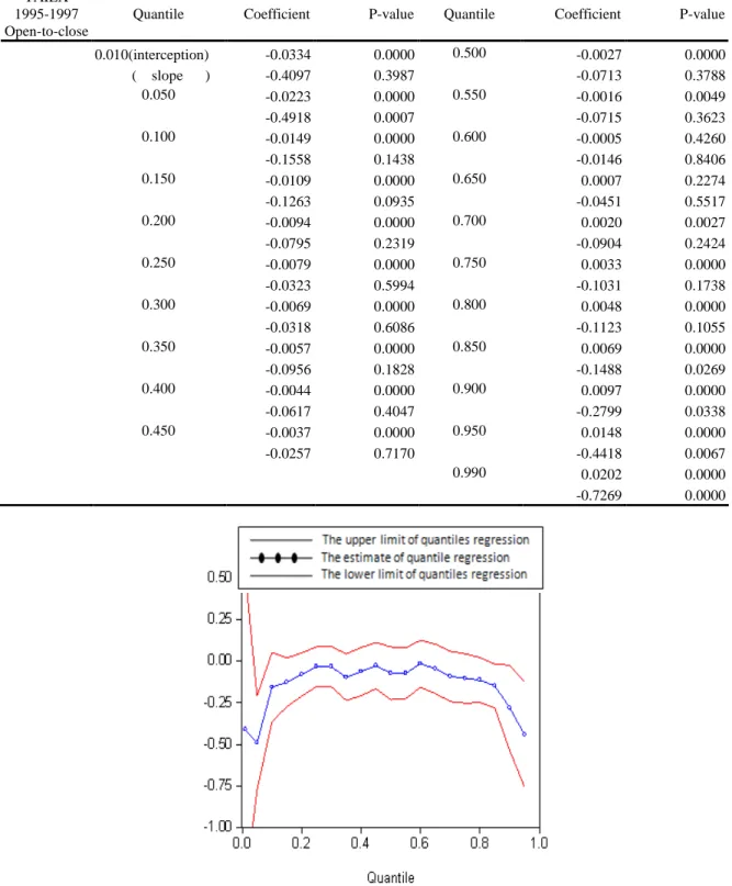
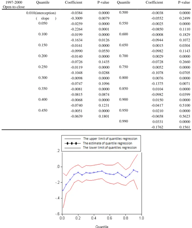
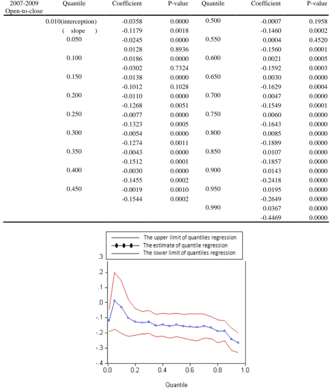
2. For the open-to-close returns, there is significant negative correlation between US and

Taiwan stock markets from 1995/11/7 to 2009/3/26. In other words, there are

overreaction effects both in TAIEX and OTC. For TAIEX, the negative effect is stronger

when the stock price goes up greatly from 1995/11/7 to 1997/6/30, however, the negative

effect is stronger when the stock price goes down greatly from 1997/7/2 to 2000/6/30.

From 2000/7/3 to 2009/3/26, the negative effect is significant. For OTC, the negative

impact is stronger when the stock price goes up or down greatly from 1995/11/7 to

2000/6/30. From 2000/7/3 to 2009/3/26, the negative effect is significant. Table 37

reports the slope estimate of both the quantile regression and ordinary least squares

method from 1995 to 2009. We can know that both of the slope estimates are negative. In

other words, there are negative correlations not only between S&P 500 and open-to-close

returns of TAIEX, but also between S&P 500 and open-to-close returns of OTC.

Moreover, we can find that the slope estimates are different in most of the quantiles. OLS

(35)

OLS underestimates the slope estimates.

3. For the close-to-close returns, there is significant positive correlation between US and

Taiwan stock markets from 1995/11/7 to 2009/3/26, except for the returns from

1995/11/7 to 1997/6/30. There is a negative effect from U.S. to Taiwan when the stock

price goes down greatly from 1995/11/7 to 1997/6/30. Furthermore, there seems to be a

significant positive trend not only in TAIEX but also in OTC as time goes by. And we can

conclude there is the spillover effect from US stock market to the close-to-close return of

Taiwan stock market. Table 40 reports the slope estimate of both the quantile regression

and ordinary least squares method from 1995 to 2009. We can know that both of the slope

estimates are positive. In other words, there are positive correlations not only between

S&P 500 and close-to-close returns of TAIEX, but also between S&P 500 and

close-to-close returns of OTC. Moreover, we can find that the slope estimates are

different in most of the quantiles. OLS might underestimate the slope estimate when price

goes down greatly, but otherwise overestimates the slope estimates.

(36)

(37)

5. Conclusion

In this paper, we use quantile regression and learn that both spillover effects and

overreaction effect exist from US stock market to Taiwan stock market, and we separate time

period from 1995/11/7 to 1997/6/30, 1997/6/30 to 2000/6/30, 2000/7/3 to 2007/2/27, and

from 2007/3/1 to 2009/3/26 to know the spillover effects and overreaction effect respectively.

We not only demonstrate the past research that there are spillover effects in close-to-open and

close-to-close returns (Chou, Lin, Wu, 1999 and Chang, 2008), but also find that there is a

overreaction effect in open-to-close returns. Furthermore, both of spillover effects and

overreaction effect become stronger over time.

We find that if we use OLS, we can only know there is positive or negative correlation

between U.S. and Taiwan on average. And OLS overestimates or underestimates the slope

estimate at different quantiles. Quantile regression makes us know the whole behavior of the

distribution, no matter the stock price goes up or down.

Because the spillover and overreaction effects exist from US stock market to Taiwan

stock market, there are some suggestions for investors. Firstly, because of the spillover effects,

we can judge whether tomorrow’s opening price or closing price of Taiwan stock market will

goes up by today’s closing price of US. Secondly, because of the overreaction effect, if the

closing stock price of US goes down and the opening stock price of Taiwan goes down greatly,

(38)

during Financial Tsunami. So investors should be more cautious as TAIEX stock prices go

down during Financial Tsunami.

In this paper, we didn’t take the limit regulation of stock price into consideration. The

price limit regulation delays stock price discovery process if the limits are hit (Wang, L. H.,

2000), so it could be a factor that influences overreaction from US to Taiwan. After 1989, the

price limit regulation changes from 5% to 7%, and there are seven times that the down limits

adjust to 3.5% in our time period. The seven times are as follows:

1. 1999/9/27~1999/10/9: 921 earth quake.

2. 2000/3/20~2000/3/24: the turnover of the regime.

3. 2000/10/4~2000/10/11: the resignation of Premier.

4. 2000/10/20~2000/11/7: the discontinuity of the fourth nuclear power plant.

5. 2000/11/21~2000/12/31: the falling of Taiwan stock market by 320 points.

6. 2001/9/19~2001/9/21: September 11 attacks.

7. 2008/10/13~2008/10/17: financial tsunami. Because each time period of these is short, we

didn’t take into account in this paper, the following researchers can expand in this

(39)

Reference

Ashcraft, A. B. and Schuermann, T., 2008. Understanding the securitization of subprime mortgage credit. Federal Reserve Bank of New YorkStaff Reports.

Arshanapalli, B., Doukas, J. and Lang, L. H. P., 1995. Pre and post-October 1987 stock market linkages between US and Asian markets. Pacific-Basin finance journal 3, 57-73.

Ghosh, A., Saidi, R. and Johnson, K. H., 1999. Who moves the Asia-Pacific stock markets-US or Japan? Empirical evidence based on the theory of cointegration. The Financial Review 34, 159-170.

Lin, B. H. and Yeh, S. K., 2000. On the distribution and conditional heteroscedasticity in Taiwan stock prices. Journal of Multinational Financial Management, 10, 367-395.

Lee, B. S., Rui, O. M., Wang, S. S. and Shatin, 2001. Information transmission between NASDAQ and Asian second board markets. Journal of banking and finance, Vol. 28, N. 7, 2004, 1637-1670. Chang, M. C., 2008. The dynamic linkage of Taiwan and US stock markets. Wang, Working Paper

(National Chiao Tung University).

Cheung, Y. L., Cheung, Y. W., Ng C. C., 2007. East Asian equity markets, financial crises, and the Japanese currency. Journal of the Japanese and International Economics 21, 138-152.

Cutler, D. M., Poterba, J. M., Summers, L. H., 1989. What moves stock prices? Journal of Portfolio

Management 15, 4–12.

Kahneman, D. and Tversky, A., 1982. Intuitive prediction: Biases and corrective procedures. In D. Kahneman, P. Slovic, and A. Tversky, (eds.), Judgment Under Uncertainty: Heuristics and Biases. London: Cambridge University Press.

Eugene F. Fama and Kenneth R. French, 1987. Commodity futures prices: Some evidence on forecast power, premiums, and the theory of storage. Journal of Business, vol. 60, no. 1, 55-73.

Eun, C. and Shim, S.,1989, International transmission of stock market movements. Journal of

(40)

Fama, E. F., 1970. Efficient capital markets–A review of theory and empirical work. Journal of

Finance, vol. 25, Issue 2, 383-417.

French, K.R., Roll, R.W., 1986. Stock return variance: the arrival of information and the reaction of traders. Journal of Financial Economics 19, 3–30.

G. De. Santis and Imrohoroglu, S., 1997. Stock returns and volatility in emerging financial markets.

Journal of International Money and Finance, Vo. 16, No. 4, 561-579.

J. M. Keynes,1964. The general theory of employment, interest and money. London: Harcourt Brace

Jovanovich.

K. C. John Wei, Y. J. Liu, C. C. Yang and Chaung, G. S., 1995. Volatility and price change spillover effects across the developed and emerging markets. Pacific-Basin Finance Journal 3, 113-136.

Kleidon Allan, 1982. Stock prices as rational forecasters of future cash flows. Dept. of Accounting and Finance, Monash University.

Koenker, R. and Bassett G.W., 1982, Robust tests for heteroscedasticity based on regression quantiles.

Journal of Derivatives, 3, 73-84.

Wang, Kuan-Min and Thanh-Binh Nguyen Thi, 2007. Testing for contagion under asymmetric dynamics: Evidence from the stock markets between US and Taiwan. Physica A 376, 422–432.

Lee, B. S., Rui, O. M. and Wang, S. S., 2004. Information transmission between the NASDAQ and Asian second board markets. Journal of Banking and Finance 28, 1637-1670.

Wang, L. H., 2000. A systematic risk and liquidity analysis of price limits mechanism on textiles and electronics in Taiwan. Working Paper (National Chiao Tung University).

Veronesi, P., 1999. Stock market overreaction to bad news in good times: A rational expectations equilibrium model. The Review of Financial Studies Vol. 12, No.5, 975–1007.

Chou, R.Y., Lin, Jin-Lung and Wu, Chung-Shu, 1999. Modeling the Taiwan stock market and international linkages. Pacific Economic Review, 4: 3, 305-320.

Koenker, R. and G. Bassett Jr., 1978. Regression quantiles. Econometrica, Vol. 46, No. 1., pp. 33-50.

(41)

Economics 12, 371–386.

Roll, R.W., 1988. On computing mean returns and the small firm premium. Journal of Finance 43, 541–566.

Shiller, R.J., 1981. Do stock prices move too much to be justified by subsequent changes in dividends?

American Economic Review 71, 421–498.

Miyakoshi, T., 2003. Spillovers of stock return volatility to Asian equity markets from Japan and the US. Journal of International Financial Markets, Institutions & Money 13, 383-399.

Wang, Y. M., Liao, S. L. and Shyu, S., 2000. The relationships among Asian stock markets- The test of dynamic process. Asia Pacific Management Review 5, 15-27. (In Chinese)

Chan, W. S., 2003. Stock price reaction to news and no-news: drift and reversal after headlines.

Journal of Financial Economics 70, 223–260.

Thaler, R. H., 1985. Does the stock market overreaction? Journal of Finance, 793-805

Werner F. M. De Bondt and Richard H. Thaler, 1987. Further evidence on investor overreaction and stock market seasonality. The Journal of Finance * Vol. Xlii, No.3.

Y. Hamao, R. W. Masulis and V. Ng, 1990. Correlations in price changes and volatility across international stock markets. The Review of Financial Studies, Vol. 3, No. 2, 281-307.

(42)

TABLE 1 Descriptive Statistics

Panel A : Descriptive Statistics for Taiwan and US Stock Markets’ Returns and ADF

Unit Root Test,

1995/11/7 to

2009/3/26

Panel B : Descriptive Statistics for Taiwan and US Stock Markets’ Returns and ADF Unit Root Test, 1995/11/7 to 2009/3/26

Panel C : Descriptive Statistics for Taiwan and US Stock Markets’ Returns and ADF Unit Root Test, 1995/11/7 to 2009/3/26

Close-to-open Close-to-close

TSE OTC S&P 500

Mean 0.001839 0.000692 0.000101 Median 0.002634 0.001556 0.000615 Maximum 0.081902 0.079184 0.102457 Minimum -0.155686 -0.162348 -0.094695 Std. Dev. 0.011864 0.013015 0.013371 Skewness -1.193241 -0.892372 -0.133385 Kurtosis 18.76169 15.14800 10.23191 Observations 3178 3178 3178 Open-to-close Close-to-close

TSE OTC S&P 500

Mean -0.001806 -0.000757 0.000101 Median -0.001873 -0.001043 0.000615 Maximum 0.067319 0.079807 0.102457 Minimum -0.074804 -0.079415 -0.094695 Std. Dev. 0.013219 0.015338 0.013371 Skewness 0.083763 0.246014 -0.133385 Kurtosis 5.275018 5.034203 10.23191 Observations 3178 3178 3178 Close-to-close Close-to-close

TSE OTC S&P 500

Mean 3.22E-05 -6.48E-05 0.000101

Median 1.76E-05 -0.000109 0.000615 Maximum 0.085198 0.097454 0.102457 Minimum -0.126043 -0.140420 -0.094695 Std. Dev. 0.016723 0.019004 0.013371 Skewness -0.247889 -0.080337 -0.133385 Kurtosis 6.323649 5.694679 10.23191 Observations 3178 3178 3178

(43)

TABLE 2

Quantile Regression, 1995/11/07-1997/06/30

Independent Variable: The Returns of Close-to-close Stock Price of S&P 500 Dependent Variable: The Returns of Close-to-open Stock Price of TAIEX

Figure 2: The slope estimate of the quantile regression between S&P 500 and TAIEX under 95% confidence interval.

TAIEX 1995-1997 Close-to-open

Quantile

Coefficient P-value Quantile Coefficient P-value

0.010(interception) -0.0170 0.0000 0.500 0.0048 0.0000 ( slope ) -0.1359 0.3265 0.0954 0.0808 0.050 -0.0096 0.0000 0.550 0.0055 0.0000 0.0928 0.2255 0.0868 0.1132 0.100 -0.0051 0.0000 0.600 0.0060 0.0000 0.2102 0.0009 0.0924 0.1045 0.150 -0.0028 0.0000 0.650 0.0068 0.0000 0.2694 0.0000 0.1103 0.0837 0.200 -0.0007 0.2416 0.700 0.0073 0.0000 0.2227 0.0000 0.1305 0.0558 0.250 0.0007 0.1775 0.750 0.0080 0.0000 0.1716 0.0023 0.1045 0.1528 0.300 0.0015 0.0038 0.800 0.0089 0.0000 0.1652 0.0043 0.0734 0.3317 0.350 0.0023 0.0000 0.850 0.0107 0.0000 0.1590 0.0058 0.1386 0.0790 0.400 0.0034 0.0000 0.900 0.0123 0.0000 0.1205 0.0249 0.1182 0.1205 0.450 0.0042 0.0000 0.950 0.0178 0.0000 0.0934 0.0802 0.3763 0.0623 0.990 0.0261 0.0000 0.5785 0.0000

(44)

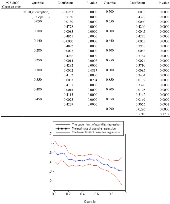
TABLE 3

Figure 3: The slope estimate of the quantile regression between S&P 500 and TAIEX under 95% confidence interval.

Quantile Coefficient P-value Quantile Coefficient P-value

0.010(interception) -0.0267 0.0000 0.500 0.0033 0.0000 ( slope ) 0.5180 0.0000 0.4322 0.0000 0.050 -0.0130 0.0000 0.550 0.0040 0.0000 0.4778 0.0000 0.4206 0.0000 0.100 -0.0083 0.0000 0.600 0.0045 0.0000 0.4961 0.0000 0.4223 0.0000 0.150 -0.0050 0.0000 0.650 0.0055 0.0000 0.4872 0.0000 0.3953 0.0000 0.200 -0.0027 0.0000 0.700 0.0063 0.0000 0.4266 0.0000 0.3764 0.0000 0.250 -0.0014 0.0007 0.750 0.0074 0.0000 0.4292 0.0000 0.3710 0.0000 0.300 -0.0002 0.4817 0.800 0.0085 0.0000 0.4102 0.0000 0.3434 0.0000 0.350 0.0007 0.0294 0.850 0.0102 0.0000 0.4191 0.0000 0.3378 0.0000 0.400 0.0015 0.0000 0.900 0.0125 0.0000 0.4115 0.0000 0.3142 0.0000 0.450 0.0023 0.0000 0.950 0.0169 0.0000 0.4239 0.0000 0.3055 0.0001 0.990 0.0286 0.0000 0.5718 0.1739

(45)

TABLE 4

0.010(interception) -0.0270 0.0000 0.500 0.0016 0.0000 ( slope ) 0.4987 0.0000 0.5728 0.0000 0.050 -0.0111 0.0000 0.550 0.0021 0.0000 0.5772 0.0000 0.5623 0.0000 0.100 -0.0060 0.0000 0.600 0.0027 0.0000 0.5706 0.0000 0.5561 0.0000 0.150 -0.0041 0.0000 0.650 0.0034 0.0000 0.6010 0.0000 0.5537 0.0000 0.200 -0.0027 0.0000 0.700 0.0040 0.0000 0.6065 0.0000 0.5513 0.0000 0.250 -0.0017 0.0000 0.750 0.0047 0.0000 0.5857 0.0000 0.5591 0.0000 0.300 -0.0009 0.0000 0.800 0.0055 0.0000 0.5771 0.0000 0.5545 0.0000 0.350 -0.0002 0.1977 0.850 0.0067 0.0000 0.5705 0.0000 0.5677 0.0000 0.400 0.0005 0.0028 0.900 0.0085 0.0000 0.5615 0.0000 0.5779 0.0000 0.450 0.0011 0.0000 0.950 0.0122 0.0000 0.5709 0.0000 0.5584 0.0000 0.990 0.0215 0.0000 0.5902 0.0000

(46)

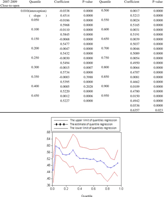
TABLE 5

0.010(interception) -0.0338 0.0000 0.500 0.0017 0.0000 ( slope ) 0.4514 0.0000 0.5213 0.0000 0.050 -0.0186 0.0000 0.550 0.0024 0.0000 0.5968 0.0000 0.5165 0.0000 0.100 -0.0110 0.0000 0.600 0.0031 0.0000 0.5845 0.0000 0.5191 0.0000 0.150 -0.0068 0.0000 0.650 0.0039 0.0000 0.5477 0.0000 0.5037 0.0000 0.200 -0.0047 0.0000 0.700 0.0046 0.0000 0.5432 0.0000 0.5089 0.0000 0.250 -0.0030 0.0000 0.750 0.0054 0.0000 0.5494 0.0000 0.4950 0.0000 0.300 -0.0015 0.0007 0.800 0.0064 0.0000 0.5734 0.0000 0.4707 0.0000 0.350 -0.0003 0.3988 0.850 0.0081 0.0000 0.5395 0.0000 0.4662 0.0000 0.400 0.0005 0.2028 0.900 0.0109 0.0000 0.5220 0.0000 0.4780 0.0000 0.450 0.0012 0.0006 0.950 0.0150 0.0000 0.5227 0.0000 0.4942 0.0000 0.0336 0.0000 0.6357 0.023

(47)

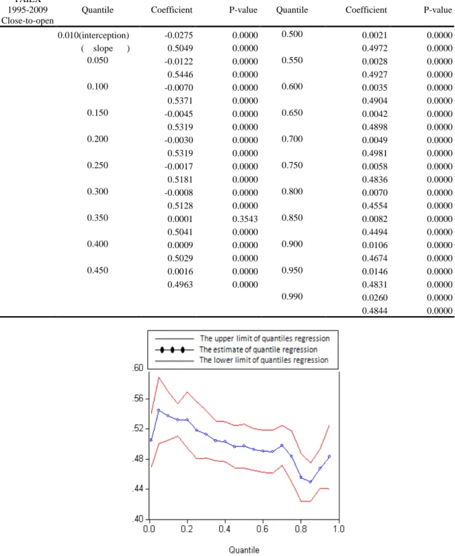
TABLE 6

(48)

TABLE 7

Independent Variable: The Returns of Close-to-close Stock Price of S&P 500 Dependent Variable: The Returns of Close-to-open Stock Price of OTC

Figure 7: The slope estimate of the quantile regression between S&P 500 and OTC under 95% confidence interval.

OTC

1995-1997 Close-to-open

0.010(interception) -0.0267 0.1702 0.500 0.0004 0.2025 ( slope ) 0.1296 0.9891 0.0428 0.2876 0.050 -0.0117 0.0000 0.550 0.0013 0.0002 0.2380 0.0038 0.0737 0.1063 0.100 -0.0069 0.0000 0.600 0.0022 0.0000 0.0499 0.5338 0.0661 0.2235 0.150 -0.0041 0.0000 0.650 0.0030 0.0000 0.0663 0.2924 0.0960 0.1605 0.200 -0.0026 0.0000 0.700 0.0044 0.0000 0.0559 0.1378 0.1133 0.1729 0.250 -0.0020 0.0000 0.750 0.0060 0.0000 0.0569 0.1055 0.0754 0.4628 0.300 -0.0010 0.0005 0.800 0.0075 0.0000 0.0710 0.0370 0.1800 0.2481 0.350 -0.0005 0.0772 0.850 0.0107 0.0000 0.0601 0.0940 0.1628 0.1190 0.400 -0.0003 0.4126 0.900 0.0132 0.0000 0.0585 0.1194 0.2628 0.0236 0.450 0.0000 0.8901 0.950 0.0190 0.0000 0.0360 0.3635 0.3675 0.0301 0.990 0.0383 0.0000 0.6022 0.2791

(49)

TABLE 8

OTC 1997-2000 Close-to-open

0.010(interception) -0.0335 0.0000 0.500 0.0000 0.9375 ( slope ) 0.4777 0.0000 0.4777 0.0000 0.050 -0.0192 0.0000 0.550 0.0015 0.0005 0.6085 0.0000 0.4851 0.0000 0.100 -0.0128 0.0000 0.600 0.0025 0.0000 0.6072 0.0000 0.4846 0.0000 0.150 -0.0103 0.0000 0.650 0.0036 0.0000 0.5945 0.0000 0.4965 0.0000 0.200 -0.0080 0.0000 0.700 0.0048 0.0000 0.5658 0.0000 0.5026 0.0000 0.250 -0.0064 0.0000 0.750 0.0062 0.0000 0.5556 0.0000 0.4669 0.0000 0.300 -0.0048 0.0000 0.800 0.00787 0.0000 0.5233 0.0000 0.4673 0.0000 0.350 -0.0036 0.0000 0.850 0.0101 0.0000 0.5133 0.0000 0.4704 0.0000 0.400 -0.0020 0.0000 0.900 0.0138 0.0000 0.4770 0.0000 0.4601 0.0000 0.450 -0.0009 0.0510 0.950 0.0199 0.0000 0.4573 0.0000 0.4191 0.0033 0.990 0.0352 0.0002 0.3104 0.5940

(50)

TABLE 9

0.010(interception) -0.0350 0.0000 0.500 0.0013 0.0000 ( slope ) 0.5999 0.0006 0.5723 0.0000 0.050 -0.0147 0.0000 0.550 0.0019 0.0000 0.6637 0.0000 0.5723 0.0000 0.100 -0.0079 0.0000 0.600 0.0025 0.0000 0.5846 0.0000 0.5632 0.0000 0.150 -0.0057 0.0000 0.650 0.0030 0.0000 0.5853 0.0000 0.5706 0.0000 0.200 -0.0039 0.0000 0.700 0.0038 0.0000 0.5873 0.0000 0.5857 0.0000 0.250 -0.0025 0.0000 0.750 0.0045 0.0000 0.5797 0.0000 0.5865 0.0000 0.300 -0.0015 0.0000 0.800 0.0055 0.0000 0.5815 0.0000 0.5954 0.0000 0.350 -0.0006 0.0006 0.850 0.0065 0.0000 0.5823 0.0000 0.5755 0.0000 0.400 0.0000 0.8924 0.900 0.0080 0.0000 0.5814 0.0000 0.5627 0.0000 0.450 0.0006 0.0002 0.950 0.0116 0.0000 0.5694 0.0000 0.6019 0.0000 0.990 0.0206 0.0000 0.4986 0.0000

(51)

TABLE 10

美國對台灣股市外溢效果之分量迴歸分析

國

立

交

通

大

學

經營管理研究所

碩

士

論

文

美國對台灣股市外溢效果之分量迴歸分析

Quantile Regression Analysis of the Spillover Effect of

US-Taiwan Stock Markets

研 究 生：蔡佳樺

指導教授：周雨田 教授

中

中

中

中 華

華

華

華 民

民

民

民 國

國

國

國 九十八

九十八 年

九十八

九十八

年

年

年 六

六

六

六 月

月

月

月

美國對台灣股市外溢效果的分量回歸分析

美國對台灣股市外溢效果的分量回歸分析

美國對台灣股市外溢效果的分量回歸分析

美國對台灣股市外溢效果的分量回歸分析

Quantile Regression Analysis of the

Spillover Effect of US-Taiwan Stock

Markets

研 究 生︰蔡佳樺

Student︰Chia-Hua Tsai

指導教授︰周雨田 博士

Advisor︰Dr. Ray Yeu-Tien Chou

國立交通大學

經營管理研究所

碩士論文

A Thesis

Submitted to Institute of Business and Management

College of Management

National Chiao Tung University

in Partial Fulfillment of the Requirements

for the Degree of

Master of Business Administration

June 2009

Taipei, Taiwan, Republic of China

中華民國 九十八 年 六 月

美國對台灣股市外溢效果之分量迴歸分析

美國對台灣股市外溢效果之分量迴歸分析

美國對台灣股市外溢效果之分量迴歸分析

美國對台灣股市外溢效果之分量迴歸分析

學生：蔡佳樺 指導教授：周雨田 博士

國立交通大學經營管理研究所碩士班

Quantile Regression Analysis of the Spillover Effect of US-Taiwan

Stock Markets

Student : Chia-Hus Tsai Advisor : Dr. Ray Yeu-Tien Chou

Institute of Business and Management

National Chiao Tung University

誌 謝

Table of Contents

摘

研究生：蔡佳樺

指導教授：周雨田教授

中華

華民

民國

國九十八

九十八年

年六

六月

研究生︰蔡佳樺

指導教授︰周雨田博士

中華民國九十八年六月

學生：蔡佳樺指導教授：周雨田博士

誌謝

摘要

誌謝

_∑

_∑

_∑

_∑