Local Ensemble Kernel Learning for Object Category Recognition
Yen-Yu Lin
1,2Tyng-Luh Liu
1Chiou-Shann Fuh
21
Inst. of Information Science, Academia Sinica, Taipei 115, Taiwan
2Dept. of CSIE, National Taiwan University, Taipei 106, Taiwan
{yylin, liutyng}@iis.sinica.edu.tw [email protected]
Abstract
This paper describes a local ensemble kernel learning technique to recognize/classify objects from a large number of diverse categories. Due to the possibly large intraclass feature variations, using only a single unified kernel-based classifier may not satisfactorily solve the problem. Our approach is to carry out the recognition task with adap-tive ensemble kernel machines, each of which is derived from proper localization and regularization. Specifically, for each training sample, we learn a distinct ensemble ker-nel constructed in a way to give good classification per-formance for data falling within the corresponding neigh-borhood. We achieve this effect by aligning each ensem-ble kernel with a locally adapted target kernel, followed by smoothing out the discrepancies among kernels of nearby data. Our experimental results on various image databases manifest that the technique to optimize local ensemble ker-nels is effective and consistent for object recognition.
1. Introduction
Recognizing/classifying objects of multiple categories is a challenging problem. Despite much effort has been made, the performance of a state-of-the-art computer vision sys-tem is still easily humbled by human visual syssys-tem, which can comfortably perform such a task with good accuracy. One major obstacle hindering the advance in developing object recognition techniques has to do with the large intra-class feature variations caused by issues such as ambiguities from clutter background, various poses, different lighting conditions, possible occlusion, etc.
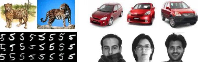
Another difficulty in addressing object recognition is that its current application often deals with a large number of categories. While designing more robust visual features and their corresponding similarity measures has gained signifi-cant progress, e.g. [1,15,17,19,22], the general conclusion is that no single feature is sufficient for handling diverse objects of broad categories. Take, for example, the four ob-ject classes in Figure1. To separate the images in jaguar
Figure 1. Examples from4 different object categories: jaguar, red car, handwritten digit, and human face. A typ-ical system for recognizing objects from the four categories most likely requires the use of several visual feature cues.
category from the others, keypoint-based features [15,20] should be useful, because only those jaguar images com-monly share the distinguishable patches in the skin area. On the other hand, color-based, e.g., [17] and shape-based fea-tures, e.g., [1] would be a reasonable choice for describing red carand handwritten digit, respectively. As for the human face category, it may require some proper combination of several visual features to yield a good rep-resentation. The example suggests that the goodness of a feature is often object-dependent.
Taking account of the foregoing considerations, we pro-pose a learning approach to designing ensemble kernel ma-chines with proper localization and regularization for object recognition. The use of ensemble kernels provides an ef-fective way of fusing various informative kernels resulted from assorted visual features and distance functions. Con-sequently, it allows our recognition method to work with a large number of object categories. The framework also matches the mechanism that human visual system can re-ceive various cues to perform recognition over diverse ob-ject classes. Even more crucially, in our formulation the learning of each ensemble kernel machine is done in a sample-dependentfashion. That is, there are as many num-ber of local ensemble kernels as the numnum-ber of training sam-ples. In testing a new sample, a locally adapted ensem-ble kernel can then be efficiently constructed by referencing those from the training data. We will demonstrate that the technique can significantly alleviate the effect of intraclass variations on the outcome of object recognition.
1.1. Related work
While image features for recognition can be constructed to locally or globally characterize objects of interest, their effectiveness may vary from application to application. For certain image retrieval problems, color-based histograms are conveniently adopted as a global descriptor, and shown to yield good results. For cases that they are not favorable, Pass et al. [17] propose to incorporate spatial information to form color coherence vectors (CCV). Recent trend toward resolving intraclass variations has popularized the design of local features, including region-based, part-based, and bag-of-features models [8]. Local feature models can also be improved by adding spatial information [24]. Yet another possibility, as suggested in Serre et al. [19], is to devise biologically-inspiredfilters to output features. In a related work of Mutch and Lowe [16], the biologically-motivated filters are further consolidated for recognition.
To enhance the recognition performance, it is natural to consider combining several information cues. Berg et al. [1] introduce the geometric blur feature by investigating both the appearance and distortion evidence. In [22], Varma and Zisserman propose to merge three kinds of filter banks to generate more informative textons for texture classification. Wu et al. [23] develop super-kernel to nonlinearly combine multimodal data for image and video retrieval. It is note-worthy that in each of the aforementioned methods only a single fusion model is established for all sample points.
Besides feature fusion, the idea to learn locally adap-tive classifiershas also been extensively explored. Aiming to boost nearest neighbor classification, Domeniconi and Gunopulos [7] derive a distance function for each training sample by re-weighting feature dimensions. For face recog-nition, Kim and Kittler [12] usek-means clustering to parti-tion data, and then learn an LDA classifier for each cluster. Their method alleviates the problems caused by that data may not be linearly separable and may violate the Gaussian assumption. In [5], Dai et al. consider a responsibility mix-ture model, in which each sample is associated with a value of uncertainty, and use an EM algorithm to combine local classifiers based on the uncertainty distribution.
More recently, Frome et al. [10] has established a frame-work that for each training image, a distance function is learned by combining multiple elementary ones. Since these local distances are learned independently, testing a new image requires a more elaborate nearest neighbor search. Besides, explicitly learning as many distance func-tions as training data may be less efficient.
1.2. Our approach
We address the problem of learning sample-dependent local ensemble kernels for object recognition over diverse categories. Our method is based on energy minimization
over an MRF model. Since a local learning approach some-times tends to be subject to curse of dimensionality and the effect of noisy data, we have taken account of these issues in designing the energy function. Specifically, we employ localized kernel alignment to obtain reasonable estimates, and build from them the observation data terms in the en-ergy function. A smoothness prior is also considered to in-corporate proper regularization to the model. The proposed framework can be efficiently solved by graph cuts, and does not suffer from the out-of-sample difficulty.
2. Information fusion via kernel alignment
Within a kernel-based classification framework such as SVMs, the underlying kernel matrix plays the role of infor-mation bottleneck: It records the inner product of each pair of training data in some high-dimensional feature space, and has a critical bearing on the resulting decision bound-ary. From the Mercer kernel theory [21], any symmetric and positive semi-definite matrix is a valid kernel, in which there exists one (and only one) corresponding embedding space for the data, and vice versa.
We intend to construct a number of kernel matrices, each of them corresponds to a specific type of image fea-ture. Combining features is thus equivalent to fusing nel matrices. To this end, we explore the concept of ker-nel alignmentintroduced by Cristianini et al. [4]. Consider now a two-class labeled dataset S = {(xi, yi)}`i=1 with
yi ∈ {+1, −1}. The kernel alignment between two kernel
matricesK1andK2overS is defined by
ˆ A(S, K1, K2) = hK1, K2iF phK1, K1iFhK2, K2iF , (1) wherehKp, KqiF =P ` i,j=1Kp(xi, xj)Kq(xi, xj). With
(1), the goodness of a kernel matrix K with respect to S can be measured by the alignment score, denoted as
ˆ
A(S, K, G), with a task-specific ideal kernel G = yyT
where y= [y1, ..., y`]T.
Based on the principle of alignment to a target kernel, Lanckriet et al. [13] propose the following procedure to learn a kernel matrix for classification. First, a set of kernel matrices are generated by using different kernel functions, or by tuning different parameter values. Then, semi-definite programming(SDP) for maximizing the alignment score is performed to derive the optimal kernel as a weighted com-bination of the generated kernel matrices. The resulting ker-nel gives good performance in their experiments.
2.1. Feature fusion over kernel matrices
Suppose the set of training samples hasC classes, i.e., S = {(xi, yi)}`i=1,yi ∈ {1, 2, . . . , C}. For each xi ∈ S,
from employing various visual features. It follows that for 1 ≤ r ≤ M
• The rth representation of sample xiis denoted as xri.
• dr: Xr× Xr
→ R is the rth distance measure, where Xr
denotes therth representation domain.
Note that the representations could differ significantly. An xi can be depicted by a histogram [22], a feature
vec-tor [12], a bag of feature vectors [15], or even a tensor. Such flexibility complicates the formulation of casting the problem of feature fusion. Several recent approaches, e.g., [10,23,24] have suggested to perform information fusion in the domain of distance functions. However, a distance function can be a metric or non-metric, and the range and scale of output values by different distance functions may also vary a lot. All these issues must be well addressed to make sure if feature fusion is reasonably done.
We instead consider information fusion in the domain of kernel matrices. For each representationr of the dataset S and the correspondingdr, we construct a “kernel function”,
similar to radial basis function (RBF) by varying the dis-tance measure, to generate therth kernel matrix, denoted asKr. (Note that the parameter, i.e., the variance in RBF
function can be tuned by cross validation.) Care must be taken whendr is not a metric because the resultingKr is
not guaranteed to be positive definite. Nevertheless, this is-sue can be resolved by the techniques suggested in [18,24]. LetΩ = {K1, K2, . . . , KM} be the kernel bank derived by
the above procedure. We define the target kernel matrixG for the multiple-category object recognition problem as
G(i, j) = (
+1, if yi= yj,
−1, otherwise. (2) Now multiclass feature fusion over the kernel bankΩ can be achieved by kernel alignment with respect to the target kernelG defined in (2). In particular, we follow the formu-lation in Lanckriet et al. [13] to solve
max α ˆ A(S, K, G) (3) subject to K = M X r=1 αrKr, trace(K) = 1, αr≥ 0, for 1 ≤ r ≤ M .
Alternatively, Hoi et al. [11] show that the optimiza-tion problem in (3) can be more efficiently solved using quadratic programmingafter reducing (3) into the
follow-ing equivalent formulation: min
α
αDTDα (4)
subject to vec(G)TDα = 1,
αr≥ 0, for 1 ≤ r ≤ M ,
wherevec(A) is the column vectorization of matrix A, and D = [vec(K1) vec(K2) . . . vec(KM)].
Thus far we have described how to fuseM visual cues through kernel alignment. An optimal α of (3) or (4) uniquely determines an ensemble kernelK =PM
r=1α
rKr
. Since the derivation does not involve any local property and considers all samples, the resulting kernelK is termed a global ensemble kernel. In this paper, we learn the SVM classifier by specifyingK. And we find that in our experiments such a global ensemble kernel machine in-deed achieves better recognition performance than any other SVM classifiers based on a single kernel fromΩ. Still, as we shall discuss in next section, the classification power can be further boosted by learning local ensemble kernels.
3. Learning local ensemble kernels
The previous section introduces a general principle for fusing features. Although it does provide a unified way of globally combining different feature representations, the ap-proach is too general to account for the interclass and intra-class variations in a complex object recognition problem.
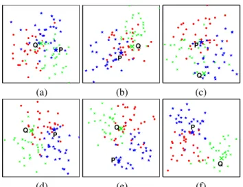
To illustrate the above point, we consider the example in Figure2. There we have a dataset of three classes (indicated by their color), and adopt three feature representations. That is, the kernel bankΩ = {Ka, Kb, Kc}. The respective
fea-ture spaces induced byKa,Kb, andKcare (conceptually)
plotted in Figures2a–2c. The resulting feature space by the global kernelK1= (Ka+ Kb+ Kc)/3, formed by a
uni-form combination overΩ is depicted in Figure2d. While K1can cause a better separation among the three classes of
data, it tends to misclassify samplesP and Q. Thus it ap-pears that a local learning scheme for constructing ensemble kernels may be beneficial. In Figure2e, the local ensemble kernelK2= (Ka+ Kb)/2 should be effective for
perform-ing classification aroundP . Similar effect can be found for K3= (Kb+ Kc)/2 around Q, as shown in Figure2f.
Thus, motivated by the example, and more importantly by the intrinsic difficulty in solving the recognition prob-lem, we consider a learning formulation for constructing local classifiers. Namely, our method would derive a local ensemble kernel machine for each training sample.
3.1. Initialization via localized kernel alignment
In learning local ensemble kernels, intuitively one can try to generalize the idea of kernel alignment to localized kernel alignment. As it turns out, the approach would give
P Q P Q P Q (a) (b) (c) P Q P Q P Q (d) (e) (f)
Figure 2. Six feature spaces correspond to six kernels (a) Ka, (b) Kb , (c) Kc , (d) K1= 1 3(K a +Kb +Kc ), (e) K2= 1 2(K a +Kb ), and (f) K3= 1 2(K b + Kc
). See text for further details.
satisfactory results. Nevertheless we only use them as the initial observations to our proposed optimization framework for reasons that will become evident later.
We first introduce the notion of neighborhood for each sample xi. Recall that the rth representation of xi is
xri, and the distance function isdr. The neighborhood of
xi can be specified by a normalized weight vector wi =
[wi,1, . . . , wi,`], where
wi,j = 1 M(w 1 i,j+ w2i,j+ · · · + w M i,j) (5) wr i,j = exp (−[dr(xri,xrj)]2 σr ) P` k=1exp ( −[dr(xr i,xrk)]2 σr ) . (6)
We then define the local target kernel of xiaccording to wi
as follows:
Gi(p, q) = wi,p× wi,q× G(p, q), for 1 ≤ p, q ≤ `. (7)
By replacing G with Gi in (3) and (4), we complete the
formulation of localized kernel alignment. The new con-strained optimization now yields an optimal vector αiand
therefore a local ensemble kernelKifor each sample xi.
Note that in (7) a weight distribution is dispersed over the local target kernelGisuch that whenever an element of
Girelates to more relevant samples in the neighborhood of
xi, it will have a larger weight (according to (5) and (6)).
This property enables the resulting kernelKi = P αriKr
to be formed by emphasizing thoseKr∈ Ω that their
cor-responding visual cues can more appropriately describe the relations between xi and its neighbors. Meanwhile,σr in
(6) can be used to control the extent of locality around xi.
To ensure a consistent way of specifying a neighborhood for each representation xr
i, we adopt the following scheme:
Fixing some values of, say,s and t, we adjust the value of σr
by binary search such that the nearests neighbors of xi,
using distancedr, will take upt% of the total weight of w i.
3.2. Local ensemble kernel optimization
There are two main reasons to look beyond the local ensemble kernels generated by kernel alignment. First, in most of the local learning approaches, e.g., [5,10,12] the resulting classifiers are determined by a relatively limited number of training samples from the neighborhood or some local group. They are sometimes sensitive to curse of di-mensionality, or at the risk of overfitting caused by noisy data. To ease such unfavorable effects, we prefer a local solution with proper regularization. Second, although the kernel alignment technique in (1) has its own theoretical merit [4], we find that it does not always precisely reflect the goodness of a kernel matrix. In our empirical testing, kernel matrices that better align to the target kernel may fail to achieve better classification performance.
To address the above two issues, we construct an MRF graphical model(V, E) for learning local ensemble kernels. For each sample xi, we create an observation node oiand
a state node βi. And for each pair of oiand βi, an edge is
connected. In addition if xjis one of thec nearest neighbors
of xi according to (5), an edge will be created between βi
and βj. Hence|V | = 2` and |E| ≤ (c + 1)`. Thus there are
two types of edges: E1 includes edges connecting a state
node to its observation node, andE2comprises those
link-ing two state nodes. ClearlyE = E1∪ E2. With the MRF
so defined, we consider the following energy function: E({βi}) = X (i,i)∈E1 Vd(βi, oi) + X (i,j)∈E2 Vs(βi, βj). (8)
On designing Vd(βi, oi). In general the data term Vd
should incorporate observation evidence at xi. Specifically,
we consider the neighborhood relation of xi specified by
(5) and the αi derived by localized kernel alignment. For
the ease of algorithm design, the total number of possi-ble states should be controlled within a manageapossi-ble range. We therefore runk-medoids clustering (based on the align-ment score) to divide{αi}`i=1 into n clusters, denoted as
{ ˆαp}np=1. (n = 50 in all our experiments.) The
map-ping αi 7→ ˆαp(i) is used to describe that αi is assigned
to the p(i)th cluster, and its vector value is approximated byαˆp(i). Consequently,Ki =PMr=1αriKris replaced by
ˆ Kp(i) =P M r=1αˆ r p(i)K r
. In the MRF graph each observa-tion node oi can now be set toαˆp(i). With these
modifica-tions, we are ready to defineVdas follows:
Vd(βi= ˆαq, oi= ˆαp(i)) = `
X
j=1
where1{·}is an indicator function, andfq(xj) is the result
of leave-one-out (LOO) SVM using kernel ˆKq (removing
thejth row and column) on xj. In practice, implementing
the LOO setting in (9) is too time-consuming. Nevertheless, it can be reasonably approximated by the following scheme: Each LOO testing on xjcan be carried out by applyingfqto
xj with the constraint that xjcannot be one of the support
vectors. (If xjis a support vector, then remove it fromfq.)
On designing Vs(βi, βj). We adopt the Potts model to
makeVsa smoothness prior in (8) on the free variable space.
The regularization would enrich our kernel learning formu-lation against noisy data. Specifically, we have
Vs(βi = ˆαqi, βj= ˆαqj) = 0, if qi= qj, t, else if yi6= yj, P × t, otherwise, (10)
wheret is a constant penalty, and constant P ≥ 1 is used to increase penalty between state nodes βi and βj whose
samples belong to the same object category.
With (9) and (10), the energy function in (8) is fully spec-ified. Since finding the exact solution to minimizing (8) is NP-hard, we apply graph cuts [2] to approximating the op-timal solution. Let{β∗i = ˆαp∗(i)} be the outcome derived by graph cuts. Then the optimal local ensemble kernel of xi
learned with (8) isK∗
i =
PM
r=1αˆrp∗(i)K
r. In testing, given
a test sample z, we can readily locate the nearest xi to z
by referencing (5), and use SVM with the local ensemble kernelK∗
i to perform classification.
4. Visual features and distance functions
We briefly describe the image representations and their corresponding distance functions used in our experiments. These features are chosen to capture diverse characteristics of objects, such as shape, color, and texture. And our ex-pectation is to use them to construct a kernel bankΩ that is rich enough for generating good ensemble kernels for rec-ognizing objects of various categories. Note that hereafter a term marked in bold font is to denote a pair of an image representation and its distance measure.
4.1. Geometric blur
Shape-based features can provide strong evidence for ob-ject recognition, e.g., [1,10,15]. We adopt the geometric blur descriptor proposed by Berg et al. [1]. The descriptor summarizes the edge responses within an image patch, and is relatively robust (via employing a spatially varying ker-nel) to shape deformation and affine transformation. Since the optimal kernel scale can depend on several factors, e.g., the object size, we implement geometric blur descriptors with two kernel scales, and denote them as GB-L and GB-S
respectively. Our implementation of geometric blur follows (2) of [24], in which spatial information is used.
4.2. Texton
Roughly speaking, texture feature refers to those image patterns that display homogeneity. To capture such visual cues, we consider the setting of [22], where99 filters from three filter banks are used to generate the textons (the vo-cabularies of texture prototypes [14]). An image can then be represented by a histogram that records its probability distribution over all the generated textons. Like in [14,22], theχ2distance is selected as the similarity measure.
4.3. SIFT
We use the SIFT (Scale Invariant Feature Transform) de-tector [15] to find interest points in an image. To mea-sure the distance between two images, vector quantiza-tion, as suggested in [20], is applied to transform a bag-of-features representation to a single feature vector via clus-tering. Since the number of clusters can critically affect the performance, we implement two different settings: The numbers of clusters are set to 2000 (SIFT-2000) and 500 (SIFT-500) respectively. We also normalize the feature vec-tor of each image to a distribution, and again use the χ2
distance as the similarity measure.
4.4. Biologically-motivated feature
Serre et al. [19] propose a set of features that emu-lates the visual system mechanism. Through a four-layer (known as S1, C1, S2, and C2) hierarchical processing, an image can be expressed by a set of scale and translation-invariant C2 features. Motivated by their good performance for recognition, we use the C2 features as one of our image representations in the experiments. For this representation, Euclidean distance is applied to measuring the dissimilarity between a pair of images.
4.5. Color related feature
The visual features described so far catch characteristics only based on gray-level information. We thus further con-sider color-related image features, especially those which have compact representations and match human intuition. Specifically, we use a 125-bin color histogram (CH) ex-tracted from the HSV color space to represent an image. To include spatial information, the250-bin color coherence vector (CCV) [17] is also implemented. After normalizing a CH or CCV of an image to a distribution, Jeffrey diver-genceis used as the distance function.
5. Experimental results
A real-world recognition application often involves ob-jects from diverse and broad categories. Even for obob-jects
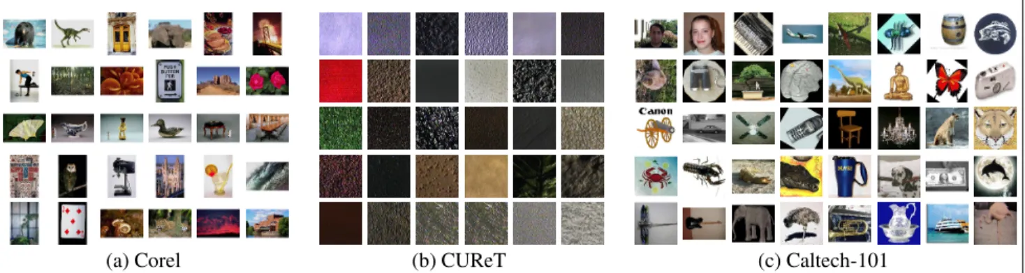
(a) Corel (b) CUReT (c) Caltech-101
Figure 3. 100 image categories. (a) 30 categories from Corel, (b) 30 categories from CUReT, and (c) 40 categories from Caltech-101.
from the same category, their appearances and characteris-tics can still vary due to different poses, scales, or light-ing conditions. Nonetheless, a problem like this serves as a good test bed for evaluating the proposed local ensemble kernel learning. In our implementation, we formulate the recognition task as a multiclass classification problem, and use LIBSVM [3], in which one-against-one rule is adopted, to learn the classifiers with the kernel matrices produced by our method. We carry out experiments on two sets of im-ages. The first one is Caltech-101 collected by Fei-Fei et al. [9], and the second set is a mixture of images from Corel, CUReT [6] and Caltech-101. Detailed experimental results and discussions are given below.
5.1. Caltech-101 dataset
The Caltech-101 [9] dataset consists of101 object cate-gories and an additional class of background images. Each category contains about 40 to 800 images. Although ob-jects in these images often locate in the central regions, the total number of categories (i.e., 102) and large intraclass variation still make this set a very challenging one. Some examples are shown in Figure3c.
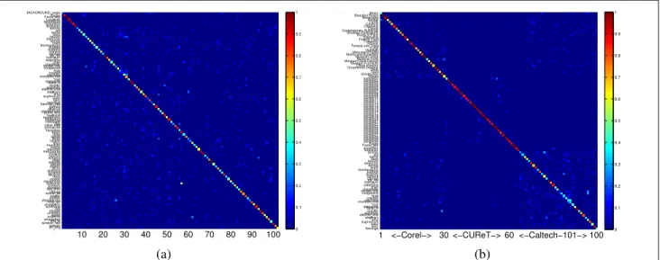
As the sizes of images in this set are different and some of our adopted image representations are sensitive to this is-sue, we resize each image into a resolution around300 × 200. (The aspect ratio is maintained.) For the sake of com-parison, our experiment setup is similar to the one in Berg et al. [1] and Zhang et al. [24]. Namely, we randomly select30 images from each category: 15 of them are used for train-ing and the rest are used for testtrain-ing. However, in [10], the class of background images (i.e., BACKGROUND Google) is excluded from the experiments. We thus include both the two settings in our experiments, and denote them as with-backgroundand without-background. The quantitative sults and the confusion table of testing Caltech-101 are re-ported in Table1and Figure4a, respectively. In Table1, the exact meanings of the abbreviations for the eight kinds of image representations, listed in the Rep.-r column, have been described in Section 4. In the Method column, we
Table 1. Recognition rates for Caltech-101.
Caltech-101 dataset Method Rep.-r With-background Without-background GB-L 51.57 % 51.95 % GB-S 53.40 % 53.86 % Texton 20.73 % 20.99 % SIFT-2000 28.76 % 29.31 % SIFT-500 23.86 % 24.29 % C2 31.37 % 31.68 % CH 13.66 % 13.80 % Kr CCV 15.10 % 15.25 % K All 54.38 % 54.92 % Ki All 57.25 % 57.95 % K∗ i All 59.80 % 61.25 %
specify what kind of kernel matrix is used with SVM to form a kernel machine: Krmeans the kernel (inΩ) with
respect to the representation xr is used, and analogously K, KiandKi∗ indicate the use of an ensemble kernel
de-rived by solving global kernel alignment (4), localized ker-nel alignment (7), and MRF optimization (8), respectively.
The performance gain by our technique is significant. Despite our implementation of geometric blur is less effec-tive (the GB-L and GB-S entries in Table1) than those re-ported in [24], the proposed ensemble kernel learning can still achieve state-of-the-art recognition rates.
5.2. Corel + CUReT + Caltech-101 dataset
In testing with Caltech-101 dataset, we observe that the performance of geometric blur descriptor [1] is noticeably dominant. This phenomenon generally causes the resulting ensemble kernel is not uniformly combined, and therefore the advantage of our method may not be fully exploited. We thus construct a second dataset by collecting images from different sources to further increase the data variations.
We first select30 image categories from the Corel im-age database, which is widely used in the research of imim-age
BACKGROUNDGoogle Faces FacesLeopardseasy
Motorbikesaccordion airplanesanchorant barrelbass beaver binocularbonsaibrain brontosaurusbuddhabutterfly camera cannoncarside ceilingfan
cellphone chair chandelier cougarcougarbfodyace crab crayfish crocodile crocodileheadcup dalmatiandragonflydollardolphinbill
electriceuphoniumelephantguitaremu ewer ferry flamingo flamingogerenukgarfieldhead
gramophoneheadphonegrandhedgehoghawksbillpiano
helicopteribis inlineskate joshuakangarooketchtree
lamp laptop llama lobsterlotus mandolinmayfly menorah metronomeminaretnautilus octopusokapi pagoda panda pigeon pizza platypuspyramid revolverroosterrhino saxophoneschoonerscissors scorpion seasnoopyhorse
soccerstaplerball
starfish stegosaurusstrawberrysunflowerstopstickign trilobite umbrellawaterwatchlilly
wheelchairwildcat windsoryinwrenchcyhairang
10 20 30 40 50 60 70 80 90 100 0 0.1 0.2 0.3 0.4 0.5 0.6 0.7 0.8 0.9 1 Bears
Beautiful RosesBeveragesBonsai Cards Caverns CheetahsClouds Contemporary Buildings Dinosaur IllustrationsDoors of Paris Elephants Festive FoodFireworks Fitness Forests and Trees Fungi Highway Monument Valley Moths and ButterfliesMuseum China Museum Dolls Museum Duck Decoys Museum FurnitureOffice Interiors Ornamental Designs Owls Tools UniversitiesWaves sample01 sample02 sample03 sample04 sample05 sample06 sample07 sample08 sample09 sample10 sample11 sample12 sample13 sample14 sample15 sample16 sample17 sample18 sample19 sample20 sample21 sample22 sample23 sample24 sample25 sample26 sample27 sample28 sample29 sample30Faces Faceseasy accordionairplanes anchorbarrelant bass beaver binocularbonsai brain brontosaurusbuddha butterflycamera cannoncarside
ceilingfan cellphonechair chandelier cougarbody cougarface crab crayfish crocodile crocodiledalmatiandollarheadcupbill dolphin dragonfly electricguitar elephant emu euphoniumewer ferry flamingo
1 <−Corel−> 30<−CUReT−>60 <−Caltech−101−>100 0 0.1 0.2 0.3 0.4 0.5 0.6 0.7 0.8 0.9 1 (a) (b)
Figure 4. The confusion tables by our method on two different datasets. (a) Caltech-101. (b) Corel + CUReT + Caltech-101.
retrieval. Images in the same category share the same se-mantic concept, but still have their individual variety. To illustrate, images from each of the30 categories are shown in Figure3a. We then collect the first30 texture categories from CUReT [6] database. Texture images within a cate-gory are pictured for the same material under various view-ing angles and illumination conditions. Similar to [22], we crop the central200 × 200 texture region of each image, and convert it to grayscale. However unlike in [22], we do not normalize the intensity distribution to zero mean and unit standard deviation in that this pre-processing is not ap-plied to images from the other two sources. Figure3b gives an overview of the 30 categories selected from CUReT. Finally, we choose40 object categories from Caltech-101 dataset according to their alphabetical order. (Note that the background category is excluded.) These categories are in-deed those shown in Figure3c. In total the resulting dataset from the three sources has100 image categories.
Similar to the setting in Section 5.1, we randomly select 30 images from each category. Half of them are used for training, and the rest are used for testing. The quantitative results and the confusion table are shown in Table2and Fig-ure4b, respectively. In Table2, there are four recognition rates recorded for each scheme. The first three are evalu-ated by considering only samples within specific datasets, and the last is computed by taking all samples into account. From Table2and Figure4b, we have the following ob-servations: 1) In the Corel database, several image repre-sentations can achieve comparable performance, and tend to complement each other. Thus all the three schemesK, KiandKi∗that combine various features achieve
substan-tial improvements. 2) Unlike testing with Caltech-101, the optimal feature combinations for classifying objects in the combined dataset are more diversely distributed. Thus the
accuracy improvement of the schemeK that globally learns a single fusion of visual features for all samples is relatively limited, compared with those by the two local schemesKi
andK∗
i. 3) No matter using which dataset, the performance
of our approach is better than the best performance obtained from using a single image representation. This means that our method can effectively select good feature combination for each sample, and thus improve the recognition rates. Complexity analysis. Most of the time complexity in training is consumed by the construction of the kernel bank Ω. It involves the pairwise distance calculations, and some of our chosen distances require extensive computation time. For 1500 training samples, this step would take several hours to complete. In addition, after kernels are grouped as clusters in the MRF optimization, learning the sample-dependent SVM classifiers can be done in less than2 min-utes. In testing a novel sample, our method carries out near-est neighbor search to locate the appropriate local classifier and then performs the classification. Totally, it would take about51
2 minutes for testing a new sample. Finally, we
re-mark that although a local kernel is learned for each train-ing sample, we do not need to store the whole kernel matrix but the ensemble weights. Hence there is no extra space requirements due to our proposed method.
6. Conclusions
Motivated by that the best visual feature combination for classification could vary from object to object, we have in-troduced a sample-dependent learning method to construct ensemble kernel machines for recognizing objects over broad categories. Overall, we have strived to demonstrate such advantages with the proposed optimization framework
Table 2. Recognition rates for Corel + CUReT + Caltech-101.
Corel + CUReT + Caltech-101 dataset Method Rep.-r
Corel (30 classes) CUReT (30 classes) Caltech (40 classes) ALL (100 classes)
GB-L 59.91 % 70.36 % 52.30 % 60.00 % GB-S 62.14 % 75.47 % 53.30 % 62.60 % Texton 53.33 % 88.89 % 23.67 % 52.13 % SIFT-2000 45.56 % 83.56 % 30.00 % 50.73 % SIFT-500 42.00 % 83.56 % 25.83 % 48.00 % C2 48.22 % 59.78 % 30.00 % 44.40 % CH 55.33 % 24.22 % 16.17 % 30.33 % Kr CCV 56.44 % 33.78 % 17.47 % 34.13 % K All 75.78 % 86.00 % 46.17 % 67.00 % Ki All 76.67 % 92.89 % 55.83 % 73.20 % K∗ i All 77.33 % 92.67 % 59.33 % 74.73 %
over an MRF model, of which we are able to use kernel alignment to give good initializations, and also with the promising experimental results on two extensive datasets. Acknowledgements. This work is supported in part by grants 95-2221-E-001-031 and 96-EC-17-A-02-S1-032.
References
[1] A. Berg, T. Berg, and J. Malik. Shape matching and object recognition using low distortion correspondences. In CVPR, pages 26–33, 2005. 1,2,5,6
[2] Y. Boykov, O. Veksler, and R. Zabih. Fast approximate en-ergy minimization via graph cuts. PAMI, 23(11):1222–1239, 2001. 5
[3] C.-C. Chang and C.-J. Lin. LIBSVM: A Library for Support Vector Machines, 2001. Software available at http://www.csie.ntu.edu.tw/∼cjlin/libsvm. 6
[4] N. Cristianini, J. Shawe-Taylor, A. Elisseeff, and J. Kandola. On kernel-target alignment. In NIPS, 2001. 2,4
[5] J. Dai, S. Yan, X. Tang, and J. Kwok. Locally adaptive clas-sification piloted by uncertainty. In ICML, pages 225–232, 2006. 2,4
[6] K. Dana, B. Van-Ginneken, S. Nayar, and J. Koenderink. Re-flectance and texture of real world surfaces. ACM Trans. on Graphics, 18(1):1–34, 1999. 6,7
[7] C. Domeniconi and D. Gunopulos. Adaptive nearest neigh-bor classification using support vector machines. In NIPS, 2001. 2
[8] G. Dork´o and C. Schmid. Selection of scale-invariant parts for object class recognition. In ICCV, pages 634–640, 2003. 2
[9] L. Fei-Fei, R. Fergus, and P. Perona. Learning generative visual models from few training examples: An incremental bayesian approach tested on 101 object categories. In CVPR Workshop on Generative-Model Based Vision, 2004. 6 [10] A. Frome, Y. Singer, and J. Malik. Image retrieval and
clas-sification using local distance functions. In NIPS, 2006. 2, 3,4,5,6
[11] S. Hoi, M. Lyu, and E. Chang. Learning the unified kernel machines for classification. In KDD, pages 187–196, 2006. 3
[12] T.-K. Kim and J. Kittler. Locally linear discriminant analysis for multimodally distributed classes for face recognition with a single model image. PAMI, 27(3):318–327, 2005. 2,3,4 [13] G. Lanckriet, N. Cristianini, P. Bartlett, L. Ghaoui, and
M. Jordan. Learning the kernel matrix with semi-definite programming. In ICML, pages 323–330, 2002. 2,3 [14] T. Leung and J. Malik. Representing and recognizing the
visual appearance of materials using three-dimensional tex-tons. IJCV, 43(1):29–44, 2001. 5
[15] D. Lowe. Distinctive image features from scale-invariant keypoints. IJCV, 60(2):91–110, 2004. 1,3,5
[16] J. Mutch and D. Lowe. Multiclass object recognition with sparse, localized features. In CVPR, pages 11–18, 2006. 2 [17] G. Pass, R. Zabih, and J. Miller. Comparing images using
color coherence vectors. In ACM MM, pages 65–73, 1996. 1,2,5
[18] E. Pekalska, P. Paclik, and R. Duin. A generalized ker-nel approach to dissimilarity-based classification. JMLR, 2(2):175–211, 2002. 3
[19] T. Serre, L. Wolf, and T. Poggio. Object recognition with fea-tures inspired by visual cortex. In CVPR, pages 994–1000, 2005. 1,2,5
[20] J. Sivic and A. Zisserman. Video google: A text retrieval ap-proach to object matching in videos. In ICCV, pages 1470– 1477, 2003. 1,5
[21] V. Vapnik. Statistical Learning Theory. Wiley, 1998. 2 [22] M. Varma and A. Zisserman. A statistical approach to
tex-ture classification from single images. IJCV, 62(1-2):61–81, 2005. 1,2,3,5,7
[23] Y. Wu, E. Chang, K. Chang, and J. Smith. Optimal mul-timodal fusion for multimedia data analysis. In ACM MM, pages 572–579, 2004. 2,3
[24] H. Zhang, A. Berg, M. Maire, and J. Malik. SVM-KNN: Discriminative nearest neighbor classification for visual cat-egory recognition. In CVPR, pages 2126–2136, 2006. 2,3, 5,6