應用於進位儲存加法器式多常數乘法設計面積最小化之智慧型正負號延伸及精確位元計算技術

國立交通大學

電子工程學系 電子研究所

碩 士 論 文

應用於進位儲存加法器式多常數乘法設計面積

最小化之智慧型正負號延伸及精確位元計算技

術

Area Minimization for CSA-Based Multiple Constant

Multiplication Designs using Smart Sign Extension and

Accurate Bit Counting

研究生：林子敬

指導教授：黃俊達 博士

應用於進位儲存加法器式多常數乘法設計面積

最小化之智慧型正負號延伸及精確位元計算技

術

Area Minimization for CSA-Based Multiple Constant

Multiplication Designs using Smart Sign Extension and

Accurate Bit Counting

研究生：林子敬 Student: Lin, Tzu-Ching

指導教授：黃俊達 博士 Advisor: Dr. Huang, Juinn-Dar

國立交通大學

電子工程學系 電子研究所

碩士論文

A Thesis

Submitted to Department of Electronics Engineering & Institute of Electronics College of Electrical and Computer Engineering

National Chiao Tung University in Partial Fulfillment of the Requirements

for the Degree of Master of Science

in

Electronics Engineering & Institute of Electronics

November 2013

Hsinchu, Taiwan, Republic of China

i

應用於進位儲存加法器式多常數乘法設計面積最小化

之智慧型正負號延伸及精確位元計算技術

研究生：林子敬 指導教授：黃俊達 博士

國立交通大學

電子工程學系 電子研究所碩士班

摘要

在眾多用於訊號處理的特殊應用積體電路 (ASIC)中，比如有限脈衝響應濾波 器(FIR filter) 、無限脈衝響應濾波器(IIR filter) 、離散餘弦轉換 (DCT) 和快速傅立葉轉換(FFT)，多常數乘法是一項廣泛用於取代一般乘法器的做法。 只用加法器、減法器和平移的多常數乘法模組可以大幅度減少硬體面積。對高速 的應用而言，因為基於進位傳遞加法器 (carry propagation adder)的多常數乘 法有著冗長的進位傳遞，所以基於進位儲存加法器(carry save adder)的架構的 多常數乘法就發展出來。目前的基於進位儲存加法器的架構的多常數乘法只發展 到將進位儲存加法器的數量最佳化，卻忽略了每個進位儲存加法器在實作上的差 異。然而，不像進位傳遞加法器，一般的正負號延伸 (sign extension)並不適 用於進位儲存加法器。而且，在每個進位儲存加法器之間，字元長度的變異性是 很強烈的。在本篇論文中，我們提出一個叫做智慧型正負號延伸的系統化的正負 號延伸方法來減少字元長度。將其和精確位元計算技術結合後，再用整數線性規 畫(ILP)來做多常數乘法設計的面積最佳化。實驗結果顯示，和傳統的多常數方 法比較，面積的改善幅度最高可達 30%。

ii

Area Minimization for CSA-Based Multiple Constant

Multiplication Designs using Smart Sign Extension and

Accurate Bit Counting

Student: Lin, Tzu-Ching Advisor: Dr. Huang, Juinn-Dar

Department of Electronics Engineering & Institute of Electronics

National Chiao Tung University

Abstract

Multiple constant multiplication (MCM) method is widely adopted as a replacement of general purpose multiplier in many ASIC signal processing systems such as FIR filter, IIR filter, DCT and FFT. The MCM block that consists only adders, subtractors and shifters can reduce area cost significantly. For high-speed applications, carry save adder (CSA) based MCM is proposed because the long carry propagation path in traditional carry propagation adder (CPA) is reduced. Currently, all published algorithms of CSA-based MCM problem only count to word level without touching the details of implementation. However, unlike CPA, trivial sign extension is not suitable for CSA. Also, the word length variation in different CSA's is large. In this thesis, we propose a new systematic method called smart sign extension to reduce adder bits and combine it with accurate bit counting while doing MCM area optimization by an ILP (Integer Linear Programming) tool. Experimental results show an area improvement up to 30% compared to the conventional MCM method.

iii

Acknowledgement

首先我要感謝上天及父母賜與我生命並讓我繼續活著，畢竟只有活人才有辦 法進行研究。雖然不曉得有生之年能不能報答如此大恩，還是努力試試看吧。 再來，感謝指導教授黃俊達教授一路下來的指導與栽培，總是在必要的時刻 提供寶貴的意見，來讓研究順利進行下去。在小組報告時對於報告需要的技巧與 細節都鉅細靡遺的指出需要改進的地方，這不是每位老師都有意願去做的，這對 於未來不論是工作方面或是日常處事都提供了足夠的訓練，讓人終生受用無窮， 真的是非常感謝。 另外，也感謝 413 實驗室雷永群學長一直以來的陪伴與協助，在研究課題遇 到瓶頸是總是大力協助，而且也抽出許多額外時間來幫忙進行研究與討論，真的 是十分感謝這一年多下來將近兩年的幫忙。還有，陳詣航學長和劉家宏學長對於 實驗室環境的打造與維護付出了相當的心血與努力，讓全實驗室的學生都能享受 優良的實驗與工作環境，這邊需要特別感謝他們兩位。也要感謝同一屆的偉豪、 建宇跟慧珊，和你們一起度過的這兩年相當愉快。尤其是偉豪跟建宇總是在我需 要的時候幫忙和陪伴，要是沒有兩位的大力協助，這兩年會有許多難關無法順利 突破吧。還有，實驗室的兩位學弟國政跟顥瀚，在我需要兩位協助時能排除萬能， 於危急存亡之時提供即時的幫忙，真的是非常感謝。 最後，感謝交大願意提供本人機會攻讀電子所系統組碩士，讓我能夠完成長 年以來的夢想，也要感謝國家與社會提供資源來讓交大的運作能夠順利進行。附 帶一提，對於在口試前來幫忙加油打氣，卻一時忘記名字的高中同學林肇尉說聲 對不起，我真的不是故意忘掉你名字的。 林子敬 謹誌 西元 2013 年 11 月 20 日 國立交通大學電子研究所

iv

Content

目錄

摘要 ...i Abstract ... ii Acknowledgement ... iii Content ... iv List of Tables ... vi

List of Figures ... vii

Chapter 1. Introduction ... 1

1.1 Multiple Constant Multiplication (MCM) ... 1

1.2 Introduction to MCM Algorithms ... 7

1.2.1 Common Subexpression Elimination (CSE) Algorithm ... 7

1.2.2 Graph Algorithm ... 9

1.3 MCM Using Carry Save Adder for Addition Implementation ... 13

Chapter 2. Previous Work ... 15

2.1 CPA-Based Algorithms ... 15

2.2 CSA-Based Algorithms ... 16

Chapter 3. Proposed Algorithm ... 18

3.1 Bit Level Area Optimization Using CSA-Based Structure ... 18

3.2 Problem Formulation ... 22

3.3 Overall Flow ... 22

3.4 Find AGN representations for Constants... 25

3.5 Construct Boolean Network ... 27

v

3.6.1 Calculation of Number of Adder Bits... 30

3.6.2 Smart Sign Extension ... 32

3.6.3 Bit Propagation for OR Operation ... 42

3.7 Transform Boolean Network to 0-1 ILP Problem ... 43

Chapter 4. Experimental Results ... 46

Chapter 5. Conclusion ... 52

vi

List of Tables

Table 1. General flow of graph algorithm ... 12

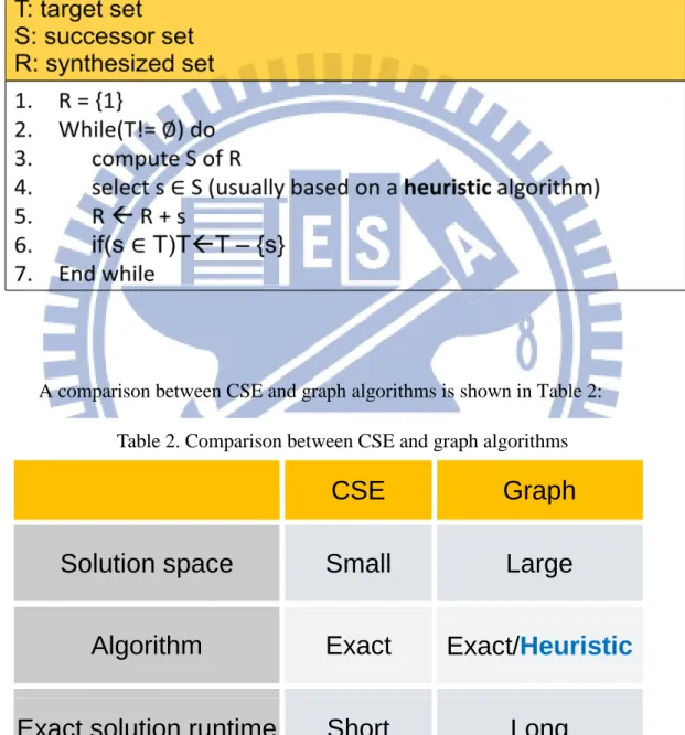
Table 2. Comparison between CSE and graph algorithms ... 12

Table 3. Overall process of finding legal AGN representations for all constants ... 27

Table 4. The truth table of –x5 – y5 and –2 + x5+ y5. ... 35

Table 5. The truth table of –1 +z4 and –z4 ... 36

Table 6. The MSB and LSB of both sum and carry in case 1 ... 36

Table 7. The MSB and LSB of both sum and carry in case 2 ... 38

Table 8. The MSB and LSB of both sum and carry in case 3 ... 40

Table 9. MSB and LSB of sum and carry as well as the number of adder bits for all three cases ... 41

Table 10. Definition of different techniques ... 47

Table 11. 10 FIR filters used in Exp.1 ... 47

Table 12. Comparison between Ref. and (a) ... 48

Table 13. Comparison between Ref. and (b) ... 49

Table 14. Comparison between Ref. and (a) + (b) ... 50

vii

List of Figures

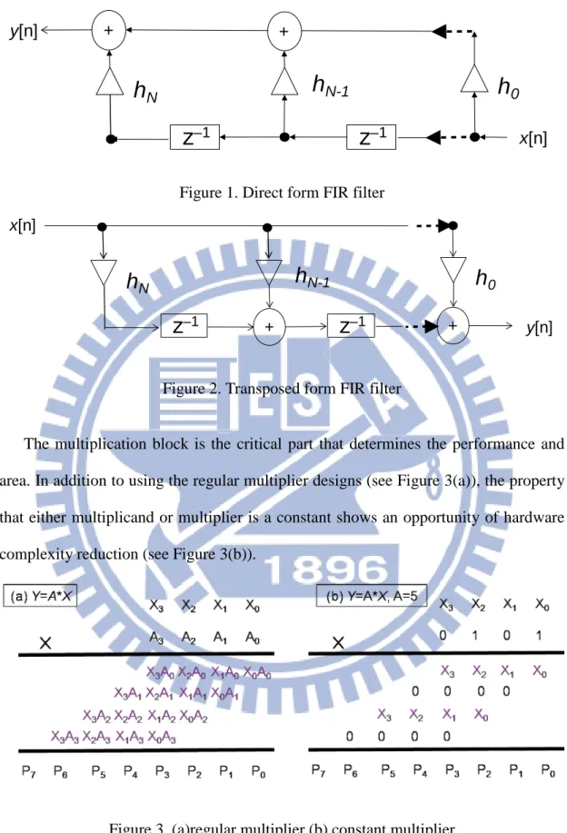
Figure 1. Direct form FIR filter ... 2

Figure 2. Transposed form FIR filter ... 2

Figure 3. (a)regular multiplier (b) constant multiplier ... 2

Figure 4. (a) without sharing, 5 additions (b) with sharing of 5x, 4 additions ... 4

Figure 5. (a) Carry propagation adder (CPA) (b) Carry save adder (CSA) ... 5

Figure 6. Comparison of CPA structures [1] ... 5

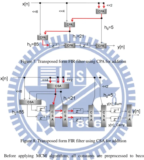
Figure 7. Transposed form FIR filter using CPA for addition ... 6

Figure 8. Transposed form FIR filter using CSA for addition ... 6

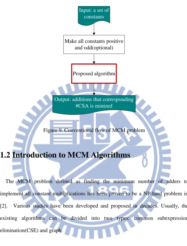
Figure 9. Conventional flow of MCM problem ... 7

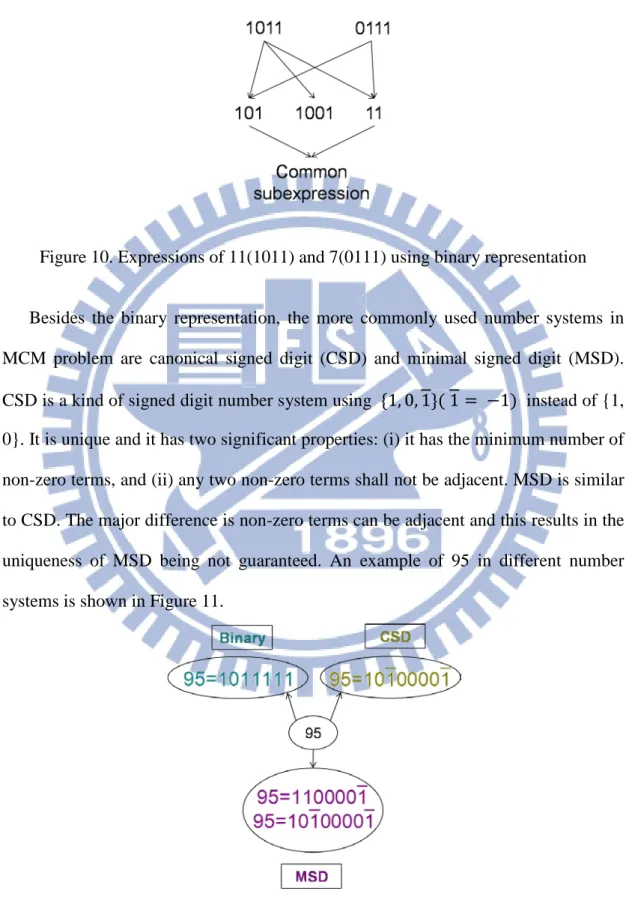
Figure 10. Expressions of 11(1011) and 7(0111) using binary representation ... 8

Figure 11. 95 in different number systems ... 8

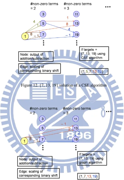
Figure 12. {7, 13, 19} solution of a CSE algorithm ... 10

Figure 13. {7, 13, 19} solution of a graph algorithm ... 10

Figure 14. (a) One graph solution of {39, 83} (b) 39<<2 + 5 under CSD representation ... 11

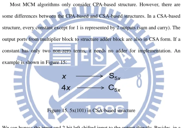
Figure 15. 5x(101) in CSA-based structure ... 13

Figure 16. 39<<1 + 5 using CPA or CSA ... 14

Figure 17. (a) Nset for general number (b) Nset for approximate general number ... 16

Figure 18. One input of each CSA must be 1 ... 17

Figure 19. Two different additions for implementing 51x have different the number of adder bits ... 18

Figure 20. An 8-bit two's complement number ... 19

Figure 21. MSB is a sign bit while the other bits are unsigned bits ... 20

Figure 22. (a) Trivial sign extension (b) Smart sign extension ... 21

Figure 23. Overall flow of our proposed algorithm ... 24

Figure 24. Legitimate AGN representations of 51 ... 26

Figure 25. Corresponding AND gate of −1 + 13<<2 ... 28

Figure 26. OR gate connected with all AGN representations for 51 ... 29

Figure 27. Part of the whole Boolean network ... 30

Figure 28. Calculation of #adder bits of v51_3 ... 32 Figure 29. (a) Sign extension for input x (b) Direct wiring (c) First step

viii

complete ... 33

Figure 30. Example of case 1 after sign extension ... 37

Figure 31. Example of case 2 after sign extension ... 39

Figure 32. Example of case 3 after sign extension ... 41

Figure 33.Example of Bit Propagation for OR operation ... 42

Figure 34. Boolean network with weighting in terms of number of adder bits ... 45

1

Chapter 1. Introduction

1.1 Multiple Constant Multiplication (MCM)

The FIR(finite impulse response) filter is one of the most important digital signal processing(DSP) application because its inherit stability and linear phase property which can be obtained easily by making the impulse response symmetric. The following equation is used to describe an FIR filter:

0

[ ]

* [

]

N i i

y n

h

x n i

=

=

∑

−

where y[n] is the filter output at time n, hi is the ith coefficient of the filter, x[n−i] is

input signal at time n−i, and N is the order of the filter. It can be implemented in the direct form, as shown in Figure 1, or in the transposed form, as shown in Figure 2. Compared to the direct form, the transposed form avoids the long adder chain, thus having higher throughput and parallelism. The transposed form FIR filter can be decomposed into two parts: one is called multiplier block, including the multiplications of the input signal with a set of constant coefficients, while the other is called structure adder, including the adders and registers, and its output is the weighted sum of inputs.

2

Figure 1. Direct form FIR filter

Figure 2. Transposed form FIR filter

The multiplication block is the critical part that determines the performance and area. In addition to using the regular multiplier designs (see Figure 3(a)), the property that either multiplicand or multiplier is a constant shows an opportunity of hardware complexity reduction (see Figure 3(b)).

Figure 3. (a)regular multiplier (b) constant multiplier

As shown in Figure 3(b), constant multiplication can be implemented by additions and bit shifts. For example:

+ y[n] x[n]

h

_N

h

N-1

h

₀

z

–1

_z

–1 + + + x[n] y[n]

h

_N

h

N-1

h

₀

z

–1

_z

–1

3 5x = x<<2 + x

Compared to a multiplier, this shift-and-add structure can significantly reduce area. Because bit shifts have no cost in ASIC design, the optimization problem of finding the smallest number of adders for the multiplication of single constant is called single constant multiplication (SCM) problem.

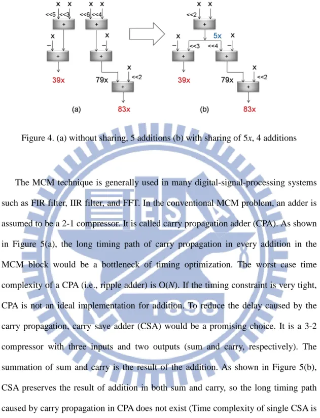
Furthermore, the common input and bit-pattern similarity between constants in the transposed form FIR filter provides the opportunity of sharing the intermediate addition results among different constant multiplications. The problem of minimizing the total number of adders in the structure of a single input multiplied with multiple constants is called multiple constant multiplications (MCM) problem. For example, the two constants 39 and 83 can be decomposed as:

39x = x<<5 + x<<3 − x

83x = x<<6 + x<<4 + x<<2 + x

They can be further reduced in the form of the following equations if 5x is shared in both equations:

39x = (x<<2 + x)<<3 − x

83x = (x<<2 + x)<<4 + x<<2 + x

The total number of additions is reduced from 5 to 4, as shown in Figure 4, if we find the intermediate results of additions properly.

4

Figure 4. (a) without sharing, 5 additions (b) with sharing of 5x, 4 additions

The MCM technique is generally used in many digital-signal-processing systems such as FIR filter, IIR filter, and FFT. In the conventional MCM problem, an adder is assumed to be a 2-1 compressor. It is called carry propagation adder (CPA). As shown in Figure 5(a), the long timing path of carry propagation in every addition in the MCM block would be a bottleneck of timing optimization. The worst case time complexity of a CPA (i.e., ripple adder) is O(N). If the timing constraint is very tight, CPA is not an ideal implementation for addition. To reduce the delay caused by the carry propagation, carry save adder (CSA) would be a promising choice. It is a 3-2 compressor with three inputs and two outputs (sum and carry, respectively). The summation of sum and carry is the result of the addition. As shown in Figure 5(b), CSA preserves the result of addition in both sum and carry, so the long timing path caused by carry propagation in CPA does not exist (Time complexity of single CSA is O(1)).

5

Figure 5. (a) Carry propagation adder (CPA) (b) Carry save adder (CSA)

If we use a faster CPA, the hardware cost will increase. A comparison of different CPA structures is shown in Figure 6. The CPA structures with timing complexity which is O(logN) has the greatest area complexity which is O(NlogN) in a single N-bit CPA. Compared to CSA, it has less chance to meet tight timing constraint with small area of MCM block.

Figure 6. Comparison of CPA structures [1]

Figure 7 and 8 shows two different structures for implementing an FIR filter. Figure 7 is the traditional structure using CPA for addition and Figure 8 shows the high-speed structure using CSA for addition in the transposed form FIR filter. For the high-speed structure, the CSA representation is maintained until summation of constants is done. Then an extra CPA is used to combine sum and carry into the FIR

6

output. However, the delay of critical path in Figure 7 is only the delay of three CPA's and the delay of critical path in Figure 8 is the delay of three CSA's.

Figure 7. Transposed form FIR filter using CPA for addition

Figure 8. Transposed form FIR filter using CSA for addition

Before applying MCM algorithms, all constants are preprocessed to become positive and odd, because any even constants can be generated by bitwise left shift of an odd constant and each negative constant can be replaced by positive one by using subtractor. Then, the problem definition becomes: given a set of constants, find the minimum number of adders for implementation of all constant multiplications. An illustration of conventional MCM problem flow is shown in Figure 9.

7 Input: a set of

constants

Make all constants positive and odd(optional)

Output: additions that corresponding #CSA is minized

Proposed algorithm

Figure 9. Conventional flow of MCM problem

1.2 Introduction to MCM Algorithms

The MCM problem defined as finding the minimum number of adders to implement all constant multiplications has been proven to be a NP-hard problem in [2]. Various studies have been developed and proposed in decades. Usually, the existing algorithms can be divided into two types: common subexpression elimination(CSE) and graph.

1.2.1 Common Subexpression Elimination (CSE) Algorithm

In computer science, an expression is a finite combination of symbols (constant, variable, operation, function, etc.). All expressions can be divided into subexpressions, which is a part of the original expression. If the same subexpression can be found between in expressions, this subexpression is called common subexpression. Figure

8

10 shows an example of expressions of 11 and 7 using binary representation and part of their corresponding subexpressions and common subexpressions:

Figure 10. Expressions of 11(1011) and 7(0111) using binary representation

Besides the binary representation, the more commonly used number systems in MCM problem are canonical signed digit (CSD) and minimal signed digit (MSD). CSD is a kind of signed digit number system using {1, 0, 1}( 1 = −1) instead of {1, 0}. It is unique and it has two significant properties: (i) it has the minimum number of non-zero terms, and (ii) any two non-zero terms shall not be adjacent. MSD is similar to CSD. The major difference is non-zero terms can be adjacent and this results in the uniqueness of MSD being not guaranteed. An example of 95 in different number systems is shown in Figure 11.

9

According to the pre-decided number representation, CSE algorithms first decompose all constants into subexpressions and then search for subexpressions of the target constants to find optimal sharing of addition results for saving the number of adders being used. For example, 39 = 101001 and 83 = 1010101 in CSD representation, where 101 = 510 is a common subexpression. There are four adders

that are used as shown in Figure 4(b). Selecting different number representation will affect the time complexity and solution quality of the CSE algorithm. Selecting CSD can save run time because of its uniqueness. On the other hand, selecting MSD enables larger design space and better solution quality. One disadvantages of CSE algorithms is that the implementation of numbers is restricted in decomposition. The decomposed number must be a subexpression of the original expression so that they cannot make use of the carry propagation for more sharing of addition results [3].

1.2.2 Graph Algorithm

Compared with the CSE algorithm, the graph-based algorithm removes the restriction on decomposition. A solution for implementing constants set = {7, 13, 19} provided by a CSE algorithm is shown in Figure 12. In Figure 12, the node is a constant product of input and edge is the scaling of binary shift. One intermediate result 5 is produced since no subexpression of 19 equal to 7. But a better solution with 3 adders can be found in a graph algorithm, as shown in Figure 13. The major difference is in CSE algorithm, 19 cannot decompose any subexpression equal to 13 since the number of non-zero terms of 19 and 13 are equal. So the solution space of

10

graph algorithms is larger than the solution space of CSE algorithms.

Figure 12. {7, 13, 19} solution of a CSE algorithm

Figure 13. {7, 13, 19} solution of a graph algorithm

Graph algorithms iteratively construct a graph by adding edges to connect desired nodes. In the graph, a node is a number, representing a constant product of input. An edge from constant A to constant B representing constant B is constructed by adding constant A and another constant, and the number labeling on it defines the scaling of

11

bit-wise shift of constant A. Except for the node 1, the in-degree of every node is at least 2. The solution space is extremely large for graph algorithms so the exact solution is not feasible in the general size of MCM problem. That is the reason why most graph algorithms are heuristic algorithms. Graph algorithms are not restricted to any number representation. Degrees of freedom in graph algorithms are higher and generally graph algorithms can find better solutions than CSE algorithms can. The other example, as shown in Figure 14(a), one possible graph solution to implementation of {39, 83} can be done using three additions. And Figure 14(b) shows a 39<<2 + 5 under CSD representation. This addition will never be found using CSE algorithms based on CSD representation.

Figure 14. (a) One graph solution of {39, 83} (b) 39<<2 + 5 under CSD representation

The general flow of graph algorithms is shown in Table 1. There are three sets. One is the target constant set T which needs to be implemented, and another is an empty set R representing the already implemented constants. The third is the successor set S representing the constants that can be implemented based on the R set. The procedures are as follows. First the R set will be initialized by inserting 1, since constant 1 implies the input itself. Then the computation of the S set based on the R set now is done by checking the combinations of any two elements in the R set

12

together with different bit-wise shifts. Then one of the elements of S, called s, will be chosen based on a strategy (usually a heuristic strategy). The element s will be added into the R set and it is deleted from the T set if s∈ T. Repeat the above procedures until the T set is empty [4][5].

Table 1. General flow of graph algorithm

A comparison between CSE and graph algorithms is shown in Table 2: Table 2. Comparison between CSE and graph algorithms

CSE

Graph

Solution space

Small

Large

Algorithm

Exact

Exact/

Heuristic

Exact solution runtime

Short

Long

#adders

Large

Small

13

1.3 MCM Using Carry Save Adder for Addition

Implementation

Most MCM algorithms only consider CPA-based structure. However, there are some differences between the CPA-based and CSA-based structures. In a CSA-based structure, every constant except for 1 is represented by 2 outputs (sum and carry). The output ports from multiplier block to structure adder block are also in CSA form. If a constant has only two non-zero terms, it needs no adder for implementation. An example is shown in Figure 15:

Figure 15. 5x(101) in CSA-based structure

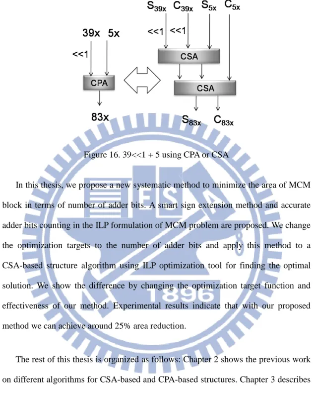
We can bypass the input and 2-bit left shifted input to the output directly. Besides, in a CSA-based structure, the summation of two constants (neither being 1) has 4 inputs. Two adders are needed as shown in Figure 16 since a CSA only has three inputs. This is why a direct transform from CPA structure to CSA structure is not an optimum solution in terms of number of CSA's. So the algorithm using the CSA structure should be developed.

14

Figure 16. 39<<1 + 5 using CPA or CSA

In this thesis, we propose a new systematic method to minimize the area of MCM block in terms of number of adder bits. A smart sign extension method and accurate adder bits counting in the ILP formulation of MCM problem are proposed. We change the optimization targets to the number of adder bits and apply this method to a CSA-based structure algorithm using ILP optimization tool for finding the optimal solution. We show the difference by changing the optimization target function and effectiveness of our method. Experimental results indicate that with our proposed method we can achieve around 25% area reduction.

The rest of this thesis is organized as follows: Chapter 2 shows the previous work on different algorithms for CSA-based and CPA-based structures. Chapter 3 describes the proposed algorithm for area optimization using CSA-based structure. Experimental results are listed in Chapter 4. Chapter 5 is the conclusion.

15

Chapter 2. Previous Work

2.1 CPA-Based Algorithms

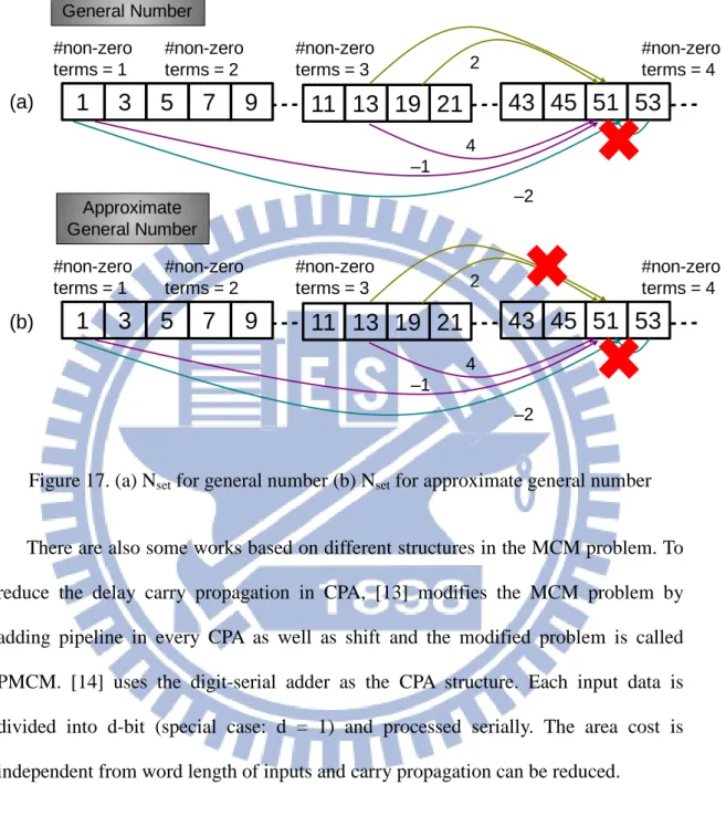
MCM problem has attracted a lot of attention in decades. Many of the proposed algorithms use CPA-based structure. Some of them are CSE algorithms, like [6]–[10]. They may use CSD ([6]–[8]) or MSD ([9] [10]) representation. Others are graph algorithms, like [3]–[5], [11] [12]. [11] is known as RAG-n. It has an optimal part and a heuristic part. In the optimal part, all target constants can be implemented by only one addition is synthesized. In the heuristic part, it relies on a look-up table for single constant optimization. So it lacks sharing of intermediate addition results among different constants. [12] is called Hcub, which includes the same optimal part but is not restricted to a look-up table so it can deal with larger case that RAG-n is not able to handle. [4], [5] use the graph search method BFS or DFS and branch and bound to restrict the search space. An algorithm called general number (GN) [3] uses the same ILP optimization modeling in [6]. But first it would construct a set called Nset which is a result of sorting all positive and odd constants can be expressed using

the given word length(e.g., if word length = 12, sort 1~2047) based on the number of non-zero terms in CSD in ascending order. Then during the decomposition for searching the candidates of additions for a constant, it only considers additions in which both inputs have smaller indices than the index of the constant. An example is shown in Figure 17(a). Assume there are 3 additions that can synthesize 51x: 13x<<2 − x, 19x<<2 + 13x and 53x − x<<1. Since the index of 53 is larger than 51, it will not

16 be a candidate for implementing 51x.

Figure 17. (a) Nset for general number (b) Nset for approximate general number

There are also some works based on different structures in the MCM problem. To reduce the delay carry propagation in CPA, [13] modifies the MCM problem by adding pipeline in every CPA as well as shift and the modified problem is called PMCM. [14] uses the digit-serial adder as the CPA structure. Each input data is divided into d-bit (special case: d = 1) and processed serially. The area cost is independent from word length of inputs and carry propagation can be reduced.

2.2 CSA-Based Algorithms

For high speed DSP application, CSA can be widely used [15]. Using CSA in FIR filter is proposed in [16]. It also shows that using CSA can reduce power consumption.

1

3

5

7

9

11

13

19

21

43

45

51

53

–1 4 2 –2 General Number Approximate General Number #non-zero terms = 2 #non-zero terms = 1 #non-zero terms = 4 #non-zero terms = 3

1

3

5

7

9

11

13

19

21

43

45

51

53

–1 4 2 –2 #non-zero terms = 2 #non-zero terms = 1 #non-zero terms = 4 #non-zero terms = 3 (a) (b)

17

In MCM problem, the direct transform from CPA to CSA of a CPA-based solution is proved that it is not optimal solution in [17]. So the CSA-based algorithm should be developed. A CSE heuristic algorithm is proposed in [18]. It iteratively extracts all three-term subexpressions of constants and then finds the most common one for adder sharing. [19]–[20] are graph algorithms. [19] has an optimal part and a heuristic part. Constants that can be implemented by one adder is synthesized in the optimal part while in heuristic part the unimplemented constants will be implemented either by two CSA's or a corresponding mapping from [17]. [17] has a look-up table of all possible additions can be achieved by up to 5 adders and exhaustive search for area minimization in terms of the number of CSA's is applied. The extra look-up table in [20] is used if the input of the filter is the output of another filter, i.e., the filter input is in the form of sum and carry of a CSA. An exact CSE algorithm and a revised general number algorithm called approximate general number (AGN) are proposed in [21] and transformed into a 0-1 ILP problem as the ILP structure used in [6]. The difference between AGN and GN is that in AGN one input of each CSA must be 1 as illustrated in Figure 18. An example is shown in Figure 17(b). Assume there are 3 additions that can synthesize 51x: 13x<<2 − x, 19x<<2 + 13x and 53x − x<<1. Except for 53 with larger index, the combination of 19 and 13 won't be accepted since neither of them is 1.

Figure 18. One input of each CSA must be 1 C S A C S A x

_–

C S A S_13x C_13x <<2 <<2 C_51x S_51x C_51x S_51x C_13x S_13x C_19x S_19x <<1 <<1

18

Chapter 3. Proposed Algorithm

3.1 Bit Level Area Optimization Using CSA-Based

Structure

Several algorithms of CSA-based MCM optimization are already proposed. However they only count on the number of CSAs, neglecting the size difference of them. The fact that the word length of different CSAs are not identical makes these algorithms not obtaining minimum cost in bit-accuracy. An example is shown in Figure 19. The input is denoted by x and there are two solutions for implementing 51x: 13x<<2 − x and x<<6 − 13x. The constant 13x is implemented by 16x − 4x + x. Implemented by our later proposed method the number of adder bits of 13x<<2 − x is 13 and x<<6 − 13x is 10 if we assume input's word length is 12. ΔAdder bit(%) is (13 − 10) / 13 =23.08 %. Thus only considering number of adder without considering the bit-level accuracy cannot obtain the smaller cost in this case.

Figure 19. Two different additions for implementing 51x have different the number of adder bits

19

However, the word length calculation of CSA involves the number system. Two's complement is the most generally used binary signed number system in digital systems. For a N-bit number A, the MSB A[N − 1] is the sign bit and it represents a negative value –A[N – 1]2(N – 1). On the other hand, the remaining bit A[x] represents the positive value A[x]2x, 𝑥 ∈ {0,1, … , 𝑁 − 2}. The corresponding value of the two's complement is 2 N 1 0 [N 1]2 [ ]2 N i i A A i − − = − − +

∑

For example, if A is an 8-bit two's complement number, the bit A[7] represents the value −A[7]27. The corresponding value is –A[7]*27 + A[6]*26 + … + A[0]*20.

Figure 20. An 8-bit two's complement number

In our proposed algorithm we will mark the sign bit by red square as in Figure 21 because it is different from the other bits. Due to the fact that the positions of sign bit in all three inputs may be different, we may face the problem of adding sign bit with unsigned bits. If we add sign bits with unsigned bits directly, the result will also contain sign bits. However, inserting a sign bit in the middle of a data word is not allowed in 2’s complement number system.

20

Figure 21. MSB is a sign bit while the other bits are unsigned bits

To deal with this problem, the inputs with smaller positions of MSB are needed to do the sign extension. Extend the two inputs with smaller positions of MSB is a trivial way to deal with the problem, but it comes with a high cost in terms of adder bits. An example is shown in Figure 22(a). Assume the inputs 1 and 2 of the addition 16 + 2 + 1 =19 do the trivial sign extension and word length of input variable is 4. The total number of adder bits is 4. But in our proposed method we adjust the sign extension as shown in Figure 22(b). Fewer bits are extended and the number of adder bits for the addition is less. The principle and detail of the algorithm will be discussed in this chapter.

21

Figure 22. (a) Trivial sign extension (b) Smart sign extension

22

3.2 Problem Formulation

As mentioned in 3.1, we have changed the optimization target from reduction of the number of CSA's to reduction of the number of adder bits for implementing all constants. The problem formulation is shown as below:

Area optimization of CSA-based MCM block Problem: Given a set of constants (positive and odd), find the minimum the number of adder bits for implementation of all constant multiplications.

Definition 1: A CSA-based MCM block has single input and multiple output ports that each output port has two data words (sum and carry of a CSA).

Definition 2: Adder bit is a bit which needs a full adder implementation in CSA. The addition in adder bit is not replaced by simpler hardware like wiring and inverter.

3.3 Overall Flow

The overall flow of our proposed algorithm is shown in Figure 23. After the preprocessing of making the given set of constants positive and odd, the following four steps will be executed:

23 1. Find AGN representations for constants

2. Build Boolean network for adder sharing

3. Calculate the number of adder bits for each adder

4. Formulation of 0-1 ILP problem

In step 1, the AGN representations for constants are found. Then in step 2, the connections between constants and additions are built and a Boolean network is constructed to represent the connections. After step 2, the calculation of number of adder bits for each adder is performed in step 3. In step 4, the ILP constraints and optimization target function are transformed from the Boolean network generated in step 2 and calculated adder bits in step 3. Finally the ILP tool (in this thesis, Gurobi_5.0 is used) can be executed to find the optimal solution under the constraints in step 4. ILP-optimized solution is the additions that total number of adder bits is minimal. The details of all 4 steps will be discussed in 3.4~3.7.

24

Input: a set of constants

Make all constants positive and odd

1. Find AGN representations for constants 2. Build Boolean network for adder sharing

3. Calculate #adder bits for each adder

4. Formulation of 0-1 ILP problem

Output: additions that corresponding #adder bit is minimized

Run ILP tool Gurobi_5.0 for optimal solution

25

3.4 Find AGN representations for Constants

To avoid the exponentially increasing number of ILP constraints because the graph algorithms have an extremely large solution space, it is necessary to choose the candidates of additions carefully. We adopt the approximate general number in this step because it provides better solutions than CSE algorithms without adding too many extra constraints. Furthermore, it utilizes the characteristic that adding 1 to a CSA output only needs one CSA as shown in section 2.2. Compared to all previous works, it provides the minimum number of adders to the best of our knowledge.

For a target constant, we first find all combinations of adding or subtracting 2N to another constant (can be negative). For example, 51 = 1<<3 + 43 means the target constant 51 can be implemented by adding 1<<3 = 23 to constant 43. But there is an extra rule mentioned in 2.1. A set called Nset is built and stored in the ascending order

based on the sorting result of all odd constants that can be represented in a given word length with their number of non-zero terms in CSD representation. According to the sorted order in Nset, only the constants with the smaller indices compared to the target

constant is allowed (see Figure 17(b)). An example is showed in Figure 24. Suppose the 51 is the needed constant and the word length of the constant is 7, there are 14 possible candidates of AGN representations. But among these 14 candidates, three of them (−1<<1 + 53, −1<<5 + 83 and −1<<6 + 115) have inputs with larger indices compared to 51. So they won't be the legitimate AGN representations for generating 51x. Furthermore, there are 2 candidates with the same input constant but different shift and sign (1<<6 − 13 and −1 + 13<<2). If only counting number of adder as in [21], they have the same cost and one of them will be removed for reducing ILP

26

constraints. But in our work the number of adder bits of these two adders and corresponding position of MSB and LSB of sum and carry may be different, it is necessary for us to keep all of the candidates.

Figure 24. Legitimate AGN representations of 51

The overall process of finding legal AGN representations for all constants is shown in Table 3. First a set of constant C is inserted of all target constants and the word length of constant is assumed as n . For each element ck in C, it adds or subtracts a left shift (from 0 to n – 1) of 1 and the addition/subtraction results are saved in a temporary set temp_C. For every element in temp_C, it is transformed into a positive and odd constant, c3, and its corresponding AGN representation, o1: ck = s1 * (c3<<m) + s2 * (1<<n), is found. Both s1 and s2 is 1 or – 1 and m as well as n are how many bits should c3 and 1 to be shifted, respectively. If (1) the index of c3 in Nset

is smaller than the index of ck in Nset , (2) o1 is not found before and (3) the number of

non-zero digits of c3 in CSD representation is greater than or equal to 3, o1 will be saved. If the number of non-zero digits of c3 in CSD representation is greater than 3, it will be inserted into C. Finally, ck is removed from C and temp_C is set as an empty set. The process will be executed until C is an empty set.

Ignore one of Implementation in previous work while we have to keep both since their #adder bits are not the same

27

3.5 Construct Boolean Network

If all AGN representations of each constant are found, a Boolean network would be built to represent the connections of all constants and additions. First, we transform all AGN representations to an AND gate. For example, 51 = −1 + 13<<2 is shown in Figure 24. In Figure 25, every edge is either a constant or an adder output. Edge vX Table 3. Overall process of finding legal AGN representations for all constants

28

represents the constant X and edge vX_i represents the ith AGN representation of constant X. Bold edge represents the sum and carry of an addition and thin edge represents the input variable. Each edge has a corresponding binary variable. The value of the binary variable represents whether we need the constants or addition implementation.

Figure 25. Corresponding AND gate of −1 + 13<<2

After AGN representations are transformed into the AND gates, all of the candidates for the same constants are connected to an OR gate as shown in Figure 26. Only part of AGN representations are shown in Figure 26, but in practice all of the AGN representations should be connected to the same OR gate. The output of the OR gate is vX and the meaning of the OR gate is that if we need constant X, at least one of the additions should be implemented.

29

Figure 26. OR gate connected with all AGN representations for 51

The edges v13, v47 and v67 in Figure 26 are not only connected to one AND gate, of course. The sharing for the same input of different additions is common because the sharing is the key of the area minimization in MCM designs. Part of the sharing is shown in Figure 27. If v13 is not only used in −1 + 13<<2 but also in 1<<6 + 13, the branch of edge v13 will appear.

30

Figure 27. Part of the whole Boolean network

3.6 Calculation of Number of Adder Bits for All

Additions

3.6.1 Calculation of Number of Adder Bits

Unlike processor-based design, ASIC designs have the flexibility to adjust the position of MSB (most significant bits) and LSB (least significant bits) according to the dynamic range and resolution of a data word. In MCM design, because of bit-wise shifting, the bit position of every data word may be varied. In our work, calculation of number of adder bits depends on the bit positions of the data words and how we do

31

sign extension. The MSB's and LSB's of the three inputs determine the number of adder bits of an addition. LSB determines the starting point and MSB determines the end point of a series of the full adders in CSA. Besides knowing the adder bits in a CSA, in order to supply the MSB and LSB information to the fanout CSA, the position of the MSB and LSB of both output words (sum and carry) in current CSA would be the information we must know. So when we need to calculate the adder bits of all additions, the MSB and LSB of three inputs of a CSA and its MSB and LSB of both sum and carry are necessary. The properties of input of MCM block such as word length and number system will also affect the calculation. We assume input variable of the MCM block is under the 2's complement representation and the word length of MCM input is equal to the word length of constant.

In our proposed algorithm, the calculation of adder bits of all additions is actually finding the weighting of all AND gates in the Boolean network. An example is shown in Figure 28. First we define MSB(x) is the MSB position of x and LSB(x) is the LSB position of x. Assume MSB’s and LSB’s of sum and carry of v67 are known. In the figure we denote the position of MSB and LSB of sum add carry by ( [MSB(sum):LSB(sum)], [MSB(carry):LSB(carry)] ). And the positions of MSB’s as well as LSB’s of sum and carry of the output edge v51_3 are solved by the smart sign extension method we proposed (will be shown in next section). The number of adder bits in the addition is solved at the same time. Then the positions of MSB's and LSB's of sum and carry of v51_1~v51_n and calculation of number of adder bits for each addition implemented 51 are determined. How we obtain the bit information of v51 after the OR gate will be described in section 3.6.3.

32

Figure 28. Calculation of #adder bits of v51_3

3.6.2

Smart Sign Extension

The smart sign extension we propose is a systematic method to do sign extension for any input condition. The concept is similar to some booth multiplier, however, the booth multiplier is a regular structure and there is no systematic method proposed yet to the best of our knowledge. There are three cases are sorted out according to the inputs of the CSA. We sorted out all input combinations into three cases, with some common parts and some varied parts. We divide this method to two steps due to these three cases. The common first step is for the LSB handling. The second step handles sign extension for each case. Compared with the trivial sign extension, it has less number of adder bits.

First step:

33

MSB such that MSB(z)>= MSB(y) >= MSB(x). For input x, we extend its sign bit to Figure 29. (a) Sign extension for input x (b) Direct wiring (c) First step complete

34

MSB(y) as shown in Figure 29(a). Then for those inputs whose LSB position it's not the largest, we can do direct wiring to the sum and carry. Because there are two outputs and inputs, no full adder is needed. This means from the bit 0 to max(LSB(x), LSB(y), LSB(z)) − 1, no full adder is needed. The starting point of the series of full adders is max(LSB(x), LSB(y), LSB(z)). In Figure 29(b), the LSB positions of input x and input y are not the largest. So for the bits below LSB(z) (i.e., 0~LSB(z) − 1), no full adder is needed. In implementation, the input with the smallest position of LSB will be wired to the sum and the other input will be wired to carry because we want to balance the word length of carry and sum. The smallest position of LSB is 0 since we only implement the odd constant. The position of LSB of sum and carry become 0 and median(LSB(x), LSB(y), LSB(z) ), respectively. The following procedures of proposed algorithm will depend on the largest position of MSB. In Figure 29(c), it is the MSB(z). We find there are three cases would generate different results and should be discussed separately.

Second step:

We will divide this step into 3 cases according to the relative position of MSB(z) and MSB(y). Case 1 is MSB(z) > MSB(y) + 1, case 2 is MSB(z) = MSB(y) + 1 and case 3 is MSB(z) = MSB(y). These three cases contained all possibility because MSB(z) ≥ MSB(y) by our definition.

Case 1: MSB(z) > MSB(y) + 1

In this case, as shown in Figure 30, MSB(z) is at least 2 bits higher than MSB(y). The example used in Figure 30 is a CSA with three inputs and their word lengths are 6. The addition implemented by this CSA is 1<<4 + 1<<2 + 1. So the input x is 1, input

35

y is 1<<2 and input z is 1<<4. The first 4 bits of sum and first 2 bits of carry are from

the first 4 bits of x and first 2 bits of y, respectively. In this case, even if we extend input x to the MSB(y), the bit at MSB(y) in input z is still not sign bit thus can’t be added to x and y directly. So an extra operation is needed. We will inverse the bits at MSB(y) of the input x and y and treat them as the unsigned bits. As shown in Figure 30(b), the equation of this operation is –x5 – y5 = –2 + x5+ y5. The logical value of a

sign bit xs is actually –xs while a inversed Boolean variable xs is denoted by xs , To

prove the equation is a tautology, the truth table of left part and right part of the equation is shown in Table 4.

After handling the sign bit of x and y, we can add these unsigned bits in the middle as shown in Figure 30(c). The end point of the series of the full adders becomes MSB(y) as shown in Figure 30(d). So in this case the number of adder bits of the addition is MSB(y) − max(LSB(x), LSB(y), LSB(z) ) + 1. In this example, the number of adder bits is 7 − 4 + 1 = 4. The bits s4~s7 in sum are the sum outputs and

c3~c6 in carry are the carry outputs of the series of full adders. The bit c2 in carry is

Table 4. The truth table of –x5– y5 and –2 + x5+ y5.

x5 y5 –x5 – y5 –2 + x5+ y5

0 0 –0–0 = 0 −2+1+1=0

0 1 –0–1 = –1 −2+1+0=–1

1 0 –1–0 = –1 −2+0+1=–1

36

actually 0, but we will treat it as a variable to make the carry to be a continuous vector for the simplicity of the whole process.

The −1 at MSB(y) + 1 can be used to transform the bit of input z at the same position from unsigned bit to sign bit. In this example, the equation is -z4. = -1 +z4 .

The truth table of left part and right part of the equation is shown in Table 5 to prove the equation is also a tautology. The inversed z4 can be used as the sign bit of the sum

and the remaining bit in the input z (i.e., the sign bit z6) can be wired to the carry. So

both sum and carry are in the format of two's complement. The Table 6 shows the MSB and LSB of both sum and carry.

Table 6. The MSB and LSB of both sum and carry in case 1

MSB LSB

Sum MSB(y) +1 0

Carry MSB(z) median(LSB(x), LSB(y), LSB(z) ) Table 5. The truth table of –1 +z4 and –z4

z4 –1 +z4 –z4

0 –1+0 = –1 –1

37

Figure 30. Example of case 1 after sign extension

Case 2: MSB(z) = MSB(y) + 1

In this case, as shown in Figure 31, MSB(z) is at actually 1 bit higher than MSB(y). The example used in Figure 31 is a CSA with three inputs is a CSA with three inputs and their word lengths are 6. The addition implemented by this CSA is 1<<3 + 1<<2 + 1. So the input x is 1, input y is 1<<2 and input z is 1<<3. The first 3 bits of sum and

38

first 1 bit of carry are from the first 3 bits of x and first 1 bits of y, respectively.

The following procedure is very similar to the procedure in case 1. We will inverse the bits at MSB(y) of the input x and y and treat them as the unsigned bits. This operation will increase an extra −1 at MSB(y) + 1. In Figure 31(b), this means –x5 – y5 = –2 + x5+ y5. After adding the middle bits, the bits s3~s7 in sum are the sum

outputs and c2~c6 in carry are the carry outputs as shown in Figure 31(d). The number

of adder bits is also MSB(y) − max(LSB(x), LSB(y), LSB(z) ) + 1. In the example used in Figure 31, it is 7 − 3 + 1 = 5. The bit c1 in carry is actually 0, but we will treat

it as a variable like in case 1.

The different point is the bit at MSB(y) + 1 of input z is the sign bit of the input z. In this example as shown in Figure 31(d), it is −1 − z5, not −1 + z5 in case 1. We will

do 1-bit sign extension for input z and inverse the bit at MSB(y) +1 of input z. The inversed bit is used as the sign bit of sum and the extended bit is used as the sign bit of carry. In the example, the sign bit of sum is z5 and the sign bit of carry is z5. This

operation is actually the equation –1 – z5= –1 + z5-2z5 = – z5 -2z5 . Then we can take

z5 as the sign bit of sum and take z5 as sign bit of carry. The Table 7 shows the MSB

and LSB of both sum and carry.

Table 7. The MSB and LSB of both sum and carry in case 2

MSB LSB

Sum MSB(y) +1 0

39

Figure 31. Example of case 2 after sign extension

Case 3: MSB(z) = MSB(y)

In this case, as shown in Figure 32, MSB(z) equals MSB(y). The example used in Figure 32 is a CSA with three inputs and their word lengths are 6. The addition implemented by this CSA is 1<<2 + 1<<2 + 1. So the input x is 1, input y is 1<<2 and input z is 1<<2. The first 2 bits of sum are from the first 2 bits of x. In this example,

40

due to LSB(y) = LSB(z), no bit is wired from input y or input z to the carry.

Since the bits at MSB(y) of three inputs are all sign bits, no extra operation is needed to add these three bits. The following equation −x5− y5− z5 = − (x5 + y5 + z5)

= −(sum + carry) = −sum −carry shows why no extra operation is needed. The sum and carry of the full adder can be used as the sign bit of sum and carry of CSA, respectively. The bits s2~s7 in sum are the sum outputs and c0~c6 in carry are the carry

outputs of the series of full adders. The number of adder bits is also MSB(y) − max(LSB(x), LSB(y), LSB(z) ) + 1. In the example used in Figure 32, it is 7 − 2 + 1 = 6. The bit c0 in carry is actually 0, but we will treat it as a variable like in case 1. The

Table 8 shows the MSB and LSB of both sum and carry.

Table 9 shows the equations of the position of MSB and LSB of sum and carry as well as the number of adder bits for all three cases. We can find the equations of the number of adder bits are the same for all three cases. And the equations of the position of LSB of both sum and carry is the same for all three cases, too. Only the equations of the position of MSB of sum and carry are slightly different for the 3 cases. By using these equations, we can calculate the required number of adder bits and the bit positions of the outputs if input bit information is available.

Table 8. The MSB and LSB of both sum and carry in case 3

MSB LSB

Sum MSB(y) 0

41

Table 9. MSB and LSB of sum and carry as well as the number of adder bits for all three cases

MSB(sum) LSB(sum) MSB(carry) LSB(carry)

#adder bits

MSB(z)> MSB(y) +1

MSB(y) +1 0 MSB(z) median(LSB(x), LSB(y) , LSB(z) )

MSB(y)- max(LSB(x), LSB(y) , LSB(z) )+ 1

MSB(z) = MSB(y) +1

MSB(y) +1 0 MSB(z) +1 median(LSB(x), LSB(y) , LSB(z) )

MSB(y)- max(LSB(x), LSB(y) , LSB(z) ) + 1

MSB(z) = MSB(y)

MSB(y) 0 MSB(z) +1 median(LSB(x), LSB(y) , LSB(z) )

MSB(y) - max(LSB(x), LSB(y) , LSB(z) ) + 1

Figure 32. Example of case 3 after sign extension

42

3.6.3 Bit Propagation for OR Operation

Figure 33 shows an example why we need to discuss the OR gate. Assume the word length of input variable of MCM block is 12. After we find the number of adder bits as well as the positions of MSB and LSB of sum and carry of additions v51_1 and

v51_2, we can see that the position of their MSB of sum and carry are not equal. The

MSB(sum) of v51_1 is 17 and the MSB(sum) of v51_2 is 16 and the MSB(carry) of

v51_1 is 18 and the MSB(carry) of v51_2 is 17. The output information of all inputs

of OR gate are not the same for every cases, so some decision must be made such that we can calculated the additions with at least one input is 51.

Figure 33.Example of Bit Propagation for OR operation

The exact solution of this problem can be found if setting the number of MSB of OR gate in the form of the following equation:

_ * MSB( _ )

i

vX i vX i

∑

But this will turn the optimization from ILP to quadratic programming (multiplying two variable makes the constraint quadratic), which will cause runtime

51([?:?], [?:?]) 13 ([14:0], [15:2]) 1 [11:0] 67 ([14:0], [17:2]) 1[11:0] 51_2 ([16:0], [17:2]) 51_1([17:0], [18:2]) <<4 – <<2 – 1[11:0] <<8 307_1([?:?], [?:?]) 307([?:?], [?:?]) 13 12

43

explosion. Since this exact solution is not appropriate, we decise to make estimation instead.

Our strategy is taking the average of MSB of all inputs of OR gate and round down the average to the nearest whole digit (flooring of the average).

1 1 1 1 MSB( ) sum : MSB( _ _ ) , carry : MSB( _ _ ) N N i i vX vX i sum vX i carry N = N =     = _{   } 

∑

 

∑

 1 1 1 1 LSB( ) sum : LSB( _ _ ) , carry : LSB( _ _ ) N N i i vX vX i sum vX i carry N = N =     = _{   } 

∑

 

∑



where N is the number of candidate additions and vX_i_sum is the sum and

vX_i_carry is the carry of vX_i. Quantization to integer is necessary for our proposed

method to calculate bit positions. We adopted floor function instead of rounding because the ILP optimization will potentially select smaller word length solution thus the result is usually slightly smaller than average and selecting floor function of average can reduce the estimation error.

3.7 Transform Boolean Network to 0-1 ILP Problem

After the number of adder bits of each addition is determined, the Boolean network can be transformed to ILP problem. ILP problem is finding a solution to maximize the target function under the given linear constraints with some variable limited to integers. An ILP problem can be written as:

44 Maximize: cTx

Subject to: Ax <= b , x>=0, and x ∈ z

The vector c is the vector of coefficients of target function, vector x is the variable vector. Matrix A and vector b are used to describe the constraints.

An example is shown in Figure 34. For the variables vX represent the target constants, they will be set as 1 such that these variables must be implemented. Like

v51 in the Figure 34, the constraint of v51 = 1 is set. For each variable vX represent

the output of OR gate, a constraint is set in the form of:

1 _ X N i vX i vX = >=

∑

where NX is the number of inputs of the OR gate. This kind of constraints is to make sure if vX is required, at least one of the candidate additions of vX is implemented. For each variable vX_i represents the output of AND gate, a constraint is set in the form of:

_ min( , )

vX i<= vY vZ

where vY and vZ are the inputs of the AND gate. This constraint is set to make sure if

vX_i is needed to be implemented, its inputs vY and vZ have to be implemented at the

same time. But in AGN algorithm one of the inputs is always 1 while the other is a constant. Thus, one of the inputs is always true. Using this constraint mainly for keeping flexibility for using not only AGN in our experiments. Finally, the optimization target function is set in the form of:

45 1 minimize _ * _ X N X T i vX i wX i ∈ =

∑ ∑

where T is the target constant set, NX is the number of candidate additions of constant X and wX_i is the weighting(i.e., the number of adder bits) of the addition vX_i. So the total number of adder bits can be minimized.

Figure 34. Boolean network with weighting in terms of number of adder bits

After all of the above procedures, we can run the ILP tool for finding the optimum solution in terms of adder bits. After the optimum solution is found, we can obtained a result of total adder bits from ILP tool, but this value is not a real value because the cost function in ILP is an estimated value. In our algorithm we apply the same techniques of bit calculation for the resultant MCM block to get a real cost result.

v51

v13

v47

v67

1

1

1

v51_1

v51_2

v51_3

<<2

–

–

1

1

v77

v323

<<6 <<2 <<4 <<8

10

13

13

12

10

v77_1

v323_1

46

Chapter 4. Experimental Results

We implement our proposed algorithm by C++ and Gurobi_5.0 is used for our ILP optimization. We run the compiled executable binary file on the work station with the following specification:

• OS: CentOS 5.9 (final) 2.6.18-194.17.4.el5

• CPU: Intel Xeon QC E5620 2.4GHz

• RAM: 4GB*18, DDR3-1333

There are two experiments in this thesis. One of them is the implementation of 10 FIR filter benchmarks while the other is the implementation of uniformly distributed random constants. In both experiments we assume the word length of input variable equals the word length of the constant.

In the first experiment, we use 10 digital FIR filters benchmarks. The first 5 FIR filters are cited from [22], while the rest of them are cited from [23] and their original reference are [24]–[28]. Table 10 is the definition of different techniques. We set the result of using trivial sign extension and optimizing the number of adders as the reference point. Table 11 list 10 filters we used.

47

We show the comparison in terms of number of adder bits between trivial sign extension and smart sign extension with optimizing the number of adders in Table 12. The improvement is range from 13.4% to 26.1% and 17.8% in average. It is proved

Table 11. 10 FIR filters used in Exp.1

FIR FIR name in website Original

reference [19] FIR1 fir3 FIR2 fir7 FIR3 fir12 FIR4 fir22 FIR5 fir23 [20] FIR6 JOHANSSON08_30 [21] FIR7 LIMAKT08_121 [22] FIR8 VINOD03_26B [23] FIR9 YOSHINO90_64 [24] FIR10 LIM83_121 [25]

Table 10. Definition of different techniques

Trivial sign

extension

Smart sign extension Optimization target:

#adders Ref. (a)

Optimization target:

48

that our proposed algorithm can reduce the number of adder bits effectively.

If we want more improvement, changing the optimization targets from number of adders to number of adder bits is considered. In the Table 13, the comparison of changing the optimization target with full sign extension is shown. The improvement is 8.2% and estimation error is 0.8% in average. The number of addition is slightly increased because changing the optimization targets from number of adders to number of adder bits may increase number of adder in some special cases. However, actually for each bit in a CSA there is no connection to any other bits in this CSA. It is natural that in automatic placement and routing (APR) stage of the AISC design flow, the adder hierarchy will be flattened to obtain better wiring reduction. Thus the extra number of adder will not cause any problem in our point of view.

Table 12. Comparison between Ref. and (a)

FIR 1 FIR 2 FIR 3 FIR 4 FIR 5 FIR 6 FIR 7 FIR 8 FIR 9 FIR 10 Avg.

WL. 12 14 18 16 14 10 14 14 13 14 #taps 40 60 120 300 40 30 121 26 64 121 Ref. #adders 15 34 96 81 29 28 39 23 20 58 #adder bits 207 554 2231 1493 500 337 637 422 301 957 Run time(s) 0.34 1.7 171.9 3.3 2.4 0.17 2.6 6.3 0.18 8.7 (a) #adders 15 34 96 81 29 28 39 23 20 58 #adder bits 162 463 1932 1255 430 249 536 346 243 793 Δadder bits(%) 21.7 16.4 13.4 15.9 14.0 26.1 15.9 18.0 19.3 17.1 17.8 Run time(s) 0.35 1.6 172.7 3.2 2.4 0.18 2.6 6.3 0.17 8.7

49

Then we change the optimization target with our proposed method and compare the result with optimizing number of adders with full sign extension. The result is shown in Table 14. We can discover that the improvement is now 25.6% in average and it is roughly the summation of the improvements shown in Table 10 and Table 11. The two techniques does not disturb each other to much so changing the optimization target to number of adder bits with our method is the best way to get more

Table 13. Comparison between Ref. and (b)

FIR 1 FIR 2 FIR 3 FIR 4 FIR 5 FIR 6 FIR 7 FIR 8 FIR 9 FIR 10 Avg.

WL. 12 14 18 16 14 10 14 14 13 14 #taps 40 60 120 300 40 30 121 26 64 121 Ref. #adders 15 34 96 81 29 28 39 23 20 58 #adder bits 207 554 2231 1493 500 337 637 422 301 957 Run time(s) 0.34 1.7 171.9 3.3 2.4 0.17 2.6 6.3 0.18 8.7 (b) #adders 15 35 99 81 29 28 39 23 20 59 #adder bits 192 510 2050 1347 460 309 580 379 282 885 Δadders (%) 0.0 -2.9 -3.1 0.0 0.0 0.0 0.0 0.0 0.0 -1.7 -0.8 Δadder bits(%) 7.2 7.9 8.1 9.8 8.0 8.3 8.9 10.2 6.3 7.5 8.2 #adder bits (Est.) 193 508 2002 1351 454 309 581 373 283 876 |Error| (%) 0.5 0.4 2.3 0.3 1.3 0.0 0.2 1.6 0.4 1.0 0.8 Run time(s) 0.37 1.7 291.4 3.4 2.9 0.17 3.1 6.9 0.17 11.7

50 improvement in terms of adder bits.

In the second experiment, we use different sets of uniform random constants. We generate 100 sets of constants of different word length and different numbers of constants in the set and report the average improvement of 100 sets of constants. All results of (a), (b), and (a) + (b) are compared to the results of Ref. The area improvement of (a) decreases if bit width of constants increases. On the other hand, the area improvement of (b) increases slightly as the number of constants increases. The effect of (a) is more obvious in the area improvement of (a) + (b).

Table 14. Comparison between Ref. and (a) + (b)

FIR 1 FIR 2 FIR 3 FIR 4 FIR 5 FIR 6 FIR 7 FIR 8 FIR 9 FIR 10 Avg.

WL. 12 14 18 16 14 10 14 14 13 14 #taps 40 60 120 300 40 30 121 26 64 121 Ref. #adders 15 34 96 81 29 28 39 23 20 58 #adder bits 207 554 2231 1493 500 337 637 422 301 957 Run time(s) 0.34 1.7 171.9 3.3 2.4 0.17 2.6 6.3 0.18 8.7 (a)+(b) #adders 15 35 100 81 29 28 41 23 20 61 #adder bits 151 425 1737 1105 386 225 478 307 228 716 Δadders (%) 0.0 -2.9 -4.2 0.0 0.0 0.0 -5.1 0.0 0.0 -5.2 -1.7 Δadder bits (%) 27.1 23.3 22.1 26.0 22.8 33.2 25.0 27.3 24.3 25.2 25.6 #adder bits (Est.) 152 422 1727 1113 375 226 478 297 229 717 |Error| (%) 0.7 0.7 0.6 0.7 2.8 0.4 0.0 3.3 0.4 0.1 1.0 Run time(s) 0.35 2.3 1169.8 3.4 2.8 0.18 2.9 7.8 0.17 10.4

51

Table 15. Exp. 2 results for different word length and #constants

#const. 20 40 60

WL. 10 12 14 10 12 14 10 12 14

(a) ΔAdder bit (%) 23.1 18.4 16.6 22.4 18.6 16.0 22.5 18.1 15.6

(b) ΔAdder (%) -1.3 -3.0 -4.3 -1.2 -3.0 -4.3 -0.8 -3.5 -4.4 ΔAdder bit (%) 7.6 8.7 8.7 9.8 9.5 9.2 11.3 10.0 9.3 |Error| (%) 0.7 0.9 0.9 0.7 0.9 1.6 0.6 0.9 1.6 (a)+(b) ΔAdder (%) -3.6 -5.3 -6.7 -3.0 -6.0 -7.3 -2.6 -6.6 -7.6 ΔAdder bit (%) 31.0 28.0 25.9 32.1 28.8 26.1 33.4 28.8 26.0 |Error| (%) 0.5 0.8 0.8 0.5 0.8 0.8 0.4 0.6 0.8

52

Chapter 5. Conclusion

In this thesis, we propose a systematic method for area optimization of carry-save-adder-based multiple constant multiplication designs. A smart sign extension method is proposed and combined with the accurate bit counting in the ILP formulation of MCM problem. By using this systematic method, the area optimization in terms of adder bits can be further improved. Experimental results show that our new modeling is effective and the combination of our modeling as well as optimizing the number of adder bits can get more area improvement.