國
立
交
通
大
學
資訊科學與工程研究所
博 士 論 文
應用組合對局知識解決遊戲及改良
搜尋效能
Solving Games and Improving Search Performance
with Embedded Combinatorial Game Knowledge
研 究 生:單益章
指導教授:吳毅成 教授
高國元 教授
應用組合對局知識解決遊戲及改良搜尋效能
Solving Games and Improving Search Performance with Embedded
Combinatorial Game Knowledge
研 究 生:單益章
Student:Yi-Chang Shan
指導教授:吳毅成
高國元
Advisor:I-Chen Wu
Kuo-Yuan Kao
國 立 交 通 大 學
資 訊 科 學 與 工 程 研 究 所
博 士 論 文
A DissertationSubmitted to Institute of Computer Science and Engineering College of Computer Science
National Chiao Tung University in partial Fulfillment of the Requirements
for the Degree of Doctor of Philosophy
in
Computer Science
October 2013
Hsinchu, Taiwan, Republic of China
應用組合對局知識解決遊戲及改良搜尋效能
研究生:單益章
指導教授:吳毅成 博士
高國元 博士
國立交通大學資訊科學與工程研究所博士班
摘要
本篇論文,主要是應用組合對局知識解決遊戲及改良搜尋效能。組合對局理論已 經成為許多益智遊戲分析的基本數學模型,其利用數學代數的特性來降低問題的複雜 度 。 本 論 文 主 要 研 究 三 種 組 合 對 局 遊 戲 , 包 括 三 角 殺 棋 (Triangular Nim) 、 XT Domineering 及 NoGo。 首先,三角殺棋是一種 Nim 的變形,是流行台灣及中國的二人遊戲。本論文使用 Retrograde 方法,全解九層三角殺棋盤面,並運用旋轉及對稱方法,降低記憶空間需 求達 5.72 倍,並增進運算速度達 4.62 倍。 第二、本論文介 紹新的組合對 局遊戲 XT Domineering 及其 數學分析, XT Domineering 其變化來自於 Domineering。變化後的規則,在遊戲中所有盤面皆為微數 字(Infinitesimal),計算得出所有 3×3 盤面的遊戲值(Game values),並得出每一盤面的 遊戲值為 8 種基本微數字的線性組合,利用一個簡單代數和的式子,即可以迅速算出 雙方勝敗,以取代搜尋全部遊戲樹(Game tree)。第三、本論文分析 2011 年 BIRS 組合對局會議提出的一種新的組合對局遊戲 NoGo, 計算其許多 4×4 NoGo 盤面的遊戲值,發現其最高溫度(Temperature)為 2,並在研 究中推導出一些基本定理,以幫助我們瞭解 NoGo 遊戲特性。
S
olving Games and Improving Search Performance with Embedded
Combinatorial Game Knowledge
Student:Yi-Chang Shan
Advisor:Dr. I-Chen Wu
Dr. Kuo-Yuan Kao
Institute of Computer Science and Engineering
National Chiao Tung University
Abstract
In this thesis, we study to solve games and improve search performances with embedded combinatorial game knowledge. Combinatorial game theory (CGT) has become the common fundamental mathematical model for the analysis of many intelligent games. CGT uses algebra characteristics to reduce the complexity of many intelligent games. For this study, we investigate three combinatorial games, including Triangular Nim, XT Domineering and NoGo.
First, Triangular Nim, one variant of the game Nim, is a common two-player game in Taiwan and China. Using a retrograde method, we strongly solve nine layer Triangular Nim. In our design, improved by removing some rotated and mirrored positions, the program reduces the memory by a factor of 5.72 and the computation time by a factor of 4.62.
Secondly, we introduce a new combinatorial game, named XT Domineering, together with its mathematical analysis. XT Domineering is modified from the Domineering game with the game value of each position becoming an infinitesimal. We calculate the game values of all 3×3 positions and shows that each 3×3 position’s game value is a linear
combination of 8 elementary infinitesimals. A simple rule is presented to determine the optimal outcome of any sum of these positions, instead of searching the whole game trees.
Thirdly, NoGo is a game introduced by the organizers of the BIRS workshop on Combinatorial Game Theory 2011 for being a completely new combinatorial game. We calculate the game values of many 4×4 NoGo positions and find the maximum of temperature is 2 among them. We also present some propositions to help us understand the characteristics of NoGo game.
致謝
感謝指導老師吳毅成教授及高國元教授多年來的提攜與照顧,不斷地指導及鼓勵 我做研究。二位老師在理論和實務方面的教學研究,指引我研究的方向,我將秉持老 師的教導,在未來的道路上,一步步努力前進。 除了影響我最深的老師之外,特別感謝我的內人,在研究過程中,一直鼓勵、扶 持和砥礪我,讓我無後顧之憂的研究,順利通過這充滿困難、歡欣和淚水的博士道路。 感謝論文口試委員吳昇教授、林順喜教授、許舜欽教授、陳榮傑教授、蔡錫鈞教 授和顏士淨教授(以上按姓氏筆劃排列),對論文的改進方向,提出寶貴的意見,讓 我的研究能更上層樓。 培育了我多年的交大和我在 CYC Lab 的所有好友們,給予我各式各樣的支持, 在此衷心的感謝大家,包括隆彬學長、秉宏學長,博班同學德中、宏軒、汶傑,及學 弟冠翬、益嘉、博玄、挺富、元耀、振綱、庭築、育賢…等等,特別感謝學弟在我的 口試時細心地幫我準備餐點。 最後,感謝從小教導我的爸爸、媽媽及和讓我無後顧之憂的岳父、岳母及所有幫 助我的兄弟姊妹,讓我可以專心在論文研究,讓我在遇到困難時,內心仍能充滿溫暖 向前。沒有您們,這篇論文將無法完成。謹以此論文獻給我敬愛的師長及最摯愛的家 人。 單益章 2013 年 10 月 12 日Contents
摘要 ... i
Abstract... ii
致謝 ... iv
Contents ...v
List of Figures ... vii
List of Tables ... ix
Chapter 1 Introduction ...1
1.1 Background...1
1.2 Game tree search ...2
1.2.1 Min-Max Tree ...2
1.2.2 Monte Carlo Tree Search ...3
1.3 Combinatorial Game Theory ...5
1.4 Framework of Research ...7
1.5 Organization ...8
Chapter 2 Triangular Nim ...9
2.1 Introduction ...9
2.2 Related Work ... 12
2.2.1 Backward Induction Approach ... 12
2.2.2 Retrograde Method ... 14
2.3 Solving Approach ... 15
2.3.1 Data Structures and Algorithms ... 15
2.3.2 Removing Redundancy ... 19
2.4 Experimental results... 22
2.4.1 Eight Layer Triangular Nim ... 22
2.4.2 Nine Layer Triangular Nim ... 25
2.5 Conclusion ... 28
Chapter 3 XT Domineering: A New Combinatorial Game ... 30
3.1 Introduction ... 30
3.2 Combinatorial Games ... 31
3.2.1 Numbers ... 32
3.2.2 Nimbers ... 32
3.2.3 Sumbers ... 33
3.3 Domineering and XT Domineering ... 36
3.4 Game Values of 3×3 XT Domineering... 38
3.5 Outcome of 3×3 XT Domineering ... 43
3.6 Conclusion And Further Consideration ... 46
Chapter 4 NoGo Endgame Analysis ... 48
4.1. Introduction ... 48
4.2. Classification of Moves ... 49
4.3. Mean and Temperature ... 50
4.3.1 Definitions of Mean and Temperature ... 51
4.3.2 Thermograph ... 52
4.4. Game Values of NoGo Positions ... 54
4.4.1 Game Values ... 55
4.4.2 Means and Temperatures ... 58
4.4.3 More Analysis ... 63
4.5. NoGo Propositions ... 64
4.6. Conclusion ... 72
Chapter 5 Conclusions ... 73
References ... 75
Appendix A The Derivations for XT Domineering Games Values of Positions .... 81
Appendix B The proof for XT Domineering inequalities ... 85
List of Figures
Figure 1. An example of minimax Tree. ...2
Figure 2. Monte Carlo Tree Search ...5
Figure 3. The framework of research ...7
Figure 4. A scenario of Triangular Nim with side size five. ... 10
Figure 5. A piece mapping of 5 layer Triangular Nim. ... 13
Figure 6. Six block representations for 8 layer Triangular Nim. ... 16
Figure 7. Inter-block updates of the block representations in Figure 6 (a) and (b), respectively. ... 19
Figure 8. Six rotated and mirrored blocks. ... 20
Figure 9. An isomorphic group with one, two and three distinct blocks only. ... 21
Figure 10. The moves to win in 8 layer normal Triangular Nim. ... 24
Figure 11. The moves to win in 8 layer misère Triangular Nim. ... 24
Figure 12. Three block representations with 13 BID pieces. ... 25
Figure 13. Three block representations with 15 BID pieces. ... 26
Figure 14. The moves to win in 9 layer normal Triangular Nim. ... 27
Figure 15. The moves to win in 9 layer misère Triangular Nim. ... 27
Figure 16. The ratio of the number of P-positions to that of N-positions. ... 28
Figure 17. Middle game of 6×6 Domineering. ... 36
Figure 18. Sub-positions of the graph in Figure 17 ... 37
Figure 19. Some game values in Domineering. ... 37
Figure 20. Some game values in XT Domineering. ... 42
Figure 21. Some game values in XT Domineering. ... 43
Figure 22. Some game values in XT Domineering. ... 46
Figure 23: The classification of moves in NoGo. ... 49
Figure 24: Thermographs of (a) a simple max function and (b) a simple min function. ... 53
Figure 25: The thermograph of 𝐺 = {3|{0| − 2}}. ... 54
Figure 26. A specific 5×5 Nogo position. ... 62
Figure 27. The temperature is greater than 2 in a 4×7 NoGo position. ... 63
Figure 28. The example of NoGo definitions. ... 65
Figure 29. Each No-Go has game value zero... 66
Figure 30. The example of B-Dragons and W-Dragons. ... 67
Figure 32. The board forms left and right independent regions. ... 69 Figure 33. The symbol of black triangle is represented for B-EGo . ... 71 Figure 34. The example of B-Ego and W-Ego. ... 72 Figure 35. Deriving both game values of C and E of Figure 18 in (a) and (b) respectively. .... 81 Figure 36. Deriving the game values of C + E. ... 82 Figure 37. Deriving both game values of C and E of Figure 18 in (a) and (b) respectively. .... 83 Figure 38. Deriving the game values of C + E. ... 84
List of Tables
Table 1. Experimental results for the block representations without removing redundancy in
Figure 6. ... 23
Table 2. Experimental results for three block representations with removing redundancy in Figure 6. ... 24
Table 3. Experimental results for the block representations in Figure 12. ... 25
Table 4. Experimental results for the block representations in Figure 13. ... 26
Table 5. The result of k layer Triangular Nim. ... 28
Table 6. Game values of 3×3 XT Domineering ... 41
Table 7. Minimum ups U required for U + SB + SC > 0 ... 44
Table 8. The list of special game values of 4×4 NoGo. ... 58
Table 9. The highest and lowest of means with endgame search depth 6 and 8 of 4×4 NoGo 59 Table 10. The lists of maximum temperature with endgame search depth 6 in 4×4 NoGo. .... 61
Table 11. The lists of maximum temperature with endgame search depth 8 in 4×4 NoGo. ... 62
Table 12. The temperature analysis with endgame search depth 6 in 4×4 NoGo positions. .... 64
Chapter 1 Introduction
Combinatorial game theory (CGT) [7][20] has become the common fundamental mathematical model for the analysis of many intelligent games. In CGT, a game can be viewed as a tree where the branches are classified into left and right branches and the terminal nodes are numbers. A sum of games is a collection of trees where each player can choose one to move at a turn. Combinatorial games include many games like chess [23][49], Chinese chess [26], Go [6][53], Heap Go [41][42], Nim [8], Triangular Nim [3][14][33][47][57], Domineering [5][9][12][16][17][44], XT domineering [40][43], and NoGo [15][45]. If the positions of games are public to both players and their all available moves are also public, noted perfect information game [2]. Other games are called imperfect
information game, like Bridge Poker, Mahjong [68][69] and so on. These games hide some
information from other players.
1.1 Background
CGT is one of the applied mathematics which uses algebra characteristics to reduce the complexity of many intelligent games. Based on the theory, playing or solving many combinatorial games may simply become mathematical calculations, such as summation, instead of a complex tree search.
CGT studies two-player games with perfect information. The two players are assumed to take turns alternatively, and a game is considered as a sum of local positions, where each player can choose one local position to move at each turn.
1.2 Game tree search
The game search has been an important issue in computer science. From early minimax tree search to recently Monte Carlo Tree Search (MCTS), most of researches focused on improvement of tree search. In the following two subsections, we review minimax search and MCTS, respectively.
1.2.1 Minimax Tree
Figure 1 (below) shows a minimax tree. Square nodes usually represent Max nodes which get the maximum of the values of all children, and circular nodes represent Min nodes which get the minimum of the values of all children. Claude Shannon first estimated lower bound on the game-tree complexity of chess [58]. Recently, MCTS is a search paradigm that has been remarkably successful in computer games like Go. MCTS uses Monte-Carlo simulation to evaluate the values of nodes in a search tree. Currently MCTS is popular for game search method which also follows the original game-tree estimated.
Figure 1. An example of minimax Tree.
max min max min 7 1 5 6 7 2 8 1 7 2 7 8 1
1.2.2 Monte Carlo Tree Search
MCTS [21] is a search paradigm for two-player and zero-sum games. It has been applied to various computer games [4][11][25][29][48][56][61][62][66]. This subsection reviews the basic ideas of MCTS and its related policy improvements, following the definitions of [30].
Let S denote the state space of a game, and st be the state of a game at time t. Let A
denote the space of actions and let A(s) denotes the set of legal actions from state s. The two
players alternate turns, at each turn t selecting an action at in A(st). The game finishes upon
reaching a terminal state with outcome z. One player’s goal is to maximize z; the other player’s goal is to minimize z. A policy π is defined as a stochastic action selection strategy
that determines the probability of selecting actions in any given state. Q( as, ) is defined as
the expected outcome after playing action a in state s, and then following policy π for both players until termination.
Q(s,a)E[z|st s,at a]
The basic idea of MCTS is to evaluate the expected outcome online from simulated
games. Each simulated game starts from a root state s0, and sequentially samples actions until
the game terminates. At each step t of simulation, a simulation policy π is used to select an
action at. The outcome z of each simulated game is used to update the Q-values encountered
during that simulation. This update can be implemented incrementally by incrementing the
state-action simulation count N(st,at)and updating the Q-value towards the outcome z.
( , ) ) , ( -) , ( ) , ( t t t t t t t t a s N a s Q z a s Q a s Q
There are two policy stages in the simulations. A tree policy is used to select actions on
the state st represented in the search tree, while a default policy is used on those not in the
tree, mainly for the playout simulations.
The second idea of MCTS is policy improvement. The values in the search tree are used as references to select the actions during subsequent simulations. As the number of simulations increases, the policy π continues to improve. Eventually, with sufficient simulations, the policy will reach the optimal strategy.
UCT [28] is an example of policy improvement scheme. It selects actions by using the UCB algorithm which maximizes an upper confidence bound on the value of actions. Specifically, the Q-value is augmented by an exploration bonus that is high for rarely visited actions, and the policy selects the action a* maximizing the augmented value.
) s, ( ) ( log ) , ( ) , ( a N s N c a s Q a s QUCB
a*argmaxaQUCB(s,a)
where c is a scalar exploration constant, N(s) is the number of visits to state s, and log is the natural logarithm. The underlying idea of UCT is to provide a balance between exploitation of the current best action and exploration of other potential better actions.
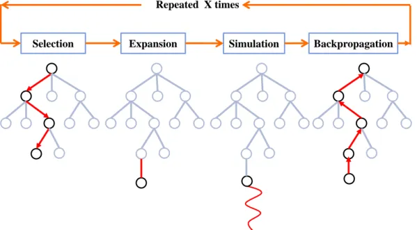
Figure 2. Monte Carlo Tree Search
Figure 2 shows four steps in MCTS including selection, expansion, simulation and back propagation in loop while.
1.3 Combinatorial Game Theory
Combinatorial game theory [7][20] starts from a simple definition of game: A game is an ordered pair of sets of games. Conventionally, a game G is denoted as:
G = {GL | GR},
where GL and GR are sets of games. A special game is named 0, when both GL and GR
are empty sets, .
Negation, addition and comparisons are defined as follows.
GGRGL
G + HGL + H,G+ HLGR + H,G+ HR
Selection Expansion Simulation Backpropagation Repeated X times
G 0, if and only if there is no element in GR 0,
G 0, if and only if G 0,
G H, if and only if G H 0.
When neither G H nor G H, it is said G confused with H, denoted by G || H. G <| H
denotes either G < H or G || H, and similarly for G |> H. Furthermore, an equivalence relation on the sets of games is defined as follows.
G H, if and only if G H and G H.
The equivalence classes of games form an algebraic group, which can be used to describe the positions of many intelligent games as follows.
There are two players (say Left and Right) move alternatively.
The game is a sum of positions; each position has two sets of next positions; one for
each player.
On each player’s turn, the player can choose one position and move the position to one
of its next positions.
The player who cannot find a move is the loser.
For each game G, there are 4 types of possible outcomes. The corresponding relations between G and 0 are described as below:
G 0: The first player cannot win the game.
G < 0: Left cannot win the game.
G > 0: Right cannot win the game.
In general, players are concerned with who can win a given game G. Mathematically speaking, the question is equivalent to determining one of the above four relations between
G and 0.
1.4 Framework of Research
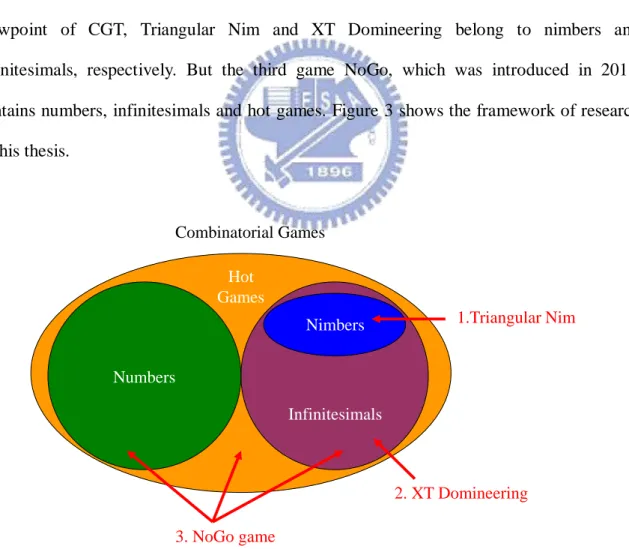
In this thesis, we study to solve games and improve search performances with embedded combinatorial game knowledge. For this study, we investigate three combinatorial games, including Triangular Nim, XT Domineering and NoGo. From the viewpoint of CGT, Triangular Nim and XT Domineering belong to nimbers and infinitesimals, respectively. But the third game NoGo, which was introduced in 2011, contains numbers, infinitesimals and hot games. Figure 3 shows the framework of research in this thesis.
Figure 3. The framework of research Combinatorial Games Numbers Nimbers Infinitesimals 2. XT Domineering 3. NoGo game 1.Triangular Nim Hot Games
1.5 Organization
Chapter 2 presents the solving of nine layer Triangular Nim. We propose some methods to improve the performance, such as designing data structures in blocks, using the retrograde method, removing redundancy and selecting the block representation with the less number of inter-block updates.
Chapter 3 introduces a new game: XT domineering. We present a mathematical approach to solve sums of 3×3 XT Domineering and find several infinitesimal games with interesting properties. Chapter 4 is NoGo game analysis and derives three important
Chapter 2 Triangular Nim
This chapter introduces the game of Triangular Nim. We propose a solving approach to strong solve the nine layer Triangular Nim and use isomorphism of Triangular Nim to reduce storage requirement and improve the performance.
2.1 Introduction
Triangular Nim [10][65], which is a common two-player game in Taiwan and China, is one variant of the game Nim. Nim is a two-player mathematical game of strategy in which players take turns removing pieces from distinct heaps, each containing a set of pieces. Two players alternatively remove one or more pieces from the same heaps. The game won by the player who removes the last piece is called a normal play game. In contrast, the game won by the other is called a misère play game, or simply a misère game [7][20].
Many interesting and useful theories were developed for Nim in [7][8][20]. Obviously, Nim games are never drawn. Nim games are also called impartial games since from all
positions1 the moves available to move by either player are exactly the same. Sprague [60]
and Grundy [31] also gave some useful theoretical analysis, such as Sprague–Grundy theorem.
Since Nim games are never drawn, all positions are either winning or losing to the player to move. The positions that the player is to move wins are commonly called N-positions, while the others are called P-positions [7]. The positions that have no
1
In this thesis, positions for Triangular Nim include the information of the remaining pieces, but exclude the information of the player turn.
subsequent moves are called terminal positions. Apparently, all terminal positions are P-positions in the normal play game, while they are N-positions in the misère play game. In addition, it is clear to see the following two rules: [24]
For each N-position, there is at least one move to a P-position. For each P-position, every move is to an N-position.
Figure 4. A scenario of Triangular Nim with side size five.
In the game of Triangular Nim, all pieces are placed in an equilateral triangle as shown in Figure 4. Two players alternatively remove one or more consecutive pieces from one row or diagonal in the triangle of pieces. Triangular Nim shares some properties of Nim. For example, the games are never drawn; and the games are also impartial games. Similarly, the game won by the player who removes the last piece is called a normal Triangular Nim, while the game won by the other is called a misère Triangular Nim. Illustrated in Figure 4, player 2 who removes the last piece loses the game in the misère. The version commonly played in Taiwan and China is the misère Triangular Nim.
A Triangular Nim is called a k layer Triangular Nim, if the equilateral triangle is of side size k. For example, Figure 4 shows a 5 layer Triangular Nim which has 15 pieces in total. The position with all the 15 pieces is the initial position of a 5 layer Triangular Nim.
In the past, Hsu [33] solved 7 layer Triangular Nim by a brute force approach, called a
backward induction approach in [24]. This approach tends to verify exhaustively all game
without any pieces, set it to P-position or N-position depending on normal or misère, initially. Then, evaluate positions from those with fewer pieces to those with more pieces. For each position P to be evaluated, set it to P-position or N-position from all legal moves, according to the above two rules. Since all the moves will make the number of pieces fewer, the new position, say P', must have been evaluated earlier than P. Thus, we can quickly derive the result of P from all P'. The method checking all legal moves for each position is called forward checking method in this thesis.
Recently, both research teams [3] and [47] solved 8 layer Triangular Nim by different methods independently. The researchers in [3] used the forward checking method by Hsu, while the researchers in [47] used a faster method to improve the performance. This method is a kind of retrograde methods.
In the past, the retrograde methods were successfully used by researchers in [34][63][64][70]. In retrograde methods, whenever the game-theoretical value (or just value) of a position, the win/loss status of a position, is derived to be a loss, we update the values of all its parents to be wins. Note that this thesis follows the definitions of the terms in [35], such as strongly solved and game-theoretical values of positions.
The retrograde methods were shown to be very efficient, since the loss ratio (the number of losing positions over the number of all positions) is usually low. Thus, the update operations are not done often. In this chapter, we will also show that the loss ratio is very low in Triangular Nim.
This thesis follows, in principle, the retrograde method used in [47] to strongly solve 9 layer Triangular Nim and obtains the results that the first player wins in both normal and misère. However, strongly solving 9 layer Triangular Nim requires huge amount of memory. Our first version with the retrograde method requires 4 terabytes of data in memory. Since it is impossible to store all the data into RAM in most computer systems, the hard disks are
used. Hence, it also increases much more computation time to solve.
For this problem, this section proposes the block representation to decrease I/O frequencies and allow parallel processing to speed up the performance. Thus, it takes about 32.31 days on a machine with four cores and 129.21 days on one core aggregately.
Furthermore, we also improve the performance by making use of the characteristics of rotation and mirroring. The second version with the improvement efficiently reduces the memory by a factor of 5.72 and the computation time by a factor of 4.62.
2.2 Related Work
This section reviews the research for Triangular Nim in the past. Subsection 2.2.1 introduces the backward induction approach and described the forward checking method used in [3][33]. Subsection 2.2.2 described the retrograde method used in [47].
2.2.1 Backward Induction Approach
As described above, the backward induction approach is to evaluate the values of all game positions, from those with fewer pieces to more pieces. Since either player wins in Triangular Nim, the value of a given position is either a win or a loss, and therefore can be represented by one bit of data. Without loss of generality, let 1 indicate an N-position where the player is to move win; and let 0 indicate a P-position, otherwise.
For k layer Triangular Nim, since it has k(k+1)/2 pieces, the total number of positions is 2k(k+1)/2. Thus, the space complexity is O(2k(k+1)/2). From above, we can use 2k(k+1)/2 bits to
represent the values of all the positions. For example, 5 layer Triangular Nim requires 215
bits to represent all the values, while 9 layer Triangular Nim requires 245 bits, equivalent to
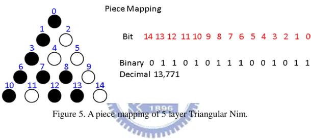
In order to identify the value of a given position in all the 2k(k+1)/2 bits, Hsu [33] simply used a k(k+1)/2-bit binary number as a position identifier. In the position identifier, each bit indicates whether a corresponding piece exists. The corresponding pieces to bits are designated by a piece mapping in advance. For example, in Figure 5, a piece mapping is shown, and a position of 5 layer Triangular Nim is identified as 011010111001011, equivalent to 13,771 in decimal, by a piece mapping. The initial position of 5 layer Triangular Nim is 111111111111111, all 1s. The initial positions for other layer Triangular Nim are all 1s, too.
Figure 5. A piece mapping of 5 layer Triangular Nim.
For a piece mapping, a legal move, removing some consecutive pieces, can also be represented by a k(k+1)/2-bit binary number corresponding to these removed pieces. For example, for the piece mapping in Figure 5, 000000000001011 is a legal move that removes the top three pieces at 0, 1 and 3. Since a legal move must remove consecutive pieces in a row or diagonal, the move at 1, 3 and 7 and the one at 1 and 8 are illegal. In [33], Hsu
derived that the total number of moves is k2(k+1)/2 in k layer Triangular Nim. Hence, the
number of legal moves is 75 for 5 layer Triangular Nim, while the number is 405 for 9 layer Triangular Nim. Thus, the time complexity for k layer Triangular Nim is roughly O(k32k(k+1)/2).
For a given position P, assume that a move M is legal in P. The bits with 1 in M must be 1 in P, too. We can use the following simple bit-wise operation to detect whether M is a legal move in P: The bit-wise AND operation on P and M is still M. In addition, we can also easily derive the position after the move M, by using bit-wise operations to remove all 1s of
M from P. Namely, the new position P' is P M, where is a bit-wise exclusive OR operation. For simplicity of discussion, P' is called a child of P, and P is the parent of P'.
For Triangular Nim, the backward induction approach is to derive V(P) from P = 0 to
2k(k+1)/2 – 1. V(P) denotes the value of a given position P. An important property is: The values V(P') for all children P' of P must have been evaluated, before the value V(P) is evaluated.
In [3][33] the researchers simply used a forward checking method to evaluate V(P). Initially, the position 0 is a P-position in the normal play, that is, V(0) = 0, while it is an N-position in the misère play, that is, V(0) = 1. When scanning to the position P, evaluate
V(P) from the values V(P') for all of its children P' by the two rules in Section 2.1.
2.2.2 Retrograde Method
The research in [47] used a more efficient method, a kind of retrograde method, which is also used in this thesis. Initially, the value V(0) is initialized as the forward checking method. In addition, all the other V(P) are initialized to 0. Then, the retrograde method also
follows the backward induction approach to visit position P from position 0 to 2k(k+1)/2 – 1
and perform the following update operation when visiting P.
By induction, we can show that the above operation satisfies the following property: When position P is visited, the value V(P) indicates the correct value. Assume that the properties are satisfied for all of its children. Then, if some child P' is a P-position, V(P) is set to 1 when visiting P' based on the above operation. This is correct since the position P is indeed an N-position based on the first rule in Section 2.1. If all children are N-positions,
V(P) remains 0. This is also correct since P is indeed a P-position based on the second rule.
Thus, it is concluded that the above property is satisfied.
The retrograde method is very efficient for the following reason. The above update operation is done only when the position P is a P-position (a loss to the next player to move). Most importantly, the loss rate, the number of P-positions to that of all positions, is normally low. The loss rate is only 6.0% for 8 layer Triangular Nim according to [47], while the loss rate is only 5.0% for 9 layer Triangular Nim according to the experiments in Section 2.4. That is, the computation times can be reduced by a factor of 20 or so.
2.3 Solving Approach
This section presents our approach to strongly solve 9 layer Triangular Nim. In our approach, we use the retrograde method and also propose some new methods for efficient data structures and removing redundancies, respectively described in Subsections 2.3.1 and 2.3.2.
2.3.1 Data Structures and Algorithms
Since 9 layer Triangular Nim requires a huge amount of memory (4 terabytes for the design described in Subsection 2.2.1), the memory space must be cut into disjoint blocks to make it feasible to process. To facilitate identifying the blocks, we let the most significant
bits of position identifiers be the block identifier. For simplicity of discussion, the block representation in 8 layer Triangular Nim is illustrated in the rest of this subsection.
(a) (b) (c)
(d) (e) (f)
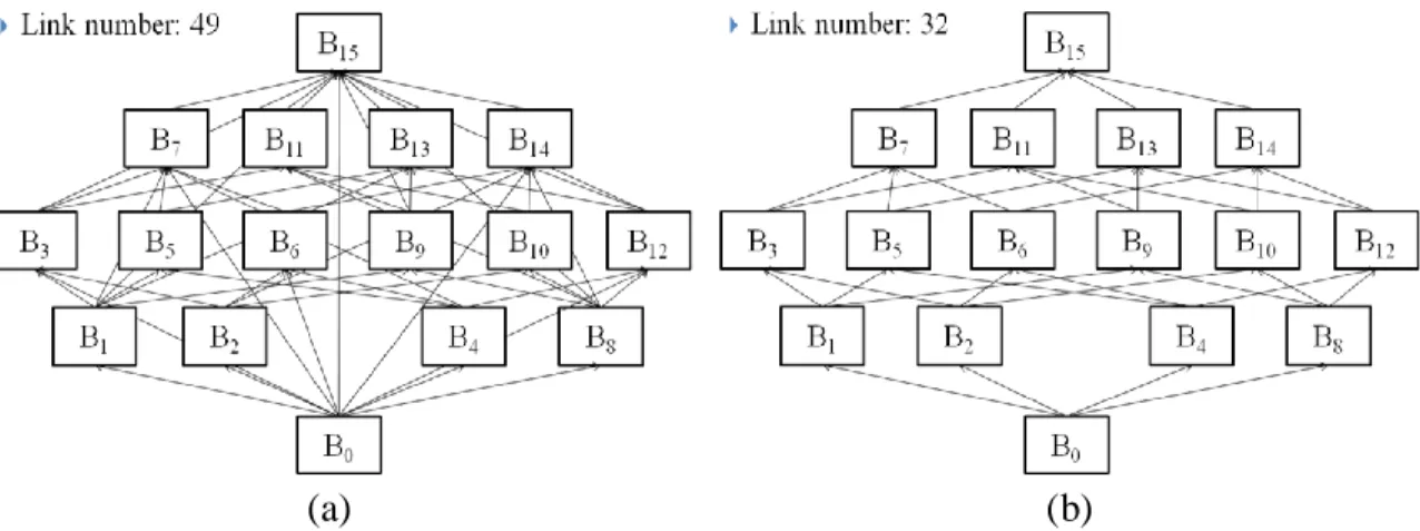
Figure 6. Six block representations for 8 layer Triangular Nim.
As described in Subsection 2.2.1, 8 layer Triangular Nim requires 236 bits, equivalent
to 233 bytes or 8 gigabytes. Assume to cut the memory space into 16 blocks, each with 512
megabytes. Then, the most four significant bits in the position identifier are used to indicate
the block identifier (Block ID or BID), 0 to 15. The 16 blocks are denoted by B0, ..., B15.
From the piece mapping described in Subsection 2.2.1, four pieces are designated as the bits of block identifier. The four pieces are called Block-ID pieces or BID pieces. For example, two such block representations using different BID pieces, marked with double cycles, are shown in Figure 6 (a) and (b). Other block representations using six BID pieces are shown in the rest of Figure 6.
Following the backward induction approach (in Subsection 2.2.1), we visit positions
from B0 to B15. Now, the next question is how to evaluate each block. Let us still follow the
approach as the retrograde method. We need to update the values in Bi+1, …, B15, when
visiting Bi. However, since the system memory (like RAM) may not be able to include all
blocks, we use the following operations when visiting the block Bi.
1. Load the block Bi (into the system memory).
2. Evaluate the values of Bi as follows.
a. Evaluate all positions P inside Bi by following the retrograde method.
Namely, for each P with V(P) = 0, set V(Ppar) = 1 for all of its parents Ppar
inside Bi.
b. Restore the block Bi into the peripheral memory like hard disks.
3. For all j > i, repeatedly perform the following.
a. Load the block Bj.
b. For each position P in Bi with V(P) = 0, set V(Ppar) = 1 for all of its parents
Ppar in Bj.
c. Restore the block Bj.
The above operations can be separated into different jobs. The operations 1 and 2
together, called intra-block update on Bi, is to update Bi itself. The operations 1 and 3
together for each j, called inter-block update from Bi to Bj, is to update Bj from Bi. For
inter-block updates from Bi to Bj, the block Bj is called a parent of Bi, or Bi is the child of Bj.
The above operations can be further improved by saving the restore operations in the inter-block updates (at Step 3.c), if we use a forward-checking method in the block level,
instead of a retrograde method in the block level. Namely, all inter-block updates from Bi to
Bj are done when visiting block Bj, not when visiting block Bi. The improved algorithm is
modified as follows.
1. Initialize the block Bj .
2. For all i = 0 to j–1, repeatedly perform the following inter-block updates.
a. Load the block Bi.
b. For each position P in Bi with V(P) = 0, set V(Ppar) = 1 for all of its parents
Ppar in Bj.
3. Process the intra-block update on Bj as follows.
a. Evaluate all positions P inside Bj by following the retrograde method.
Namely, for each P with V(P) = 0, set V(Ppar) = 1 for all of its parents Ppar
inside Bj.
b. Restore the block Bj into the peripheral memory like hard disks.
The above operation for 8 layer Triangular Nim requires 16 intra-block updates and 120 (=15×16/2) inter-block updates. In fact, the number of inter-block updates can be far below the above number. For example, for the block representation in Figure 6(a), no
operations are required for the inter-block update from B0 to B5, since it is impossible to
(a) (b)
Figure 7. Inter-block updates of the block representations in Figure 6 (a) and (b), respectively.
The number of required inter-block updates is usually small if the BID pieces are distributed sparsely, and large if the BID pieces are grouped. After our analysis, the number of required inter-block updates is 49 for the one in Figure 6(a), and 32 for the one in Figure 6(b). Figure 7 shows the inter-block updates for the two block representations, respectively. Usually, the smaller number of required inter-block updates is, the better performance is. This is also shown in our experiment in Section 2.4.
2.3.2 Removing Redundancy
Due to symmetry and rotation, we do not have to evaluate all the positions. However, it is hard to save space for all symmetric and rotated positions directly, since it is hard to
identify saved bits in our data structure shown in Subsection 2.3.1. Fortunately, it becomes
easier to save space on blocks.
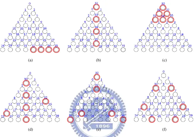
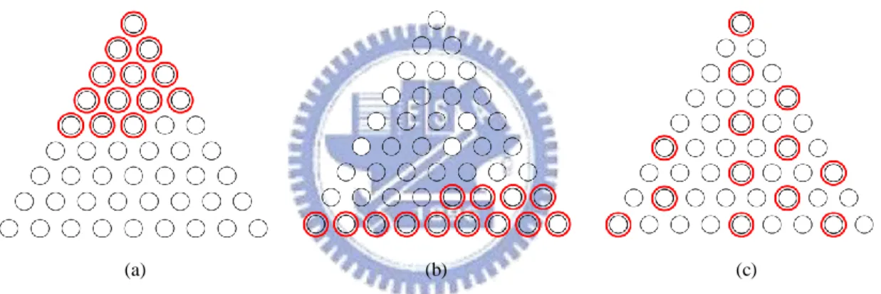
Let us illustrate the block representation with six BID pieces shown in Figure 6(f) and the blocks, B1, B2, B4, B8, B16 and B32, shown in Figure 8 (below). Due to symmetry and
B1, by finding the corresponding mirrored or rotated position values, and vice versa. Here,
B1 is said to be an isomorphic block of B2, and vice versa.
All of the six blocks shown in Figure 8 are actually isomorphic. Thus, it is sufficient to
evaluate the values of one block, say B1, only. And, we can get the values of other blocks
from the values of B1. These blocks form an isomorphic group of blocks.
In an isomorphic group of blocks, we can simply choose to evaluate the block with
smallest BID for simplicity. For example, in the group shown in Figure 8, we choose B1 to
evaluate. For the improved algorithm in the previous subsection, we add the following rules.
(a) (b) (c)
(d) (e) (f)
Figure 8. Six rotated and mirrored blocks.
1. When visiting Block Bi, skip it if there exists another isomorphic block with smaller
BID.
2. When making an inter-block update from Bi to Bj, access Bi' instead of Bi, if Bi' is the
In the second rule, when accessing block Bi, the block Bi' (with the smallest BID) must
be available, since we evaluate blocks from the lower BID to higher. In the rule, when
accessing positions in Bi, access the corresponding positions in Bi' according to the
directions of rotation and mirroring.
(a) (b) (c)
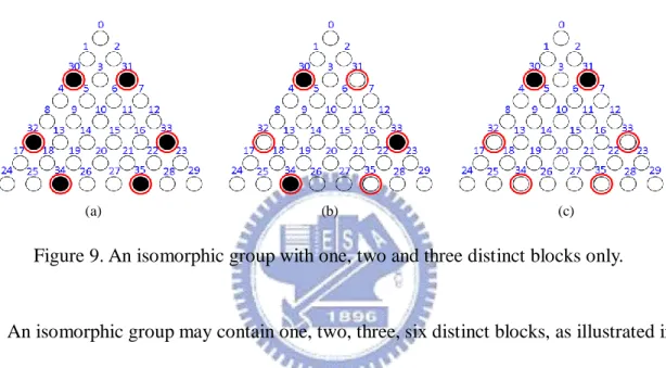
Figure 9. An isomorphic group with one, two and three distinct blocks only.
An isomorphic group may contain one, two, three, six distinct blocks, as illustrated in Figure 9(a), Figure 9(b), Figure 9(c), and Figure 8(a), respectively. Since an isomorphic group contains at most six distinct blocks, we can reduce the space by a factor of at most six. For the block representation (in both Figure 8 and Figure 9), the number of isomorphic groups with one distinct block is 2, that with two is 1, that with three is 6, and that with six is 7. Thus, for this block representation, we need to evaluate 16 blocks, among all the 64 blocks. Thus, we can save the space by a factor of four in this case.
The space saving rate grows higher and approximates to 6, if the block representation is well designed with large number of BID pieces. For example, for the block representation for 9 layer Triangular Nim shown in Figure 13(b), the number of isomorphic groups with one distinct block is 16, that with two is 8, that with three is 496, and that with six is 5,208.
Thus, for this block representation, we need to evaluate 5,728 blocks only, among all the 32,768 blocks. The space is reduced by a factor of 5.72, approximate to 6. More specifically, we can reduce the space from 4 terabytes to 716 gigabytes.
2.4 Experimental results
In this section, all experiments were done on a 4 cores personal computer equipped with Intel® Core™ 2 Quad CPU Q6600, 2.4GHz CPU, 8 gigabytes RAM and 6 terabytes hard disks with RAID, which had been used in the desk-top system [67]. We used a simple parallel method to exploiting the parallelism of the four cores as follows. Whenever a core
is idle, we choose a block Bi which has not been evaluated yet and whose children have
been evaluated. However, since parallelism is not the goal of our destination, we used the total times aggregated from the four cores.
Since it takes a huge amount of computation time for solving 9 layer Triangular Nim, we first investigate 8 layer Triangular Nim in Subsection 2.4.1. Then, based on the experiences for 8 layer Triangular Nim, we solve 9 layer Triangular Nim in Subsection 2.4.2.
2.4.1 Eight Layer Triangular Nim
This subsection investigates how to solve 8 layer misère Triangular Nim. We used the six block representations in Figure 6 as our testing cases. We used (a), (b), (c), (d), (e) and (f) to indicate the six representations respectively.
Table 1 shows the experimental results, using the method without removing redundancy as described in Subsection 2.3.1. Without removing redundancy, the total memory space requires 8 gigabytes for all cases. Table 1 clearly shows that the block
representations with the less numbers of inter-block updates are more efficient, since the overhead for inter-block updates becomes smaller. Due to the overhead for inter-block updates, the block representations with larger block sizes tend to run faster. On the other hand, the block size cannot exceed the physical or virtual memory size of the operating systems. Thus, this is a tradeoff for the block size.
Table 2 shows the experimental results with removing redundancy. This table does not include the cases (a), (b) and (d), since the results are the same as Table 1. Both cases (a) and (d) are not symmetric and rotatable. Although the case (b) is symmetric, all the isomorphic groups contain one block only, and therefore the results are the same as Table 1.
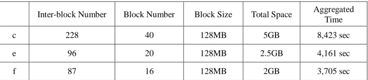
In Table 2, both cases (e) and (f) perform apparently more efficiently than the case (c), since the case (c) does not remove the redundancy caused by rotation. The case (f) performs more efficiently than the case (e), since both the number of blocks and the number of inter-block updates are smaller.
From the above experiments, we observe that the most important factor for high performance is to remove redundancy, and then to reduce the number of blocks or the number of inter-block updates. From the observation, we solve 9 layer Triangular Nim.
Inter-block Number Block Number Block Size Total Space Aggregated Time
a 49 16 512MB 8GB 8,992 sec b 32 16 512MB 8GB 8,472 sec c 360 64 128MB 8GB 13,453 sec d 208 64 128MB 8GB 11,042 sec e 288 64 128MB 8GB 12,339 sec f 336 64 128MB 8GB 13,128 sec
Table 1. Experimental results for the block representations without removing redundancy in Figure 6.
Inter-block Number Block Number Block Size Total Space Aggregated Time
c 228 40 128MB 5GB 8,423 sec
e 96 20 128MB 2.5GB 4,161 sec
f 87 16 128MB 2GB 3,705 sec
Table 2. Experimental results for three block representations with removing redundancy in Figure 6.
From the above experiments, we strongly solved all positions of 8 layer Triangular Nim with both normal and misère play. The results show that both initial positions for both normal and misère play are N-positions. The first player wins both by making the moves shown in Figure 10 for the normal play and those in Figure 11 for the misère play.
Figure 10. The moves to win in 8 layer normal Triangular Nim.
2.4.2 Nine Layer Triangular Nim
In this subsection, we first investigated the block representations with 13 BID pieces, three of them shown in Figure 12 (below). Although each block requires a large block size, 512 megabytes, these BID pieces cannot form symmetry or rotation so that we cannot remove redundant blocks as described in Subsection 2.3.2. Among the three in Figure 12, the one in Figure 12(c) has the least number of inter-block updates. Unfortunately, since it is still not symmetric and rotatable, it took 32.31 days on four cores (129.21 days on one core) to finish the whole computation in Table 3.
(a) (b) (c)
Figure 12. Three block representations with 13 BID pieces.
Inter-block Number
Blocks
Number Block Size Total Space
Parallel Computation Time Aggregated Time a 121,600 8,192 512MB 4TB N/A N/A b 107,024 8,192 512MB 4TB N/A N/A c 88,064 8,192 512MB 4TB 32.31 days 129.21 days
(a) (b) (c)
Figure 13. Three block representations with 15 BID pieces.
Inter-block Number
Blocks
Number Block Size Total Space
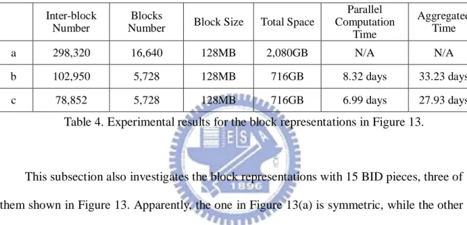
Parallel Computation Time Aggregated Time a 298,320 16,640 128MB 2,080GB N/A N/A b 102,950 5,728 128MB 716GB 8.32 days 33.23 days c 78,852 5,728 128MB 716GB 6.99 days 27.93 days
Table 4. Experimental results for the block representations in Figure 13.
This subsection also investigates the block representations with 15 BID pieces, three of them shown in Figure 13. Apparently, the one in Figure 13(a) is symmetric, while the other two are symmetric and rotatable. Due to symmetry and rotation, the number of blocks can be reduced by a factor of near 2 for the first and near 6 for the other two. The results showed that the computation times for the second and third are reduced to 8.32 days and 6.99 days as shown in Table 4, respectively. The third is slightly better than the second, since the number of inter-block updates is smaller as shown in Table 4. In brief, from the one in Figure 12(c) to that in Figure 13(c), we reduce the memory by a factor of 5.72 and the computation time by a factor of 4.62.
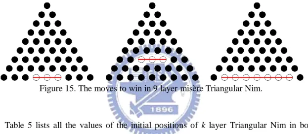
From the above experiments, we strongly solved all positions of 9 layer Triangular Nim in both normal and misère play. The results also show that both initial positions in both normal and misère play are N-positions. The first player wins both by making the moves
shown in Figure 14 for the normal play and those in Figure 15 for the misère play.
Figure 14. The moves to win in 9 layer normal Triangular Nim.
Figure 15. The moves to win in 9 layer misère Triangular Nim.
Table 5 lists all the values of the initial positions of k layer Triangular Nim in both normal and misère, where k is 1 to 9. This table shows that the first player tends to win or that the initial positions tend to be N-positions. This is because the ratio of the number of P-positions to that of N-positions tends to be low, that is, most positions are N-positions.
We also analyzed the ratio in both normal and misère in Figure 16 for all k layer Triangular Nim, where k is 1 to 9. From the Figure 16, the ratios get smaller for large k. For 9 layer Triangular Nim, the ratio is 5.0% only. This explains why most of initial positions are N-positions. In addition, since most positions are N-positions, this shows that the retrograde method is clearly superior.
k k Layer Normal Triangular Nim k Layer Misère Triangular Nim 1 Win Loss 2 Loss Win 3 Win Loss 4 Win Win 5 Win Loss 6 Win Win 7 Win Win 8 Win Win 9 Win Win
Table 5. The result of k layer Triangular Nim.
Figure 16. The ratio of the number of P-positions to that of N-positions.
2.5 Conclusion
We summary our contributions in this chapter as following lists.
This thesis also proposes some methods to improve the performance, such as designing data structures in blocks, using the retrograde method, removing redundancy and selecting the block representation with the less number of inter-block updates. Especially, by removing redundancy, we reduce the memory by a factor of 5.72 and the computation time by a factor of 4.62 using personal computer equipped with Intel® Core™ 2 Quad CPU Q6600, 2.4GHz CPU, 8 gigabytes RAM.
Our experiment result also shows that the ratio of the number of P-positions to that of N-positions is low, 5.0% for 9 layer Triangular Nim. Due to the low ratio, the retrograde method does perform well when compared with the traditional forward checking.
We also got all game values of 6 layer Triangular Nim positions in normal play. During the game play, if the board is divided to several subgames which are all under 6 layer Triangular Nim positions, we can calculate the sum of game values of subgames to quickly judge who to win by Sprague–Grundy Theorem.
Chapter 3 XT Domineering: A New Combinatorial
Game
This chapter introduces a new combinatorial game of XT Domineering. We use combinatorial game theory (CGT) to calculate the game values of all sub-graphs of 3×3 squares and show that each sub-graph of 3×3 squares is a linear combination of 8 elementary infinitesimals.
3.1 Introduction
Domineering, designed by Göran Andersson [27], is one of combinatorial games that were based on the model. In an m×n Domineering, two players alternatively place 1×2 and 2×1 domino at a position, if there exists such a vacancy in a board with m×n squares. One player is allowed to place 1×2 domino only, while the other is 2×1 domino only. The one who cannot place domino loses.
In the past, many Domineering problems were solved. The general Domineering problem of 2×n board for all odd n was solved by Berlekamp [5]. The researchers in [9] used the technique of transposition tables to solve the 8×8 board. Subsequently, the researchers in [44] found out the results for boards of width 2, 3, 5, and 7 and some specific cases. Recently, Bullock solved the 10×10 board Domineering [12]. Furthermore, Cincotti developed three players Domineering on a three dimensional board [16][17].
This chapter introduces a new game named XT Domineering (named from eXTended
Domineering). XT Domineering, modified from the Domineering game, allows players to
place a 1×1 domino on an empty square s while unable to place a 1×2 or 2×1 domino in the connected group of empty squares that includes s. A connected group of empty squares is called an active group. After modifying the rule, players are allowed to place 1×1 domino on any square of an active group on which players are not allowed to place any dominos in the original Domineering game. For example, in XT Domineering, all 1×1 isolated vacancies in the board are allowed to be placed by more dominos. Thus, the move lengths in the new game are normally longer than those in Domineering. Thus, the game has higher game-tree complexity, based on the definition in [35].
This chapter also introduces the mathematical analysis of XT Domineering. In XT Domineering, each game position is actually an infinitesimal (as described in Section 3.4). In this chapter, we study several interesting infinitesimals in XT Domineering. This chapter calculates the game values of all sub-graphs of 3×3 squares and presents a rule to determine the outcome of any sum of these positions.
Section 3.2 reviews the combinational games including three subgroups of games. Section 3.3 reviews the game Domineering and introduces the new game, XT Domineering. Section 3.4 derives the game values of 3×3 XT Domineering, while Section 3.5 derives the outcomes of sums of 3×3 XT Domineering. Section 3.6 concludes this chapter.
3.2 Combinatorial Games
CGT [7] starts from a simple definition of game: A game is an ordered pair of sets of games. Since we are dealing with equivalence classes, for simplicity, we shall use the
There are several subgroups of combinatorial games whose addition and outcome properties are well-studied. Some of them are reviewed in the following subsections.
3.2.1 Numbers
A game G is called a number [7][20] if all the elements in GL and GR are numbers and
there is no element in GL greater than or equal to any element in GR. Some numbers are
illustrated as follows:
1 = {0 | }, …
n = {n – 1 | },… (13)
1/2 = {0 | 1}, …
m/2k = { (m – 1)/2k | (m + 1)/2k }. (14)
These numbers (integers and rationals) can be added as the usual ways. Numbers are well ordered, and their relations with 0 are clear. Hence, one can easily determine the outcome for any sum of numbers.
3.2.2 Nimbers
A game G is a nimber [8][31] if all the elements in GL and GR are nimbers and GL = GR.
Nimbers are defined as: *1 = { 0 | 0}, *2 = {0, *1 | 0, *1}, …
*n = {0, *1, *2, …, *(n – 1) | 0, *1, *2, …, *(n – 1)}. (15)
For simplicity, *1 is also denoted as * and named star. The special nimber with infinite options:
☆ = {0, *1, *2, … | 0, *1, *2, …}. (16)
is named remote star.
For each non-zero nimber, the first player can win a game. That is, each non-zero nimber is confused with 0. Hence one can easily determine the outcome of any sum of numbers [31][60]. From this, two well-known properties are (1) *n + *n = 0, and (2) {*n | *n} = 0.
3.2.3 Sumbers
For each number d, there is a corresponding up defined as [7][20][36].
↑(d) = {↑(dL) , * | ↑(dR
) ,*}. (17)
The negation of up is called down.
↓(d) = ↑(d). (18)
A property between all ups and stars [7][20] is: for all numbers d > 0 and n > 1, we have
↑(d)n and↑(d)☆ (19)
↑(d)*(or ↑(d)*) (20) We use the notation m.↑(d) to denote the sum of m copies of ↑(d). A sumber S (cf. [39]) is a sum of ups, downs and stars(*).
S = ∑k=1,n ak↑(dk) + a0*. (21)
where ak are integers and dk are numbers, 0 < k n. Without loss of generality, in (21),
we assume 0 < d1 < d2 < …< dn and a0=0 or 1.Clearly, sumbers are closed under addition.
We use the notation G << H to denote that the sum of any number of copies of G is less than H. The sumbers have the following properties:
0 < ↑(d1) < ↑(d2), (22)
0 << ↑(dn+1) – ↑(dn) << ↑(dn) – ↑(dn-1), (23)
↑(dn+1) + ↑(dn+1) – ↑(dn) > *, (24)
where 0 < d1 < d2 < …< dn < dn+1 < …. These properties are sufficient to determine the
outcome of any sum of sumbers. The research in [39] provides a simple rule to determine the outcome of (21):
S > 0 if and only if ∑k=1,n ak > a0 or (∑k=1,n ak = a0, and a1 < 0),
where a0 is either 1 or 0. Note that the net number of ups is greater than the net number
of *, or the net number of ups equals the net number of * and the smallest up has a negative coefficient.
For example, consider SA = –↑(3) + 3.↑(1) + *. In SA, the net number of ups (=2) is
greater than the net number of * (=1), thus SA >0. Consider SB = –↑(3) + 3.↑(2) – ↑(1) + *. In
has a negative coefficient (= –1), thus SB >0. Consider SC = ↑(3) – 2.↑(2) + 2.↑(1) + *. In SC,
the net number of ups (=1) equals the net number of * (=1), but the smallest up (=↑(1)) has
a positive coefficient (=2), thus SC ≯ 0. Let “≯” denote “not greater than”.
3.2.4 Infinitesimal and Atomic Weight
A game G is called an infinitesimal if and only if G is less than any positive numbers and greater than any negative numbers. Nimbers and sumbers are all infinitesimals.
Researchers in [7][20] introduced the definition of atomic weight. If G = {Ga, Gb, Gc, …| Gd,
Ge, Gf,…} where Ga, Gb, Gc, Gd, Ge, Gf, … have atomic weight a, b, c, d, e, f, …, then the
atomic weight of G is
G0 = {a – 2, b – 2, c – 2,… | d + 2, e + 2, f + 2,…}
unless G0 is an integer and either G > ☆ or G < ☆. In these exceptional cases, if G >
☆ then the atomic weight of G is the largest integer <| d + 2, e + 2, f + 2, …, and if G < ☆ then the atomic weight of G is the least integer |> a – 2, b – 2, c – 2, ….
According to the above definition, each nimber has atomic weight 0; each up has atomic weight 1.
Two important properties [7][20] about atomic weights are described as follows.
1. The atomic weight of a sum of games equals to the sum of the atomic weights of the
games.
2. If the atomic weight of a game is greater than or equals to 2, then Left wins the game.
On the other hand, if it is less than or equals to –2, then Right wins the game. However, there are no general rules when the atomic weight is between –2 and 2.
For example, ↑ + ↑(2) has atomic weight 2, hence Left can win the game; ↓ + ↑(2) + ↓(3) + ↓(4) – ☆ + * – *(3) has atomic weight –2, hence Right can win the game. Thus, for some games, we can determine the winners by computing the atomic weight of sub-games, instead of searching complex trees.
3.3 Domineering and XT Domineering
Domineering (also called Stop-Gate or Crosscram) [27] is a mathematical game played on a board with n×n squares. Two players have a collection of 1×2 and 2×1 dominos which they place on the grid in turn, covering up squares. One player, Left, plays first and places domino vertically (1×2), while the other, Right, places horizontally (2×1). The first player who cannot place a domino loses the game.
Figure 17. Middle game of 6×6 Domineering.
As the game progresses, the original n×n squares may be partitioned into a set of disjoint sub-positions. Figure 17 shows a graph in the middle of a 6×6 Domineering. It contains 5 disjoint sub-positions shown in Figure 18.
.
Figure 18. Sub-positions of the graph in Figure 17
In terms of CGT, the game G in Figure 17 is a sum of sub-positions A, B, C, D, and E, i.e., G = A + B + C + D + E. Note that by rotating position D 90° counter clockwise, one can get position E. In general, rotating a Domineering position 90° (either clockwise or counter clockwise) will result a negation of the original position, and reflecting a Domineering position with respect to a vertical axis or horizontal axis will not change the game value of the position. Hence, E = -D, and G = A + B + C.
Domineering attracted many combinatorial game researchers because the game contains many numbers, switches of numbers, and complicated hot positions.
Figure 19 (below) shows the game values of the positions in Figure 18. Note that the derivations are based on [5] and the details of derivations are therefore omitted in this thesis. By summing up the values, we have G = 3/4 + { 1 | -1}-1 =-1/4 + { 1 | -1} = {3/4 | -5/4}, thus the first player can win the game. This illustrates the power of using combinatorial theory, since we can derive the result without tree search as many board games do. A simpler example is illustrated in Appendix A.
Figure 19. Some game values in Domineering.
A
B
C
D
E
XT Domineering is modified from the Domineering game by changing the rule to allow a player placing a small (1×1) domino on a sub-position while unable to place his big domino (1×2 or 2×1) in the sub-position in the original Domineering game. For example, consider sub-position C in Figure 18. In Domineering, Left cannot place a domino vertically (1×2) at sub-position C, while in XT Domineering, Left is allowed to place a 1×1 domino at
sub-position C. More specifically, sub-position C has the value { | 0} = - 1 in
Domineering, and {{0 | 0} || 0} = {* | 0} = ↓ in XT Domineering. Note that Left is not allowed to place a 1×1 domino at a position while he is able to place a 1×2 domino at that position and Right is not allowed to place a 1×1 domino at a position while he is able to place a 2×1 domino at that position. For example, both players are not allowed to place 1×1 domino at positions A, B, D and E in Figure 18.
Since XT Domineering has at least the same number of options as Domineering and allows more moves (e.g., on 1×1 vacancies), XT Domineering has higher game-tree complexity [35].
Note that each player has at least one option at any non-empty position in XT Domineering. This nature prevents the occurrence of non-zero numbers and ensures that each position in XT Domineering is an infinitesimal. One of the major motivations of this thesis is to see what kind of infinitesimals may be shown up in this game.
3.4 Game Values of 3×3 XT Domineering
For XT Domineering with 1×n squares, the games have periodic values with period length 8, {0, *, ↓, ↑, *, 0, ↑*, ↓*} [38]. This is in fact a partisan octal game [51]. In this
After excluding non-connected sub-graphs, rotated negation sub-graphs, or reflected equivalence sub-graphs, there are 34 distinct positions. The game values of these distinct positions are derived based on the above inequalities (6) to (24), and shown in Table 6. Each position in Table 6 is a linear combination of the following 8 elementary games:
↑ = {0 | *}, ↑+ = {↑ | *}, ↑/2 = {↑↑* | ↓* ★ = {0, ↑* | ↓*, 0} */2 = {↑↑ | ↓↓*}, (*/2) + = {↑↑, ↑↑* | ↓↓*} ◇ = {↑↑↑* | ↓↓↓* }
For simplicity, let ↑↑ indicate ↑ + ↑, and similarly for ↑↑*, ↑↑↑*, etc.
The games *, ↑ and ↑+ (=↑(2)) have been introduced in Section 3.3. * has atomic
weight 0 (as described in Subsection 3.2.4), while ↑ and ↑+ have atomic weight 1 each. We
use the symbol ↑2 to denote ↑+ - ↑.
↑2 = ↑ -↑ .
From inequality (23), we have ↑ >> ↑2
> 0.
The game ↑/2 (half up), as the name suggested, has atomic weight 1/2 and the following properties:
↑/2 + ↑/2 = ↑. ↑/2 > ↑2
.
The game ★ (black star) has atomic weight 0 and with property similar to nimbers:
★ + ★ = 0,
★ || *(n), for integer n > 0
The game */2 (half star), as the name suggested, has the following property:
*/2 + */2 = *.
The game */2 has atomic weight {0 | 0} = *, since the atomic weight of ↑↑ is + 2 and that of ↓↓* is –2.
The game (*/2)+ (half star plus), as the name suggested, is just slightly greater than */2
and has atomic weight {0, 0 | 0} = *. The difference between (*/2)+ and */2 is named △*:
△* = (*/2)+ - */2 > 0.
Since the atomic weight of both (*/2)+ and */2 are *, the atomic weight of △*
equals * – * = 0.
The game ◇ (diamond) has atomic weight {1 | –1}. Since the incentive of ◇ (diamond) is greater than the ones of all the other 7 elementary games, ◇ should always be played first among the 8 elementary games. Diamond also has the property below:
No. Position Value No. Position Value P1-1 * P6-1 */2 P2-1 ↑ P6-2 */2 P3-1 0 P6-3 ↑↑* P3-2 ↓ P6-4 ↑+ P4-1 * P6-5 ↑/2 P4-2 * P6-6 ★ + * P4-3 ↑↑* P6-7 0 P4-4 * P6-8 0 P5-1 ★ P7-1 * P5-2 * P7-2 ↑* P5-3 ↑↑ P7-3 ↑ P5-4 ★ P7-4 ↑* P5-5 ↑↑ P7-5 * P5-6 ↑ P7-6 0 P5-7 0 P7-7 * + (*/2)+ P8-1 * P8-3 0 P8-2 ◇ P9-1 0