用於擺置繞線流程的可繞度和效能最佳化技術

國立交通大學資訊學院資訊科學與工程研究所

博士論文

Graduate Institute of Computer Science and Engineering

College of Computer Science

National Chiao Tung University

Doctoral Dissertation

用於擺置繞線流程的可繞度和效能最佳化技術

Optimizing Routability and Performance of Placement and

Routing Flow for Nanometer Designs

劉文皓

Wen-Hao Liu

指導教授:李毅郎 博士

Advisor: Yih-Lang Li, Ph.D.

中華民國一百零二年一月

January, 2013

i

摘要

近年來，隨著奈米技術的進步，晶片中的元件越來越多，同時繞線的

難度也越來越高。晶片的可繞性(Routability)成為眾人所觀注的議題。在

該議題上，全域繞線(Global Routing)扮演著重要的角色。在電路實體設

計(Physical Design)的流程中，全域繞線上承元件擺放(Placement)，下

啟細部繞線(Detailed Routing)。一個快速的全域繞線器能提供擁擠度

(Congestion)的資訊給擺放器，讓擺放器擺出較容易繞線的布局。此外，

若全域繞線器能有效的解決繞線擁擠度的問題，細部繞線的負擔和所需

時間可以大幅降低。當全域繞線器和擺放器合作時，全域繞線器如何快

速且準確的回報擁擠度資訊給擺放器是一個重要的議題。另一方面，當

全域繞線器扮演細部繞線器的指導者角色時，全域繞線結果的品質就顯

的格外重要。若細部繞線器能根據一個高品質的全域繞線結果進行細部

繞線，將會提升細部繞線結果的品質，並大縮短細部繞線的時間。這篇

論文提出了兩個全域繞線器: Grace是個快速的全域繞線器，適合擔任擁

擠度預估器; NCTU-GR 2.0能產生高品質的繞線結果來指導細部繞線，

其繞線結果較不擁擠且有較短的線長。此外，為了將Grace應用於業界，

我們增加了許多功能於Grace中來滿足業界的需求。在擺放和繞線的中間

階段，我們結合了擺放器和全域繞線器，提出了一個可繞性優化器

(Routability Optimizer)。若給予一個布局結果，該優化器可以重新擺放

其中的元件，讓該布局更容易被繞線，進而得到更好的繞線結果。最終，

在進行細部繞線前，我們還提出了一個三維繞線改善器，將全域繞線的

結果在做進一步的改善，此舉可以更進一步的降低細部繞線器的時間和

負擔。

ii

Abstract

Routability has become one of most critical issues to successfully achieve design closure.

To address this issue, global routing plays an important role in the placement and routing

flow. During the placement stage, a fast global router can serve as a routing congestion

estimator to guide that placers improve the routability of placement solutions; however,

traditional global routers are too slow to offer quick but accurate congestion estimation. In

the routing stage, the duty of a global router is to identify a global routing result to guide

downstream detailed routers. The runtime of the detailed router can significantly reduce if

the global routing result has well optimized congestion and wirelength.

In this dissertation, two global routing engines are proposed, Grace and NCTU-GR 2.0.

Grace is a fast global router to serve as a fast routing congestion estimator, adopts the

proposed unilateral monotonic routing and hybrid unilateral monotonic routing to replace

time-consuming maze routing in its routing flow, and invokes a congestion-aware bounding

box expansion scheme to avoid over-expanding the searching regions to achieve high

speedup. Moreover, in order to use Grace in the industrial flow, Grace have been enhanced

to tackle the layer directive and scenic constraints for considering the timing issue.

Another proposed global router NCTU-GR 2.0 can generate high-quality global routing

results to guide the downstream detailed router. The proposed bounded-length maze

routing avoids producing redundant detours to save routing resource; rectilinear Steiner

minimum tree aware routing scheme can guide NCTU-GR 2.0 to build a routing tree for

each multi-pin net with shorter wirelength; a dynamically adjusted history cost function

highlights for NCTU-GR 2.0 which grid edges are critical routing resource that can be more

carefully allocated to the nets that really desire. Based on the proposed innovations to

carefully utilize routing resource, NCTU-GR 2.0 obtains shorter total wirelength and lower

iii

In addition, between the placement and routing stages, this dissertation presents an

incremental place-and-route tool called Ropt to optimize the routability of a given

placement solution. Rather than minimizing HPWL, Ropt directly improves routability by

minimizing the routing cost of nets, as the routing cost is defined in terms of global

congestion, local congestion and wirelength. In addition to using NCTU-GR 2.0 to evaluate

the routability of the placement solutions, this work also uses Wroute to obtain detailed

routing results of the optimized placement solutions for the evaluation of real routability.

Finally, the proposed post-3D-global-router called Post3DGR further refines the

wirelength, congestion, and via count of a given 3D global routing result. Post3DGR consists

of the 3D post routing stage and negotiation-based layer assignment stage. The 3D post

routing stage adopts an inherited history cost function to guide the routing, which can

greedily reduce total wirelength and vias. The negotiation-based layer assignment stage

re-assigns the routing layer for each wire to reduce via count. The negotiation-based layer

assignment can be extended to consider via overflow and antenna effect. Considering these

issues before detailed routing can ease the effort and runtime of subsequent detailed

iv

誌謝

能順利的完成這份論文，我最先要感謝的是我的父母-劉修添先生和

蘇素華女士。謝謝你們的支持，讓我能無後顧之憂的做自己喜歡的研究。

你們的身教和言教，是我能順利完成博士學位的最大原因。謝謝你們。

我希望將這份論文獻給我最親愛的父親和母親。

在我博士生涯中，謝謝李毅郎老師的細心且耐心的指導。我何等幸

運，因為經師多有，人師難得。謝謝你教導我做研究的方法和待人處事

的道理。這四年在你的教導下，我覺得我在很多方面都有大幅的進步，

特別是論文撰寫方面。四年前，我連一句文法正確的英文句子都寫不出

現。往往整篇論文都要經過你的大幅翻修，才能讓人讀懂。謝謝你花許

多精力批改我的論文和教導我如何寫論文。因為你的教導，這篇博士論

文才能順利完成。

謝謝Cheng-Kok Koh教授給我到普渡大學進行千里馬的機會。我在普

渡大學的這段時間，謝謝你關心我的生活，並跟我分享你的人生經驗。

在我們討論研究進度時，謝謝你能忍受我的破爛英文，並且不時的幫我

正音。我從你身上學到了有別以往的研究方法，並且更開擴了我的國際

觀。我相當感激並且慶幸能受到你的指導。當我在美國的期間，謝謝Cliff

Sze博士給我到IBM Austin Lab進行短期研究的機會。IBM Austin Lab一

直是我心中所響往的一流研究機構，在這裡，我很慶幸能和許多知名的

研究者共事。我在IBM的期間，學到了業界解決問題的方法，並且讓我

的英文的溝通能力大有進步。

一路走來，我要感謝的人實在是太多了。謝謝國小時的林蘭春老師，

國中時的張澄仁老師，高中時的徐英珠老師和黃玉慧老師。你們總是在

v

我做錯事時包容我、糾正我;在我意志消沉時鼓勵我、鞭策我。沒有你們

的教誨，就沒有今日的我。在我就讀博士期間，謝謝王廷基教授和張耀

文教授對我的照顧和經驗分享。我要特別感謝王廷基教授，我在研究上

遇到困難時，王廷基教授經常對我伸出援手。我還要感謝我的姑姑-劉虹

君女士，謝謝妳對我的照顧和愛護，妳在我的成長過程中扮演著十分重

要的角色。最後我要感謝我的女朋友-林珈竹，謝謝妳陪伴我走過研究所

的求學生涯，謝謝妳在我研究受挫時鼓勵我、聽我訴苦。有妳相伴的時

光，讓我的生活不再只是程式碼和論文，妳讓我的研究所生涯多了許多

美好的回憶。謝謝妳，我愛妳。

vi

Table of Contents

Chapter 1

Introduction...1

1.1 Overveiw of this Dissertation ...1

1.2 Background...4

1.2.1 Building Grid Graph and the Objectives of Global Routing...5

1.2.2 Net Decomposition ...6

1.2.3 Pattern Routing and Monotonic Routing ...7

1.2.4 Negotiation-based Rip-up and Rerouting (NRR)...7

1.2.5 Layer Assignment...8

1.2.6 Comparison of Recent Global Routers ...9

Chapter 2

Grace: A Fast Global-routng-based Routing Congestion Estimator ...10

2.1 Introduction...10

2.2 Problem Description ...11

2.3 The Proposed Algorithms for Accelerating Routing...12

2.3.1 Unilateral Monotonic Routing ...13

2.3.2 Hybrid Unilateral Monotonic Routing...17

2.3.3 Congestion-aware Bounding Box Expansion ...20

2.4 Design Flow of Grace...22

2.5 Experimental Results...23

2.5.1 Comparison between NCTU-GR 2.0 and Grace...24

2.5.2 Effectiveness of the Proposed Algorithms ...27

2.6 Summary ...28

Chapter 3

E-Grace: Enhancing Grace for Practically Industrial Designs ...29

3.1 Introduction...29

3.2 Preliminaries ...32

3.2.1 Problem Description ...32

3.2.2 Congestion Evaluation Metrics ...33

3.2.3 Previous Works ...33

3.3 Design Flow of E-Grace...34

3.3.1 Relaxation-Legalization Scenic Controlling Method ...36

3.3.2 TCR-driven R&R Scheme ...40

3.3.3 Throughput Controlling...42

3.4 Experimental Results...43

3.4.1 Compare E-Grace with other industrial RCE tools...43

3.4.2 Effectiveness of each Innovation in E-Grace ...45

vii

Chapter 4

Ropt: Optimization of Placement Solutions for Routability ...51

4.1 Introduction...51

4.2 Problem Description ...53

4.3 Case Study for Placement Solutions in DAC Contest ...54

4.3.1 Framework for Performing Detailed Routing ...55

4.3.2 Mismatch between Global and Detailed Routability...56

4.3.3 What Causes Routing Violations ...58

4.4 Proposed Routability Optmizer ...60

4.4.1 Local-Routability-Aware Global Routing Model ...60

4.4.2 Routing-cost-driven Global Re-Placement ...63

4.4.3 Legalization with Global Routing Preserved...66

4.4.4 Local Detailed Placement...67

4.5 Experimental Results...68

4.5.1 Global Routability: Evaluation by NCTU-GR 2.0 ...69

4.5.2 Effective Routability: Evaluation by Wroute...71

4.5.3 Comparison between Abacus and Our Legalizer...75

4.6 Summary ...76

Chapter 5

NCTU-GR 2.0: Global Routing with Bounded-Length Maze Routing ....78

5.1 Introduction...78

5.2 Problem Description ...80

5.3 Proposed Approaches to Improve Routing Quality ...81

5.3.1 BLMR ...81

5.3.2 RSMT-Aware Routing Scheme ...88

5.3.3 Dynamically Adjusted History Cost Function ...90

5.4 Design Flow of NCTU-GR 2.0 ...91

5.5 Experimental Results...94

5.5.1 Comparing Traditional Maze Routings with BLMR ...94

5.5.2 The Effectiveness of RSMT-aware Routing ...96

5.5.3 Comparison of Optimal-BLMR and Heuristic-BLMR ...96

5.5.4 Routing Result Comparison of Sequential Routers...97

5.6 Summary ...100

Chapter 6

Post3DGR: Post Optimization of 3D Global Routing Results ...101

6.1 Introduction...101

6.2 Problem Description ...104

6.3 Design Flow of Post3DGR ...104

6.4 Negotiation-based Layer Assignment (NLA)...107

viii

6.4.2 MCSNLA: Minimum-cost Single Net Layer Assignment...109

6.4.3 Congestion Cost Formulations...115

6.5 Experimental Results...117

6.5.1 Effectiveness of NLA...118

6.5.2 Effctiveness of Post3DGR ...119

6.5.3 Consideration of Antenna Effect...121

6.6 Summary ...122

Chapter 7

Conclusions and Future Works ...123

7.1 Conclusions...123

7.2 Future Works ...124

ix

List of Figures

Fig. 1.1 (a) A placement solution; (b) a global routing result; (c) a detailed routing result of

a design. ... 1

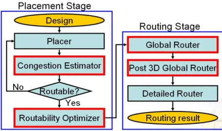
Fig. 1.2 Routability-driven placement and routing (P&R) flow... 2

Fig. 1.3 (a) partition a placement into a 3D array of G-cells; (b) model the 3D array of G-cells into a grid graph; (c) typical global routing flow... 5

Fig. 1.4. modern 3D global routing flow... 6

Fig. 1.5. Four-pin net decomposition ... 7

Fig. 2.1. (a) Vertically monotonic routing path; (b) horizontally monotonic routing path; (c) routing path combining vertically and horizontally monotonic routing. ... 12

Fig. 2.2. Example of VM routing... 14

Fig. 2.3. The proposed vertically monotonic routing algorithm... 15

Fig. 2.4. The pseudo code of hybrid unilateral monotonic routing algorithm ... 17

Fig. 2.5. Four path types in B with congested regions ... 18

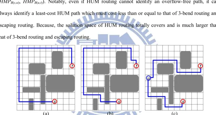
Fig. 2.6. (a) Routing result of 3-bend routing with two overflows; (b) routing result of escaping routing with an overflow; (c) routing result of the proposed HUM routing without overflows. ... 19

Fig. 2.7. Example of congestion-aware bounding box expansion... 20

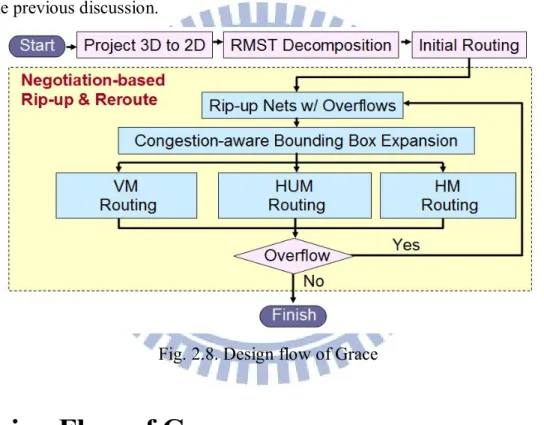
Fig. 2.8. Design flow of Grace ... 22

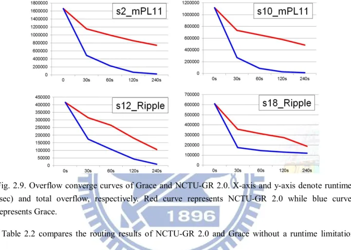
Fig. 2.9. Overflow converge curves of Grace and NCTU-GR 2.0 ... 25

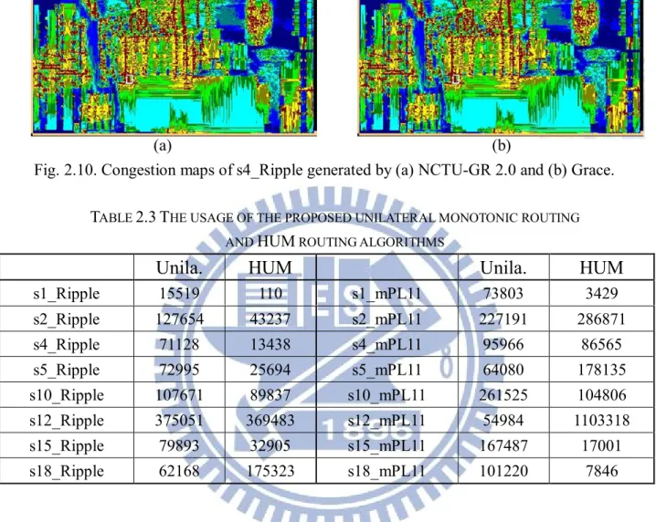
Fig. 2.10. Congestion maps of s4_Ripple generated by (a) NCTU-GR 2.0 and (b) Grace ... 27

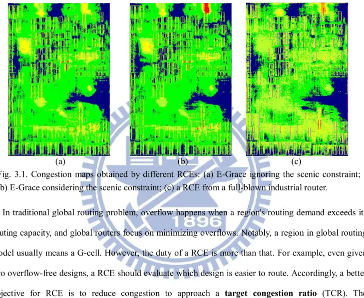
Fig. 3.1. Congestion maps obtained by different RCEs... 30

Fig. 3.2. Design flow of E-Grace... 34

Fig. 3.3. (a) the initial routing result of a net; (b) a segment exhausts all detour quotas, resulting another segment has no detour quotas to bypass congestion regions; (c) the routing result of the proposed R&R stage; (d) the routing result after the scenic legalization stage ... 36

Fig. 3.4. The routing result obtained by (a) the R&R stage; (b) the first iteration of the soft legalization phase; (c) the second iteration of the soft legalization phase ... 39

Fig. 3.5. Curve of cc(e) in Eq. (3.5) ... 41

Fig. 3.6. Congestions maps of Ind4 obtained by (a) CAind, (b) EGall, (c) GRind... 45

Fig. 3.7. Routing results of Ind11. (a) Minimizing overflows; (b) minimizing congestion ratio to approach 80%; (c) color scheme... 48

x

Fig. 3.8. Routing results of Ind11 (a) without extra blockages; (b) with 2% extra blockages;

(c) with 5% extra blockages ... 50

Fig. 4.1. Placement solutions of s19 obtained by (a) Ripple; (b) mPL; (c) SimPLR; (d) NTUplace... 58

Fig. 4.2. The local views of the most congested region in the placement solution of (a) mPL; (b) Ripple; (c) NTUplace ... 59

Fig. 4.3. Design flow of the proposed routability optimizer Ropt... 60

Fig. 4.4. Pseudo code of the algorithm for FOPG problem ... 64

Fig. 4.5. An example of the proposed heuristic algorithm for FOPG problem... 65

Fig. 4.6. Pseudo code of local detailed placement... 67

Fig. 5.1. (a) Maze routing within a bounding box; (b) maze routing without bounding box. ... 80

Fig. 5.2. (a) The search region of the net while L is set to 9; (b) two path candidates P1 and P2 from s to v; (c) ewk(v, t) denotes estimating wirelength from v to t in iteration k ... 83

Fig. 5.3. Relationship between the routing iteration number and the scaling factor ... 87

Fig. 5.4. Example of RSMT-aware routing scheme... 89

Fig. 5.5. Design flow of NCTU-GR 2.0... 92

Fig. 6.1. Gap of the recognition of good results between 2D routing with layer assignment and 3D routing ... 102

Fig. 6.2. MGR flow... 103

Fig. 6.3. (a) Design flow of Post3DGR. (b) Design flow of NLA ... 104

Fig. 6.4. Example of the quality improvement in Post3DGR ... 105

Fig. 6.5. The comparison between existing layer assignments and NLA ... 107

Fig. 6.6. An example of single net layer assignment ... 109

Fig. 6.7. The pseudo code of MCSNLA ... 111

Fig. 6.8. Procedure InitSol of MCSNLA ... 112

Fig. 6.9. Procedure EnumSol of MCSNLA... 112

Fig. 6.10. An example for constructing a 3D tree ti,3... 113

Fig. 6.11. An example of EnumSol ... 113

Fig. 6.12 The overflow reduction stage of NLA resolves overflow (OF) of adaptec2 at the cost of increasing vias ... 116

xi

List of Tables

Table 1.1 Recent global routing researches ... 9

Table 1.2 The issues disccused in recent global routing researches... 9

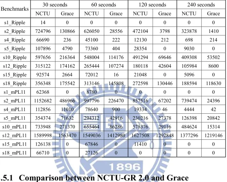
Table 2.1 Comparison total overflows between NCTU-GR 2.0 and Grace in a given time budget. ... 24

Table 2.2 Comparison the routing results between NCTU-GR 2.0 and Grace without time limitation... 26

Table 2.3 The usage of the proposed unilateral monotonic routing and HUM routing algorithms ... 27

Table 2.4 Comparison between congestion-aware box expansion scheme and tradtional scheme ... 28

Table 3.1 Design Information ... 43

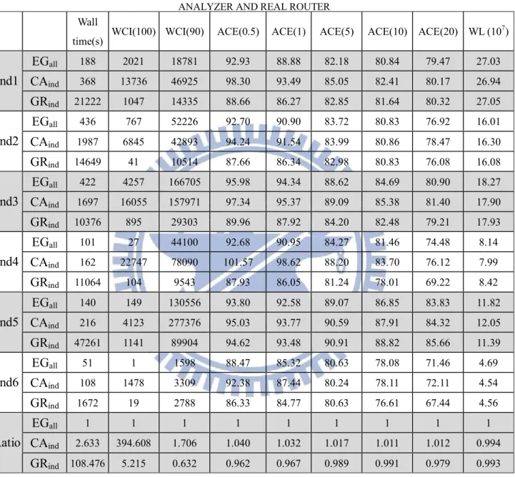
Table 3.2 Routing results comparison between E-Grace, industrial congestion analyzer and real router ... 44

Table 3.3 Design Information ... 45

Table 3.4 Different versions of E-Grace... 46

Table 3.5 Effectiveness of using relaxation-legalization method to handle the Scenic Constraint... 46

Table 3.6 Route Ind11 with different objectives ... 47

Table 3.7 Effectiveness of using throughput controlling method to trade off runtime and routing quality... 49

Table 3.8 Route Ind11 with extra blockages... 49

Table 4.1 Comparing the placement solutions in DAC12 contest based on the DAC12 metric, violations and TLMW... 57

Table 4.2 Benchmarks' information... 68

Table 4.3 Ropt with different features ... 69

Table 4.4 Global routing result comparison between NTUplace, Ropt1, Ropt2 and Ropt3... 70

Table 4.5 Detailed routing results of NTUplace ... 71

Table 4.6 Detailed routing result comparison between NTUplace, Ropt3, Ropt4, Ropt5 and Ropt6... 72

Table 4.7 Comparing Detailed routing results of mPL and Ropt6... 74

xii

Table 4.9 Comparing Detailed routing results of SimPLR and Ropt6... 75

Table 4.10 Comparison between the detailed routing results of the placement solutions in DAC12 contest... 75

Table 4.11 Comparison between Abacus and our legalizer ... 76

Table 5.1 Main features of modern global routers ... 79

Table 5.2 Net ordering methods comparision ... 93

Table 5.3 Routing result comparison between maze routing w/ and w/o bounding box and bounded-length maze routing ... 95

Table 5.4 Comparison of the routing result of H-BLMR-GR with and without RSMT-aware routing scheme ... 96

Table 5.5 Comparision of the routing result of global routers with heuristic-BLMR, Optimal-BLMR and [27] ... 97

Table 5.6 Comparison between NCTU-GR 2.0 and the other routers on overflow-free cases... 99

Table 5.7 Comparison between NCTU-GR 2.0 and the other routers on hard-to-route benchmarks ... 99

Table 6.1 Comparing NLA with previous layer assignment works on via count minimization problem ... 117

Table 6.2 The quality variations of NLA and [17] with different assignment ordering sequences ... 118

Table 6.3 The wirelength improvement and runtime of Post3DGR ... 119

Table 6.4 Comparing NCTU-3D-GR 2.0 with other 3D routers... 120

1

Chapter 1 Introduction

1.1 Overveiw of this Dissertation

With ceaseless advances in semiconductor technology shrinkage, the main contributing factors to the

increasingly more challenging routing problem include the high number of metal layers, wide range of

metal thickness, and complex design rules, thus routability has become a critical issue in VLSI physical

design flow. To address the routability issue, global routing plays an important role since global routing

bridges the gap between placement and detailed routing. In traditional physical design flow, the global

routing stage follows the placement stage to yield a rough routing result for most nets, and then the

detailed routing stage based on the rough routing result completes physical routes for every net and

finally realizes a detailed routing result. For example, Figs. 1.1(a), (b) and (c) respectively show a

placement solution, a global routing result and a detailed routing result for a design, in which the gray

rectangles denote macros, the small rectangles denote cells, and red circles denote pins of a net. Figure

1.1 illustrates that global routing identifies a set of routing regions that the net should pass through, and

detailed routing finds a physical routing path in these regions.

In this dissertation, a routability-driven placement and routing (P&R) flow (Fig. 1.2) is presented

based on the proposed global routing engines and post-placement routability optimizer. The proposed

global routing engines can not only cooperate with placers to obtain better routability placement Fig. 1.1 (a) A placement solution; (b) a global routing result; (c) a detailed routing result of a design.

2

solutions, but can also yield high-quality global routing results so that detailed routers can apply the

global routing results to generate good detailed routing results. Compared to the traditional placement

and routing flow, the flow shown in Fig. 1.2 pays more attention to the interaction between placement

and routing and optimizes the main factors to influence routability such like global congestion, local

congestion, wirelength and via count, which can detect and fix the congestion problems in the early

stages and thus contributes to faster design closure. The red boxes in Fig. 1.2 highlight the contributions

of this dissertation to deal with routability issue, introduced in the following four paragraphs.

To avoid wasting time on routing unroutable designs, a routing congestion estimator (RCE) can help

designers to fast judge whether a design is routable in the early stages to speed up the design closure.

Also, a RCE can cooperate with placers to optimize routability. Thus, this dissertation presents a

global-routing-based RCE cooperating with placers to improve routability. The proposed

global-routing-based RCE can offer more accurate routing congestion estimation than

probabilistic-based RCE [35, 36] since global-routing-based RCE can better capture the actual routing

behaviors. However, global-routing-based RCE is typically slower than probabilistic-based RCEs.

Because a RCE may be frequently launched in the placement stage, the placement stage would slow

down if the launched RCE is not fast enough. Accordingly, the objective of a global-routing-based RCE

is to identify an accurate congestion map as fast as possible. This dissertation presents an accurate and

fast global-routing-based RCE called Grace. In addition to testing Grace on academic benchmarks, we Fig. 1.2 Routability-driven placement and routing (P&R) flow.

3

also enhance Grace to fulfill industrial requirements and then apply the enhanced Grace in the industrial

design flow.

In the flow of Fig.1.2, RCE reports the congestion information of a placement solution to placers,

and then placers can move cells based on the congestion map to improve the placement solution's

routability. However, as cells move, the congestion map also changes, thereby degrading the

effectiveness to improve the routability of a placement. To resolve this problem, we develop a

routability optimizer Ropt that takes a placement solution and optimizes its routability by incremental

place-and-route. Ropt always maintains a global routing instance based on the current placement

solution. The global routing instance is built on a local-routability-aware model. Therefore, the global

routing instance provides both global and local congestion information to guide the placement

algorithms. Also, the placement algorithms in Ropt invoke a global routing engine to decide the placed

locations for movable cells.

After a placement solution is optimized by Ropt, the proposed global router NCTU-GR 2.0 is used

to identify a high-quality global routing result of the placement solution to provide a good blueprint for

detailed routing. Generally, the runtime of the detailed routing stage is hundred or thousand times of

that of the global routing stage. Good global routing results can diminish the time of detailed routing

and promote the final interconnection quality significantly. Because the routing quality of a global

routing result can be measured by the total overflow and total wirelength, minimizing overflows and

wirelength is the major task for global routing researches [3-21], where overflow means that a region's

routing demand exceeds its routing capacity. Compared to other state-of-the-art global routers [6, 11, 16,

17], the proposed NCTU-GR 2.0 can get global routing results with fewer overflows and shorter

wirelength. Note that, although Grace can be treated as a light global router, the algorithms used in

Grace and NCTU-GR 2.0 are largely different since their purposes are different. Chapter 5 will detail

the algorithmic differences between designing a global-routing-based RCE and a global router.

With semiconductor technology shrinkage, the number of metal layers ceaselessly increases. Thus,

4

planning for routing wires impacts the amount of vias, timing, and many manufacturing issues such like

antenna effect and double-vias. However, the typical global routing stage ignores these issues and

leaves these issues to detailed routing, which may make detailed routers struggle for these issues.

Accordingly, we develop a post-3D-global-routing tool Post3DGR between global routing and detailed

routing to refine a given 3D global routing result, which can ease the effort of detailed routers to speed

up the design closure. The proposed Post3DGR can reduce the vias, congestion, and wirelength of a

given 3D global routing result by re-routing nets and re-planning wires' layers. With some modifications,

Post3DGR also can take antenna effect into account.

The rest of this dissertation is organized as follows. Chapter 1 introduces the problem formulation

and background of global routing. Chapter 2 presents a fast global-routing-based RCE called Grace

whose goal is to identify a satisfactory global routing result to predict routing congestion as fast as

possible. Chapter 3 presents an enhanced Grace applied in the industrial flow to consider timing and

local congestion, and target congestion ratio. Chapters 4 introduces the proposed incremental

place-and-route tool Ropt that can optimize the routability of a given placement solution. Chapter 5

presents a global router called NCTU-GR 2.0 whose objective is to obtain high-quality global routing

results in a reasonable runtime to guide detailed routers. A post-3D-global-routing tool Post3DGR is

detailed in Chapter 5. Finally, Chapter 7 draws conclusions.

1.2 Background

In global routing problem, typically the given placement solution is partitioned into a 3-dimension

(3D) array of global cells (Fig. 1.3(a)), and then the array of global cells is modeled to a 3D grid graph

(Fig. 1.3(b)). Generally, there are two strategies to deal with global routing problem on the 3D grid

graph. One directly performs global routing on a 3D grid graph [3-6]. Although directly performing

global routing on a 3D grid graph may achieve a better result, it is time-consuming. Thus, the

mainstream approach is to condense 3D grid graph into 2D grid graph first, and then peform 2D global

5

routing wire to the corresponding metal layers to obtain a 3D global routing result [7-21]. Figure 1.3(c)

shows the general flow adopted in most global routers to tackle 3D global routing porblem, the

functions of each stage are detailed in the follows.

1.2.1 Building Grid Graph and the Objectives of Global Routing

In the grid graph, each grid node refers to a global cell (G-cell), and each grid edge corresponds to a

boundary between two abutting global cells in the same layer. Meanwhile, each via edge connects two

abutting G-cells in two adjacent layers. The number of routing tracks that can be accommodated across

the abutting boundary is defined as the capacity c(e) of a grid edge e, and the number of wires that pass

through grid edge e is called grid edge’s demand d(e). The overflow of a grid edge e is defined

max(d(e)-c(e), 0), the total overflow is the sum of overflows on all grid edges, and the maximum

overflow is the maximum overflow among all edges. For simplicity, the capacity of each via edge is not

limited, which is also adopted in most of global routing researches [3-21]. Given the pins' locations of

each net distributed on the grid graph, the objective of global routing problem is to identify a highly

routable global path to connect the pins of each net. The quality of a global routing result is generally

measured by the total overflow and wirelength.

Figure 1.4 shows how to compute the capacity of 2D grid edges in the mainstream flow of 2D global Fig. 1.3 (a) partition a placement into a 3D array of G-cells; (b) model the 3D array of G-cells into a grid graph; (c) typical global routing flow.

6

routing with layer assignment, in which the numbers next to 3D grid edges denote the capacity of the

3D edges. After the 3D grid graph is compacted to a 2D graph, the capacity of a 2D grid edge is

obtained by adding up the capacities of its corresponding 3D grid edges.

1.2.2 Net Decomposition

Most global routers decompose each multi-pin net into two-pin subnets, because net decomposition

can simplify a multi-terminal routing problem to a two-terminal routing problem. Before routing stages,

the rectilinear Steiner minimal tree (RSMT) or rectilinear minimum spanning tree (RMST) construction

algorithms are commonly used to generate the initial topology for each multi-pin net and then each

multi-pin net is decomposed into two-pin subnets based on its topology. For example, Figs. 1.5(a) and

1.5(b) show the initial topologies of a four-pin net generated by RSMT and RMST, respectively, in

which the green rectangle denotes a Steiner point, and the topologies of the four-pin net in Figs. 1.5(a)

and 1.5(b) can be decomposed to 4 and 3 two-pin subnets, respectively. Because a RSMT has shorter

wire length than a RMST has, net decomposition by RSMT is popular in many literature. FLUTE [23]

is a very fast and accurate RSMT construction tool, which is widely used by many modern global

routers. FLUTE not only quickly constructs a good RSMT for a multi-pin net, but also obtains optimal

RSMTs for nets with nine or fewer pins. However, FGR [3] indicates that the RSMT has less routing

10

0

5

1

0

10

15

11

7

flexibility than the RMST as it owns Steiner points and generates more flat segments than the RMST,

and the used data structure of RSMTs is more complex than that of RMSTs. On the contrary, the RMST

can simply complete each subnet’s routing with pattern routing or monotonic routing to avoid

congestion regions. Consider wirelength and routing flexibility, in which a RMST that encourages

multiple two-pin routings to merge together with multiple paths that pass through the same grid edges

(Fig. 1.5(c)). This ideal solution avoids passing through congested regions by using a shorter total wire

length than that of a RMST that does not encourage finding joint wires. However, how to identify a

RMST with joint wires is a challenge.

1.2.3 Pattern Routing and Monotonic Routing

Pattern routing adopts specific routing patterns to connect two pins. The most common patterns are

L-shaped or Z-shaped. The main advantage of pattern routing is that it can complete the path searching

in a very short time, but its solution space is very tiny. To mitigate the huge performance gap between

pattern routing and maze routing, Pan et al. [14] present monotonic routing to enrich the solution space.

Monotonic routing uses the dynamic-programming technique to identify a routing path from the source

to the target without any detour. The time complexity of monotonic routing in a m  n grid graph is

O(mn), which is the same as that of the Z-shaped pattern routing.

1.2.4 Negotiation-based Rip-up and Rerouting (NRR)

Rip-up and re-routing technique is widely used in global and detailed routing. Given an illegal Fig. 1.5. Four-pin net decomposition by (a) RSMT; (b) RMST; (c) RMST with a joint wire, subnets n1 and n2 share a joint wire.

8

routing solution, rip-up and rerouting technique iteratively removes the nets with violations and reroutes

them sequentially to expel violations. In global routing problem, a violation occurs when an overflow is

produced. Widely, the negotiation technique, as proposed in PathFinder [22], is associated with rip-up

and re-routing technique (NRR) in modern global routers to improve the ability of overflow removal.

The main idea of NRR is to increase the penalty of a grid edge at current iteration that overflowed at the

previous iteration. Thus, path searching intends to avoid passing previously overflowed grid edges. [22]

formulates the negotiation-based routing cost of grid edges e as follows,

e e e

e b h p

c (  ) , (1.1)

where ce represents the routing cost of e; be denotes the base cost; he denotes the history cost, and pe

denotes the congestion penalty. The history cost he increases as overflow occurs. The value of he in the

(k+1)-th iteration is given by:

     _   otherwise overflowed is if 1 k e inc k e k e h e h h h , (1.2)

where h1e1, hinc is a constant, and hek is updated in every iteration. In addition, FGR [3] presents

another formula to preserve the base cost as follows.

e e e

e b h p

c    . (1.3)

Several variations of negotiation-based cost functions have been discussed in [10-12, 16-17].

1.2.5 Layer Assignment

The goal of layer assignment in global routing is to translate a 2D global routing result into a 3D

result on minimizing the number of vias while not changing routing topology or increasing any

overflows, which is called the congestion-constraint layer assignment problem. Congestion-constrained

layer assignment problem for via minimization has been proven to be NP-complete [34] and extensively

studied. BoxRouter2.0 [9] adopted integer linear programming to minimize via count minimization.

FGR [3] greedily assigned net edges to the corresponding metal layers by heuristics. Lee et al. proposed

9

order at first and then assigning each net to the appropriate layer by a dynamic-programming technique.

FastRoute 4.0 [16] decomposes multi-pin nets to two-pin net, then using the dynamic-programming

algorithm to assign each two-pin net one bye one. Dai et al. [17] presented a congestion-relaxed layer

assignment with a layer shifting algorithm, followed by net rip-up and re-assigning to further reduce the

number of vias. In addition, some researchers extended the layer assignment problem to consider via

overflow [28-29], double patterning [30], timing [31], and antenna effect [32-33].

1.2.6 Comparison of Recent Global Routers

Table 1.1 lists the well-know global routers developed in recent six years. Although most global

routers in Table 1.1 are based on the global routing flow shown in Fig. 1.3(c), they have different

opinions on several issues. Table 1.2 shows the issues that are widely discussed in recent global routing

researches. For instance, the routers in [3, 7, 71] use RMST to be the initial tree topology for each net,

while the routers in [16, 71] use RSMT; NTHU-Route [11] reroutes the nets in the un-congested region

earlier, while the routers in [3, 12, 17] reroutes the nets in the congested region earlier; Box-Router [9,

70] rips-up a set of nets and then reroutes these nets one by one, while the routers in [4, 7, 11, 17] rip-up

a net and then reroute it immediately. On the parallel routing issues, GRIP [4, 5] parallelize global

routing on a cluster computing environment, NCTU-GR [18, 71] performs on a many-core server, the

router in [19] performs on a GPU-CPU hybrid platform.

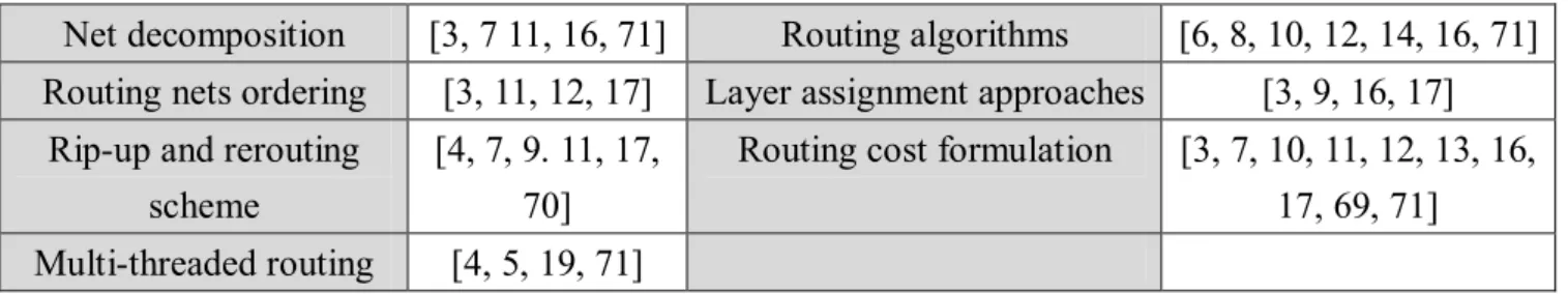
Net decomposition [3, 7 11, 16, 71] Routing algorithms [6, 8, 10, 12, 14, 16, 71] Routing nets ordering [3, 11, 12, 17] Layer assignment approaches [3, 9, 16, 17]

Rip-up and rerouting scheme

[4, 7, 9. 11, 17, 70]

Routing cost formulation [3, 7, 10, 11, 12, 13, 16, 17, 69, 71] Multi-threaded routing [4, 5, 19, 71]

TABLE 1.2 THE ISSUES DISCCUSED IN RECENT GLOBAL ROUTING RESEARCHES

NTHU-Route [69, 11] FastRoute [13-16] FGR [3, 7] MGR [6]

NTUgr [12] Box-Router 2.0 [70, 9] NCTU-GR [17, 18, 71] Archer [10]

GRIP [4, 5] HybridGR [19] Maize-Router [8]

10

Chapter 2 Grace: A Fast Global-routng-based

Routing Congestion Estimator

2.1 Introduction

Routability is of primary concern in nanometer-scale design. Considering the routability issue in

placement stage can avoid generating an unroutable design. Two strategies are generally adopted by

routability-driven placement to estimate the congested regions (hot spots). First, the probabilistic

method estimates the routing congestion of a region by using the pin density and the nets’ bounding box

or Steiner tree [35, 36]. Although fast, this method typically fails to capture actual routing behavior, and

therefore has low estimation accuracy. The second congestion estimation strategy performs global

routing to analyze routing congestion [37]. The latter method can identify more precisely the congestion

information. However, such an approach is markedly slower than the former one. Among the modern

routability-driven placers, Ripple [38], NTUplace [39] and the placers in [40, 41] used the former

strategy, whereas SimPLR [42], IPR [43], CRISP [44] and GRplacer [45] adopted the latter one. Clearly,

it is inevitable to trade-off routing quality for better run-time performance when these built-in global

routers are concerned.

Maze routing with A* search scheme is the indispensable kernel algorithm of state-of-the-art global

routers [3-19]. For hard-to-route benchmarks, these routers attempt to eliminate overflows by iteratively

ripping up and rerouting overflowed nets by using maze routing. However, maze routing is slower than

other routing algorithms, such as pattern routing and monotonic routing algorithms. Several works have

attempted to reduce runtime by developing alternative routing algorithms in order to lower the

frequency of invoking maze routing. For instance, Archer [10] developed the U-shaped pattern routing

algorithm; NTUgr [12] presented the escaping routing algorithm; and FastRoute 4.0 [16] developed the

3-bend routing algorithm. These routing algorithms run faster than maze routing within a quite limited

11

identify better routes. Consequently, maze routing still consumes the majority of the runtime in the

entire routing flow.

This work presents an extremely fast global router called Grace, which does not include maze

routing to achieve high speedup as an ideal built-in routing congestion estimator for placers.

(a) This work presents two efficient routing algorithms, called unilateral monotonic routing and

hybrid unilateral monotonic (HUM) routing. HUM routing can identify a better routing path than

U-shaped pattern routing, 3-bend routing, and escaping routing. Moreover, the time complexity of

HUM routing is the same as those of these three approaches, linear in terms of the size of the

routing region.

(b) Many routers adopt bounding boxes to limit the searching region of routing. Consequently, the

bounding box size affects the routing quality and runtime. This work presents an efficient

congestion-aware bounding box expansion scheme. With this scheme, the proposed router can

improve runtime by 50% than without this scheme.

(c) The proposed router relies on HUM routing to eliminate overflows without invoking maze routing.

Experimental results indicate that the proposed router achieves a routing quality similar to that of

the proposed maze-routing-based router NCTU-GR 2.0 [18]. Moreover, the run-times of the

proposed router are up to 26 times faster than those of [18] on large benchmarks.

The rest of this chapter is organized as follows. Section 2 introduces the global routing problem and

the research objective. Section 3 then presents the proposed unilateral monotonic routing, HUM routing

algorithms and a congestion-aware bounding box expansion scheme. Section 4 displays the design flow

of the proposed global router. Section 5 summarizes the experimental results. Conclusions are finally

drawn in Section 6.

2.2 Problem Description

Global routing is formulated as the routing problem on a grid graph G(V, E) , where V denotes the set

12

related G-cells to its two end nodes. The capacity c(e) of a grid edge e indicates the number of routing

tracks that can legally cross the abutting boundary. The number of wires that pass through grid edge e is

called the demand of the grid edge d(e). The overflow of a grid edge e is defined as follows. The total

overflow is the sum of overflows on all edges of E.

otherwise e c e d if s w e c e d e overflow L L , ) ( ) ( , 0 ) ( * )) ( ) ( ( ) (        (2.1)

where wL and sL respectively denote the minimum wire width and wire spacing at layer L where e

belongs. In modern designs, higher layers have larger wire width and wire spacing.

Conventionally, overflow and wirelength minimizations have a higher priority than runtime

improvement for global routing that offers a global path to guide the detailed routing of each net.

However, when global router plays the role as a congestion estimator, the runtime issue become more

critical because the estimator have to report the congestion information to placers in a limited time

budget (e.g. around 1~5 min). Accordingly, this work focuses on comply with the limited time budget to

complete global routing.

2.3 The Proposed Algorithms for Accelerating Routing

Although capable of identifying a detour-free path efficiently, monotonic routing fails to replace

maze routing when a detoured path is required to avoid obstacles or congested regions. A detour is

viewed as a move away from the target. To approach the behavior of maze routing, we develop an Fig. 2.1. (a) Vertically monotonic routing path; (b) horizontally monotonic routing path; (c) routing path combining vertically and horizontally monotonic routing.

13

extremely fast routing algorithm, called unilateral monotonic routing, capable of seeking a detoured

path and running in the same time complexity as that of monotonic routing. Unilateral monotonic

routing identifies a least-cost routing path within a limited region using minimal horizontal or vertical

distance. Two unilateral monotonic routing types are defined as follows.

Definition. Horizontally/Vertically monotonic (HM/VM) routing identifies the least-cost routing path

from the source to the target using minimal horizontal/vertical distance.

For a HM/VM routing path, a detour occurs only in vertical/horizontal move. Figures 2.1(a) and

2.1(b) illustrate a VM routing path and a HM routing path, respectively, in which the gray rectangles

represent congested regions. Although the solution space of HM or VM routing is less than that of maze

routing, alternatively invoking HM and VM routings together can increase the solution space

significantly. Figure 2.1(c) depicts an example of invoking successive HM and VM routings, the path in

Fig. 2.1(c) consists of a HM routing path from s to an internal node u and a VM routing path from t to u.

2.3.1 Unilateral Monotonic Routing

Without a loss of generality, the proposed unilateral monotonic routing is introduced by using an

example of VM routing shown in Fig. 2.2. At the beginning of VM routing, the congestion map (Fig.

2.2(a)) is formulated into the global routing model (Fig. 2.2(b)), and the congestions is formulated into

the routing cost on each grid edge, then a window is given to enclose the source and target with the

height of vertical distance between the source and target and the width of horizontal distance larger than

that between the source and target (Fig. 2.2(b)). The window size determines the runtime and the

routing quality of the unilateral monotonic routing. Section 3.3 in this chapter will introduce how to

determine the window size. Figure 2.3 shows the pseudo code of the VM routing algorithm, in which

source s and target t are located at (x1, y1) and (x2, y2) respectively; B.l and B.r represent the left and

right borders of windows B, respectively; cost(v, u) denotes the routing cost of grid edge e(v, u); d(u)

refers to the least cost of the VM routing path within B from s to u; and π(u) is the predecessor of u. The

14

bottom row, i.e. the row where the start node belongs. The second stage computes the d(u) values of

nodes in all rows, except for the bottom row, from the row above the bottom row to the top one. The

first stage is a simple sequential examination initiating from the start node towards the left and right

boundaries of B, and then the second stage processes all rows except for the bottom one sequentially

and upwards. In the second stage, based on the dynamic programming algorithm, a two-phase flow is

developed and the d(u) value of each node is computed row by row. The first phase determines the Fig. 2.2. Example of VM routing. (a) a congestion map; (b) the routing model of (a), the dotted lines denote the grid edges; (c) The predecessor of each node u in the row of y-coordinate y1 after d(u) is obtained, the arrow of each node denotes its predecessor; (d) the predecessor of each node u in the row of y-coordinate y1+1 after lclb(u) is obtained; (e) the predecessor of each node u in the row of

y-coordinate y1+1 after d(u) is obtained; (f) the routing result of VM routing.

(c) (d)

(e) (f)

(a) (a) (b)

15

least-cost VM path to connect every node from the start node at the left or bottom side, while the second

phase determines the least-cost VM path to connect every node from the start node at the right side. By

the two-phase operation, the least-cost VM path to reach every node within B from the start node is then

identified.

Upon commencement of the second stage, the d(v) value of each node v∈(i,y1) for B.liB.r is identified. By assuming that node u is located at (i, y1+1), lclb(u) is the least of all costs of the VM

Algorithm Vertically monotonic routing

Input: source s(x

, y

), target t(x

, y

), bounding box B, cost array d

2. for x= x1-1 to B.l

3. u=(x, y1), v=(x+1, y1);

4. d(u)= d(v)+ cost(v, u), π(u)= v; 5. end for

6. for x= x1+1 to B.r

7. u=(x, y1), v=(x-1, y1);

8. d(u)= d(v)+ cost(v, u), π(u)= v; 9. end for

10. for y= y1+1 to y2

11. u=( B.l , y), v=( B.l, y-1)

12. lclb(u)= d(v)+ cost(v, u), π(u)= v 13. for x= B.l +1 to B.r

14. u=(x, y), v1=(x-1, y), v2=(x, y-1);

15. if lclb(v1) + cost(v1, u) < d(v2) + cost(v2, u) 16. lclb(u)= lclb(v1)+ cost(v1, u), π(u)= v1

17. else

18. lclb(u)= d(v2)+ cost(v2, u), π(u)= v2 19. end for

20. u=( B.r , y), d(u) = lclb(u) 21. for x= B.r -1 to B.l

22. u=(x, y), v3=(x+1, y), d(u) = lclb(u) 23. if d(v3) + cost(v3, u) < d(u)

24. d(u) = d(v3) + cost(v3, u), π(u)= v3 25. end for

26. end for

16

routing paths from s to u when the predecessor of u is at its left or bottom side, and can be obtained via

the following equation in the first phase,

       otherwise )), , ( ) ( ), , ( ) ( min( of boundary left on the is if ), , ( ) ( 2 2 1 1 2 2 u v cost v d u v cost v lc B u u v cost v d ) u ( lc lb lb (2.2)

where v1 and v2 represent the left and bottom adjacent nodes of u, respectively. During the second phase,

the least cost of VM paths to reach node u from the start node at the right side (denoted by lcr(u)) and

then the least-cost VM path to reach node u from the start node are determined sequentially by the

following equation.       otherwise )), , ( ) ( , min( of boundary right on the is if 3 3 cost v u v d ) u ( lc ) u ( lc B u ), u ( lc ) u ( d r lb lb (2.3)

where v3 represents the right adjacent node of u. If u is on the right boundary of B, the predecessor of u

must be on the left side or on the bottom side of u; thus d(u) equals lclb(u). While each node u is

examined sequentially from right to left in the second phase, the least-cost VM path to reach each node

from the start node is then determined by Eq. (2.3).

In Fig. 2.3, lines 1 to 9 calculate the least cost of the VM paths from s to each node v(i,y1) for

B.liB.r (Fig. 2.2(c)). Next, based on the dynamic programming method, the least-cost VM path from

s to each node of each row within B is identified from the row of y-coordinate y1+1 to the row of

y-coordinate y2, (lines 10 to 26), where lines 11 to 19 identify the values of lclb(u) by Eq. (2.2) and lines

20 to 25 identify the values of d(u) by Eq. (2.3). Figure 2.2(d) shows the predecessor of each node u in

the s-to-u path of lclb(u) in the row of y-coordinate y1+1. Meanwhile, Fig. 2.2(e) shows the predecessor

of each node u in the s-to-u path of d(u) in the row of y-coordinate y1+1. Upon completion of the VM

routing, each node within B has a least-cost VM path to reach s along its predecessor (Fig. 2.2(f)).

Therefore, the least-cost VM path from s to t is also identified. Obviously, the time complexity of

17

2.3.2 Hybrid Unilateral Monotonic Routing

Compared to maze routing, unilateral monotonic routing still offers a limited solution space to solve

overflows. This section introduces a hybrid unilateral monotonic (HUM) routing algorithm to search for

larger solution space than unilateral monotonic routing offers. The HUM routing concept assumes that

each node within B can be an intermediate point connecting the start and target nodes. The HUM path

consists of two paths, i.e. the path linking the start node with an intermediate point and the path linking

the intermediate point with the target node. Each path can be formed by unilateral monotonic routing.

Since a path can be formed by VM or HM routing, four combinations are available to form a HUM

routing path. By assuming that bounding box B encloses nodes u and v, VMPB(u,v) and HMPB(u,v)

represent a VM routing path and a HM routing path connecting u with v within B, respectively. A HUM

routing path connecting s with t belongs to one of the following four path types: (VMPB(s,u), VMPB(u,t)),

(VMPB(s,u), HMPB(u,t)), (HMPB(s,u), VMPB(u,t)) and (HMPB(s,u), HMPB(u,t)) for each node u within B.

Whereas (VMPB(s,u), VMPB(u,t)) denotes a path concatenation operation that combines two unilateral Fig. 2.4. The pseudo code of hybrid unilateral monotonic routing algorithm.

Algorithm Hybrid Unilateral Monotonic Routing

Input: source node s, target node t, bounding box B

1. Initialize cost array Aryvs, Aryvs, Aryhs, Aryht 2. //Find the paths from each node in B to s

3. Vertically_Monotonic_Routing(s, B.bl, B, Aryvs) 4. Vertically_Monotonic_Routing(s, B.tr, B, Aryvs) 5. Horizontally_ Monotonic_Routing(s, B.bl, B, Aryhs) 6. Horizontally_Monotonic_Routing(s, B.tr, B, Aryhs) 7. //Find the paths from each node in B to t

8. Vertically_Monotonic_Routing(t, B.bl, B, Aryvt) 9. Vertically_Monotonic_Routing(t, B.tr, B, Aryvt) 10. Horizontally_ Monotonic_Routing(t, B.bl, B, Aryht) 11. Horizontally_ Monotonic_Routing(t, B.tr, B, Aryht) 12. foreach node u in B

13. mrc(u)=min(Aryhs(u), Aryvs(u))+min(Aryht(u), Aryvt(u)) 14. end foreach

18

monotonic paths of one or two type to form a HUM path linking start and end nodes. Figure 2.4 shows

the proposed HUM routing algorithm. The least costs of VMPB(s,u), VMPB(t,u), HMPB(s,u) and HMPB(t,u) of

each node are stored in the arrays Aryvs, Aryvt, Aryhs and Aryht, respectively, while B.bl and B.tr

represent the nodes at the bottom-left and top-right corners of B, respectively. Lines 3 – 6 regard s as the

start node, and B.bl and B.tr as pseudo targets. Then, lines 3 and 4 invoking VM routing from s to the

pseudo targets obtain VM routing paths from s to every node within B; lines 5 and 6 invoking HM

routing from s to the pseudo targets obtain HM routing paths from s to every node within B. Similarly,

lines 8 – 11 regard t as the start node and B.bl and B.tr as the pseudo targets, and then obtain VM

routing paths and HM routing paths from t to every node within B. Accordingly, lines 2 – 11 identify

the value of each element in Aryvs, Aryvt, Aryhs and Aryht. Thereafter, the least costs of VMPB(s,u),

VMPB(t,u), HMPB(s,u) and HMPB(t,u) for each node u within B are obtained (Fig. 2.5(a)-(d)). The algorithm

then selects the least-cost HUM routing path among the candidates of four path types (lines 12 – 15).

Fig. 2.5. Four path types in B with congested regions (gray rectangles). (a) VMPB(s,u), (b) VMPB(t,u), (c) HMPB(s,u), and (d) HMPB(t,u).

(a) (b)

19

The time complexities of three parts, lines 2-11, lines 12-14 and line 15 are all O(|B|).

Correspondingly, the time complexity of HUM routing algorithm is still O(|B|), which is faster than that

of maze routing with A* search scheme (O(|B|log|B|)). Figure 2.6 compares the proposed HUM routing

with 3-bend routing and escaping routing, indicating that the time complexities of 3-bend routing and

escaping routing are also O(|B|). Figures 2.6(a) and 2.6(b) summarize the routing results of 3-bend

routing and escaping routing with two overflows and with an overflow, respectively. In contrast, the

proposed HUM routing algorithm can identify an overflow-free path (Fig. 2.6(c)) with the pattern

(HMPB(s,u), HMPB(u,t)). Notably, even if HUM routing cannot identify an overflow-free path, it can

always identify a least-cost HUM path which must cost less than or equal to that of 3-bend routing and

escaping routing. Because, the solution space of HUM routing totally covers and is much larger than

that of 3-bend routing and escaping routing.

Assume that most of overflowed grid edges within B are aligned in a row similar to the congestion

map in Fig. 2.1(a), the least costs of HMPB(s,u) and HMPB(u,t) are likely larger than the least costs of

VMPB(s,u) and VMPB(u,t). Therefore, the operations of exploring HMPB(s,u) and HMPB(u,t) can be regarded

as redundant and are thus omitted. Based on this observation, four HUM routing types are explored only

once for every net at the first time when it is routed by HUM routing. If a net is rerouted by HUM

routing in the later routing stage, only the HUM routing type that initially identified the least-cost path (a) (b) (c)

Fig. 2.6. (a) Routing result of 3-bend routing with two overflows; (b) routing result of escaping routing with an overflow; (c) routing result of the proposed HUM routing without overflows.

20

is invoked. By this scheme, experimental results indicate that similar routing quality and an

approximately 23% decrease in runtime of HUM routing can be achieved.

2.3.3 Congestion-aware Bounding Box Expansion

Bounding box is widely adopted to limit the searching region of routing. In conventional global

routers, the initial bounding box is slightly larger than the minimum rectangle enclosing the terminals of

the routed net. The inability to identify an overflow-free path within the bounding box causes the

bounding box to expand and, then, the overflowed net is rerouted again. The box expansion policy

based on current congestion information has seldom been discussed in the literature. The traditional box

expansion scheme tends to over-expand, subsequently increasing the runtime. For instance, Fig. 2.7(a)

shows a routing path with a vertical overflowed edge. Traditional box expansion chooses to expand the

bounding box along both x and y coordinates to resolve the overflow. However, the bounding box only Fig. 2.7. Example of congestion-aware bounding box expansion. (a) Routing path with an vertical overflow; (b) the overflow map of the benchmark superblue1 after the initial routing; (c) currently identified path Ps,t and path Ls,t that is expected to be across the left side of the bounding box; (d) the estimated lower bound cost of Ls,t is the sum of the costs of Ps,v and Pt,u plus manh(v, u)* α.

(a) (b)

21

needs to expand horizontally in Fig. 2.7(a) while the vertical expansion is unnecessary. Figure 2.7(b)

displays the congestion map of the benchmark superblue1 after the initial routing. The red regions

represent the overflowed grid edges, which normally range horizontally or vertically, implying that the

situation in Fig. 2.7(a) occurs frequently during routing. Based on this observation, this work presents a

novel congestion-aware bounding box expansion scheme to avoid over expanding.

Before rerouting a net, this work analyzes the amount of horizontal overflowed grid edges (HOEs)

and vertical overflowed grid edges (VOEs) by tracing the routing path of the rerouted net. If the number

of HOEs is more than that of VOEs, the bounding box expands vertically by δ units; on the contrary, the

bounding box expands horizontally. If a tie occurs, the bounding box randomly chooses to expand

horizontally or vertically. Single-direction expansion can restrict the sizes of bounding boxes to reduce

the runtime. In our implement, the initial bounding box is set as the minimum rectangle enclosing two

terminals to be routed, and δ is set to 5+30/ri, where ri denotes the rip-up and rerouting times of the

rerouted net. Moreover, based on the assumption that two opposite sides have different congestion

states, extending the side near the congested region may be unnecessary, implying that the extension of

each boundary of B should be discussed separately. The algorithm examines each boundary side of B to

determine the necessity of box boundary expansion at the end of HUM routing. Without a loss of

generality, the left boundary of B is used to illustrate the concept. Left boundary expansion can be

regarded to have the intention to find a path Ls,t on the left side of B; in addition, Ls,t has a lower routing

cost than that of the currently identified path Ps,t (Fig. 2.7(c)). Namely, a situation in which the routing

cost of Ps,t is lower than the least cost of Ls,t implies that the left boundary expansion is unnecessary.

However, the least cost of Ls,t is unknown because the region on the left side of B has not been explored

yet. Thus, the estimated lower-bound cost of Ls,t, ecL, is defined by the following equation to evaluate

the necessity of boundary expansion. If the currently identified path Ps,t costs less than ecL, the left

boundary remains unchanged at the next expansion of B.

)

)

(

)

(

)

(

(











min

d

s,v

d

t

,

u

manh

v

,

u

ec

22

where VL denotes the set of grid nodes on the left boundary of B; d(s,v) and d(t,u) represent the least

cost of the unilateral monotonic routing paths from s to v and from t to u, respectively; manh(v,u) refers

to the Manhattan distance between v and u; and α is the lower-bound routing cost of a grid edge. In this

work, α is set to 1. Notably, d(s,v) and d(t,u) are known values that have been computed by the HUM

routing (Fig. 2.7(d)). With this, before a net ni is rerouted, the path of ni is first traced to obtain HOEs

and VOEs. If the number of VOEs is more than that of HOEs, extending the left and right boundaries of

the bounding box B of ni is considered. If ni is not routed by HUM routing in previous routing, the left

and right boundaries of B extend immediately. Otherwise, the decision of boundary expansion is made

according to the previous discussion.

2.4 Design Flow of Grace

Figure 2.8 shows the design flow of the proposed routing congestion estimator Grace. First, the

multi-layer routing region is projected on a 2D plan and each net is decomposed into two-pin nets based

on the topology of the RMST because the works in [1, 7, 18] indicate that RMST offers better flexibility

than Steiner tree to avoid blockages or congestion. An initial congestion graph is then generated by

pattern routing and monotonic routing. Next, the rip-up and rerouting stage iteratively reroutes the

overflowed net until an overflow-free routing result is obtained or the runtime exceeds the given time

budget. In the rip-up and rerouting stage, before net ni is rerouted, the bounding box of ni is expanded Fig. 2.8. Design flow of Grace

23

according to the proposed congestion-aware expansion scheme. For a situation in which the width of the

bounding box is equal to the x-distance between the source and the target of ni, ni is rerouted using HM

routing. Moreover, if the height of the bounding box is equal to the y-distance between the source and

the target of ni, ni is rerouted using VM routing. Otherwise, ni is rerouted by HUM routing.

2.5 Experimental Results

The proposed algorithms are implemented in C/C++ language on a quad-core 2.4 GHz Intel

Xeon-based linux server with a 50GB memory (only a single core is used). By hosting a

routability-driven placement contest, ISPD11 has motivated many researchers to develop effective

modern placers [38, 39, 42]. Ripple [38] and mPL11 placed first in the contest; their contest placement

results are adopted here as the input benchmarks in our experiments. We compare Grace with

NCTU-GR 2.0 [18] which is one of the fastest global routers. The experiments in [18] indicate that

NCTU-GR 2.0 runs 1.90X, 1.77X and 18.66X faster than NTHU-Route 2.0 [11], FastRoute 4.1 [16],

and NTUgr [12], respectively. In addition, in the old benchmarks [1, 2], the minimum wire spacing and

width are uniform and all pins locate at the lowest layer. In contrast, in new benchmarks [46] used in

this work, the minimum wire spacing and width of different layers are different and pins may locate at

high layers. Because most of traditional routers do not consider these new features, we cannot directly

adopt them to route the new benchmarks. However, recent routers NCTU-GR 2.0, BFG-R [7] and

CGRIP [35] can handle these new features, but the runtime of BFG-R and CGRIP is much larger than

NCTU-GR 2.0. Owing to its robustness and efficiency, the routability-driven placement contest in

DAC12 [47] and ICCAD12 [48] selects NCTU-GR 2.0 to be the evaluation tool. In the following

experiments, NCTU-GR 2.0 and Grace perform on the same machine. Notably, NCTU-GR 2.0 has the

parameters of via cost, wirelength optimization level, pattern routing iteration, monotonic routing

iteration and post routing iteration, which are set to 1, 50, 2, 2 and 0, respectively. The setting of the