數種新型多天線系統分析方法

(1)

國

立

交

通

大

學

電信工程學系

碩

士

論

文

數種新型多天線系統分析方法

Several New Analysis Strategies of Multiple Antenna Systems

研究生：莊瑞廷

(Jui-Ting Chuang)

指導教授：陳富強博士 (Dr. Fu-Chiarng Chen)

(2)

數種新型多天線系統分析方法

Several New Analysis Strategies of Multiple Antenna Systems

研究生：莊瑞廷 Student：Jui-Ting Chuang

指導教授：陳富強博士 Advisor：Dr. Fu-Chiarng Chen

國立交通大學

電信工程學系

碩士論文

A Thesis

Submitted to Department of Communication Engineering

College of Electrical Engineering and Computer Science

National Chiao Tung University

in partial Fulfillment of the Requirements

for the Degree of

Master of Science

in

Communication Engineering

Aug 2008

Hsinchu, Taiwan, Republic of China

(3)

I

數種新型多天線系統分析方法

學生：莊瑞廷指導教授：陳富強博

士

國立交通大學電信工程學系碩士班

摘要

在本論文中，我們研究了兩組評估多天線系統效能的電磁分析。第一項是輻射效率 (Radiation Efficiency) 的綜合分析，第二項是新型天線空間相關係數 (Antenna Spatial Correlation)的計算方法。論文中所有的個案討論都將以偶極天線做分析基準。

首先，我們綜合分析了一個全主動反射系數 (Total Active Reflection Coefficient,TARC) 和輻射效率的表示方式。利用矩陣特徵值分解 (Eigenvalue Decomposition (EVD))可將 TARC 表示成天線反射功率矩陣特徵值的組合。我們利用此方法計算反射係數和輻射效率的最大值和最小值,並分析反射係數和輻射效率的特性如何隨著天線埠饋入不同相位訊號時有所改變,我們也分析不同天線匹配網路如何影響此反射系數和輻射效率。

最後我們提出兩組適用於任意大角度分佈入射角度 (Large Angular Spread Angle-of-Arrival)的相關係數近似公式。利用此兩組公式，我們進一步計算含天線偶合效應的相關係數。基於此兩組近似公式的計算方法不僅可以有效降低計算複雜度，在精確度上也有不錯的表現。

(4)

II

Several New Analysis Strategies of Multiple Antenna

Systems

Student: Jui-Ting Chuang Advisor: Dr. Fu-Chiarng Chen

Department of Communication Engineering

National Chiao Tung University

Abstract

In the thesis, we focus on two electromagnetic analysis strategies to evaluate the performance of multiple antenna systems. The first is composite analysis of radiation efficiency. The second is a new calculation method of antenna spatial correlation. All case studies are simulated using dipole antennas.

First a composite analysis on total active reflection coefficient (TARC) and radiation efficiency are conducted.They can be described as the eigenvalues combination of antenna reflection power matrix utilizing eigenvalue decomposition (EVD).We not only evaluate the maximum and minimum value of TARC and radiation efficiency,but also their changes in characteristics when the antenna ports excite signals with different phases.Furthermore the investigations on how antenna termination networks influence TARC and radiation efficiency are also analyzed .

We further propose two new approximate antenna spatial correlation formulations which are suitable for arbitrary large angular spread angle of arrival (AoA) distribution. By using these two formulations, we further calculate spatial correlation incorporating antenna mutual coupling. Time complexity can be reduced and it still maintain good accuracy by utilizing the calculating method based on these two approximate formulations.

(5)

III

Acknowledgements

I would like to express my sincere gratitude to my advisor, Dr. Fu-Chiarng Chen for his valuable suggestions, guidance, and inspiration. Without his advice, it is impossible for me to complete this research. Sincere thankfulness is also given to my elder fellow members including A-Nan, Eric, LK, A-Pen and Koo-A for their patiently discussions. Furthermore, without my fellow colleagues including JPChang, Sai, Pan, CLY and all younger lab members, it is impossible for me to keep my mind optimistic and do this research well. Moreover, I would like to thanks Dr. Yu-Min Lee and Dr. Jiun-Hwa Lin for their suggestions to this thesis.

Finally, I would like to express my deepest gratitude to my family for their concern, supports and encouragements during these years.

(6)

IV

Chinese Abstract I

English Abstract

II

Acknowledgements

III

IV

Figure Captions

VI

Table Captions

VIII

Acronym Glossary IX

Chapter 1 Introduction

1

1.1 Motivation………1

1.2 Purpose……….2

1.3 Organization………..3

Chapter 2 Fundamental Theory of Multiple Antenna Systems 4

2.1 Overview of Multiple Antenna Systems……….. ………5

2.2 Radiation Efficiency……….. ………..7

2.3 Antenna Spatial Correlation……….10

2.4 Dipole Antenna……….12

Chapter 3 Composite Analysis of Radiation Efficiency 14

3.1 Introduction of The Eigenvalue based TARC and Radiation Efficiency…….. 15

3.1.1 Multiport Antennas and Total Active Reflection Coefficient …………...15

3.1.2 Eigenvalue Representation of TARC and Radiation Efficiency...18

(7)

V

3.2 Composite analysis of Termination Networks on TARC and Radiation Efficiency..29

3.2.1 50-Ohm Termination Network………...30

3.2.2 Self-Impedance Termination Network……….31

3.2.3 Input-Impedance Termination Network………...33

3.2.4 Analysis and Discussion………..34

Chapter 4 New Spatial Correlation Formulations of Arbitrary AoA

Scenarios 37

4.1 2-D Approximate Spatial Correlation Formulation under Arbitrary AoA Scenarios ………...37

4.1.1 Spatial Correlation under Small Angular Spread AoA Scenarios………...38

4.1.2 Spatial Correlation under Arbitrary AoA Scenarios………40

4.1.3 Simulation Results and Discussions………42

4.2 Spatial Correlation Formulation Incorporating Antenna Mutual Coupling…...…..46

4.2.1 2-D Formulation Derivation Incorporating Antenna Mutual Coupling...46

4.2.2 3-D Formulation Derivation Incorporating Antenna Mutual Coupling...…..49

4.2.3 Simulation Results and Discussions………...52

Chapter 5 Conclusions

58

(8)

VI

Figure Captions

Figure 2.1 The equivalent circuit of single antenna in transmitting mode………...7

Figure 2.2 The equivalent circuit of an antenna pair in transmitting mode………..…………..8

Figure 2.3 (a) The λ/2 dipole and (b) the Eθ pattern in theta plane (Φ=0°)…………..……….13

Figure 3.1 HFSS simulation setup of dual antennas configuration………22

Figure 3.2 Radiation efficiency analysis using equation (2.10)………….………….………..23

Figure 3.3 EVRE analysis using equation (3.16)………...……….23

Figure 3.4 Three elements max. and min. radiation efficiency analysis using equation (3.18) ………...24

Figure 3.5 Four elements max. and min. radiation efficiency analysis using equation (3.18) ………...25

Figure 3.6 Five elements max. and min. radiation efficiency analysis using equation (3.18) ………...25

Figure 3.7 Maximum Efficiency Ratio for two to five elements……….……….26

Figure 3.8 Dual antenna systems setup with load impedance and source impedance…….….29

Figure 3.9 Max. and min. EVRC of 50-Ohm termination network………..30

Figure 3.10 Max. and min. EVRE of 50-Ohm termination network...….………31

Figure 3.11 Max. and min. EVRC of Z11* termination network...32

Figure 3.12 Max. and min. EVRE of Z11* termination network...………...32

Figure 3.13 Max. and min. EVRC of Zin* termination network………..33

Figure 3.14 Max. and min. EVRE of Zin* termination network………..……..34

Figure 4.1 AoA distribution of (a) uniform distribution over  and  and (b) uniform-like distribution. The red dashed line and blue dashed line are the distribution curves of raised-cosine and Laplacian distributions, respectively………...…….42

(9)

VII

Figure 4.2 Envelope correlation of the given AoA scenario using different calculation

schemes………..44

Figure 4.3 Equivalent circuit of the multiple antenna system for receiving mode………48 Figure 4.4 2-D Envelope correlation of the given AoA scenario with and without mutual coupling effect using different calculation schemes……….53 Figure 4.5 The 3-D AoA distribution in Section 4.2.3……….55 Figure 4.6 3-D Envelope correlation of the given AoA scenario with and without mutual coupling effect using different calculation schemes……….55

(10)

VIII

Table Captions

TABLE 3.1 COMPARISON TABLE OF MER FOR DIFFERENT NUMBER OF ANTENNAS……….27 TABLE 3.2 MAX. EVRE AND CORRESPONDING INPUT EXCITATION SIGNAL COMPONENTS………28 TABLE 3.3 MIN. EVRE AND CORRESPONDING INPUT EXCITATION SIGNAL COMPONENTS………28 TABLE 3.4 COMPARISON ANALYSIS TABLE FOR THREE TERMINATION NETWORKS...………...36 TABLE 4.1 EFFICIENCY COMPARISONS OF DIFFERENT SCHEMES IN FIGURE 4.2...………...………..45 TABLE 4.2 ACCURACY COMPARISONS OF DIFFERENT SCHEMES IN FIGURE 4.2 ………...45 TABLE 4.3 ACCURACY COMPARISONS OF DIFFERENT SCHEMES IN FIGURE 4.4 (COUPLING)………53 TABLE 4.4 EFFICIENCY COMPARISONS OF DIFFERENT SCHEMES IN FIGURE 4.6 ………...56 TABLE 4.5 ACCURACY COMPARISONS OF DIFFERENT SCHEMES IN FIGURE 4.6 (COUPLING)………56

(11)

IX

Acronym Glossary

2-D two-dimensional 2G second-generation 3-D three-dimensional 3G third-generation

MIMO multiple-input multiple-output

OFDM orthogonal frequency-division multiplexing EVD eigenvalue decomposition

EVRC eigenvalue based reflection coefficient EVRE eugenvalue based radiation efficiency MER maximum efficiency ratio

EM electromagnetic AoA angle-of-arrival NLOS non line-of-sight

PDF probability distribution function TARC total active reflection coefficient UWB ultra-wideband

WiMAX worldwide interoperability for microwave access WLAN wireless local area network

(12)

1

Chapter 1 Introduction

In recent years, there is a great progress of wireless communication technologies which have great contributions on the whole communication industry. Wireless communication actually has changed the way we live. Standards such as the second-generation (2G) mobile communication, bluetooth and wireless local area network (WLAN) have been widely implemented since a decade ago. Moreover, some technologies like the third-generation (3G) systems, ultra-wideband (UWB), and worldwide interoperability for microwave access (WiMAX) have been suggested recently. Such these new technologies blossom on the standard platform of the wireless communication. Telecom and datacom have come to aim at higher transmission speed and lower transmission error. Mainly owning to the variety of the wireless standards, it has become an essential issue to make the best use of the limited frequency spectrum efficiently and achieve high performance on the whole communication system.

1.1 Motivation

The concept of multiple antenna technology has offered a solution scheme which can reach the goal of high-quality communications. From a theoretical perspective, multiple antenna transmission and reception techniques are well known in communication engineering [1] and envisioned as the solution for next generation broadband communication systems. It is acknowledged for the potential benefits for increasing the coverage, capacity, and data rates of the wireless communication systems.

(13)

2

Incorporating multiple antenna technology into portable wireless devices means that multiple antennas are set in the limited spacing of small devices and impacts system performance. At transmitting end, antenna radiation efficiency is an important topic when referring to the performance of multiple antenna systems. Realizing multiple antenna systems at transmitting end becomes challenging because of the unavoidable mutual coupling effect between multiple antennas. Mutual coupling effect has great impact on how much power can radiate resulting from the power absorption by adjacent antenna elements without reflection.

At receiving end, the spatial propagating channel and the characteristics of antennas are considered two key factors which actually impact system performance, and antenna spatial correlation is the composite representation of these two factors for evaluating the performance of the multiple antenna system. In previous work, antenna spatial correlation is defined as the Hermitian product of the far-field patterns of two antenna elements. This kind of definition may moreover take the probability distribution function (PDF) of angle-of-arrival (AoA) into consideration for the evaluation of the antenna spatial correlation coefficient.

1.2 Purpose

In the thesis, we propose two new electromagnetic analysis strategies to evaluate the performance of multiple antenna systems. The first is a new analysis strategy of antenna radiation efficiency. This research is especially more valuable for transmitting end of communication system. The new analysis strategy can not only evaluate how the radiation efficiency may change when the antenna ports excite signals with different phases but also estimate the minimum and maximum values of radiation efficiency quickly when the number of antennas increases. The second are two new approximate formulations of antenna spatial correlation. These two new approximate formulations not only reduce computation complexity of correlation calculation but also maintain good accuracy. It can also apply for

(14)

3

the calculation of 2-D and 3-D parameterized spatial correlation formulation taking antenna mutual coupling effect into account.

1.3 Organization

This work will be organized as follows: In Chapter 2, the overview of multiple antenna systems is introduced, and the two analysis strategies of multiple antenna systems including radiation efficiency and spatial correlation are reviewed for the further investigation in the following chapters. In Chapter 3, the newly-defined eigenvalue based reflection coefficient and eigenvalue based radiation efficiency are first proposed, and then the investigations on the impact of termination networks are further presented in the following sections of this chapter. Chapter 4 first describes two new approximate formulations of antenna spatial correlation without mutual coupling, and then applies them for the calculation of parameterized spatial correlation formulations incorporating antenna mutual coupling, both for 2-D and 3-D cases, respectively.

Chapter 2

(15)

4

Systems

Wireless communication systems are becoming more important in our daily lives. The need for more data rates, wider signal coverage, larger channel capacity are several challenges in communication technologies .Multiple antenna systems have great potential in extending the signal coverage of wireless networks, increasing channel capacity, and reaching high information throughput by exploiting the spatial domain. In this chapter, we will first review the multiple antenna systems and especially focus on the detailed classification of different multiple antenna system schemes. Based on these classifications of multiple antenna systems, we further introduce two parameters which have great importance on the performance judgments of multiple antenna systems. The first one is the antenna radiation efficiency where the general definitions of single antenna and dual antennas cases will be discussed and shown why it plays an important role in multiple antenna systems. The second parameter is the antenna spatial correlation where we will review several definitions of antenna spatial correlations. Finally, because the studies we provide in the whole thesis are simulated using dipole antenna, the theory of dipole antenna is briefly introduced as well.

2.1 Overview of Multiple Antenna Systems

The multiple antenna technologies have been researched and developed for more than a decade which is considered substantially beneficial for the wireless communication systems. Multiple antenna systems have been implemented by several strategies, and we will introduce all of them briefly and summarize their benefits respectively as follow:

．Beamforming: Beamforming strategies originate from phased array system. The total radiation pattern of the phased antenna array system can be controlled by feeding signals with

(16)

5

different phase delays and antenna element spacing [2]. With a specific feeding network, the total pattern of the array can be directed to the desired direction. Recent researches focus on adaptive beamforming strategies more because it can be implemented simply by using intelligent algorithm method to steer beams toward desired signals and nulls toward interfering signals [3].One of the adaptive beamforming method is called optimal beamforming method. Current research about this topic not only takes all electromagnetic characteristics like mutual coupling into account but also minimizes the total power radiated by the antenna array using optimization method while the response in a desired direction is maintained [4]. Beamforming offers interference rejection and antenna gain which have the equivalent effects of improving signal-interference-noise ratio (SINR) as well.

．Diversity: In telecommunications, a diversity scheme refers to a method for improving the reliability of a message signal by utilizing two or more communication channels with different characteristics. Multiple antenna systems are proposed to create the diversified channels including polarization, spatial and pattern diversity. Polarization diversity combines pairs of antenna with orthogonal polarizations. By pairing two complementary polarizations, this scheme can immunize a system from polarization mismatches that would cause signal fading. Spatial diversity systems are designed such that the signals at the different antennas of the receiver have low cross correlation with maximum gain achieved for uncorrelated signals. Antenna pattern diversity consists of two or more co-located antennas with different radiation patterns. This type of diversity makes use of directive antennas that are physically separated by some short distance. Collectively they are capable of discriminating a large portion of angle space and can provide a higher gain versus a single omnidirectional radiator.

．Spatial Multiplexing: Spatial multiplexing is a transmission technique in MIMO wireless communication to transmit independent and separately encoded data signals, so called streams, from each of the multiple transmit antennas. Therefore, the space dimension is

(17)

6

reused, or multiplexed, more than one time. Spatial multiplexing can reach the goal of higher data rate compared to the single-antenna communication systems and it is considered very powerful for increasing channel capacity.

The above three multiple antenna strategies can be called the family of multiple-input multiple-output (MIMO) antenna technologies and sometimes have the same characteristics of multiple antennas. Furthermore, a combination of MIMO with orthogonal frequency division multiplexing (OFDM) is promising to use the spectrum much more efficiently by spacing the channels much closer together, which is achieved by making all the carriers orthogonal to one another, preventing interference between the closely spaced carriers.

No matter what kind of MIMO technology is implemented, antenna radiation efficiency and spatial correlation have always been two very important parameters for MIMO systems. For a multi-polarization antenna system, radiation efficiency is an important issue because how much power will radiate with respect to different polarization states are concerned topics on this kind of system. Antenna spatial correlation is another issue we want to take care. For beamfoming technology, we always want to design the spatial correlation as high as possible, while for diversity and spatial multiplexing techniques demand low correlation antenna setup. In the following two sections, we will review the definitions of these two parameters.

2.2 Radiation Efficiency

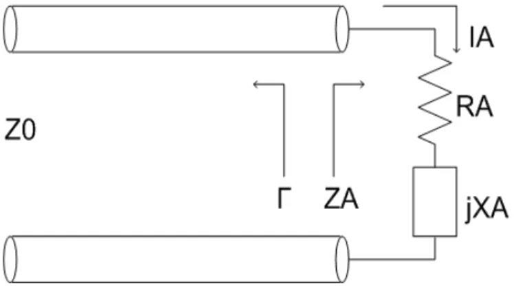
For single antenna case, the radiation efficiency is defined and computed by implementing the equivalent circuit shown in Figure 2.1[2].We can see that input impedance is composed of real part and imaginary parts:

A A A

Z =R +jX (2.1) The input resistance RArepresents dissipation, which occurs in two ways. Power that leaves

(18)

7

the antenna and never returns (i.e.,radiation) is a form of dissipation. There is also ohmic loss associated with heating on the antenna structure. The input reactance XA represents the power

stored in the near field of the antenna.

Figure 2.1 The equivalent circuit of single antenna in transmitting mode. The average power dissipated in an antenna is:

2

1 2

in A A

P  R I (2.2) where IA is the current at input terminals. Separating the dissipated power into radiative and

ohmic losses gives:

2 2 2 1 1 1 2 2 2 in ohmic A A r A ohm ic A P P P R I R I R I     (2.3) The radiation efficiency is defined as the ratio of total radiated power to the net power accept by the antenna, so r o h in o h m ic r o h m ic P P R e P P P R R      (2.4) The total radiation efficiency must take input mismatch effect into account. Therefore, the full expression of radiation efficiency on single antenna case is:

1 1

rad refl oh

e



e

(2.5) and

e

refl1



1  

2and 0

0 -A A Z Z Z Z    (2.6)

(19)

8 transmission line.

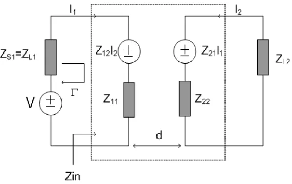
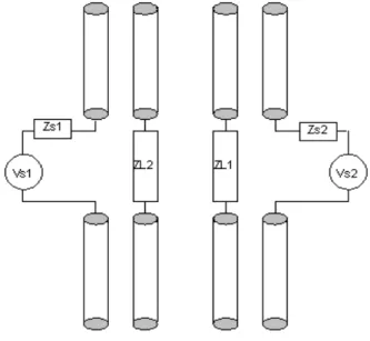
Figure 2.2 The equivalent circuit of an antenna pair in transmitting mode.

We further introduce the general definition of radiation efficiency in multiple antenna systems [5]. The radiation efficiency is defined mostly convenient in the transmit mode as the equivalent circuit shown in Figure 2.2. The voltage source V and source impedance ZS1 show

the excitation of the antenna port 1, and the load impedance ZL2 is the termination at the

second antenna port. Z12 is the mutual impedance which can describe the mutual coupling

effect between two antennas. For simplicity this equivalent circuit is constructed based on the antenna pair with identical structure, which means that Z11=Z22 and Z12=Z21.

The equivalent circuit in Figure 2.2 can be used to calculate the input impedance Zin,

which can further calculate the voltage reflection coefficient Γin. We can determine the input

impedance Zin as 1 2 12 11

I

Z

_in





(2.7) Equation (2.7) can be further expressed using the circuit loop theory which represents the relation between I1 and I2 as:

(20)

9 ₁ 2 22 12 2

I

Z

I

L







(2.8)

As a result, we can finally determine the input impedance Zin as:

2 22 2 12 11 L in

Z







(2.9)

The total power leaving antenna 1 is shown as PZin=(1/2)Real{Zin}|I1|2, and the power which

will be absorbed by ZL2 via mutual coupling effect and cause reduction of radiation power is

PZL2=(1/2)Real{ZL2}|I2|2. The difference between PZin and PZL2is called the radiation power Pr,

i.e., Pr= PZin- PZL2. Therefore, the radiation efficiency erad can be derived as

2 L Z refl rad

e



(2.10) where 2 ₁ 1 1 and in s refl in s Z Z e Z Z        (2.11) 2 1 2 2 2 2

}

{

Real

}

{

Real

1 I

Z

I

Z

e

in L ZL





(2.12)

The radiation efficiency is the composite power efficiency representation for it includes not only the reflection caused by input mismatch of the excitation port but also the power absorption resulting from the termination at the other unexcited antenna branch.

2.3 Antenna Spatial Correlation

Under multiple scattering environments, signal fading is the dominant impairment existing in the wireless communication. To overcome this problem multiple antennas are typically employed to provide diversity and the performance of the multiple antennas is determined by the spatial correlation between the antennas [6]. Antenna spatial correlation was first proposed by W. C. Jakes [7]. If a signal of interest arriving at an array can be

(21)

10

described by the summation of plane waves arriving from azimuth angle Φ relative to the normal between two sources a distance d apart, the spatial correlation can be determined as

)

(

))

sin(

2 exp(

)

(

_





 



_





d

j

d

p

d

(2.13) where λ is the wavelength and pΦ(Φ) is the azimuth angular probability distribution function.

The most special case is when pΦ(Φ)=1/2π which is called the Clarke’s model [8] and the

antenna spatial correlation has a closed form well-known as the Bessel function. Based on equation (2.13), several works on spatial correlation has relied on numerical integration or series expansion to evaluate the correlation coefficient between two sources based on different azimuth angular probability distribution functions [9-11]. The author in [12] especially discussed and derived a simple formula for spatial correlation and showed that it provided a good approximation for spatial correlation of small angular spread angular distributions.

The above definitions of antenna spatial correlation only take the signal phase and the angular PDF of the incoming waves in azimuth plane. Therefore, the antenna spatial correlation including full antenna patterns and mutual coupling effect was further proposed in the literatures. There were two main formulations proposed for the antenna spatial correlation including antenna patterns and mutual coupling effect. The first is direct Hermitian product of the far-field patterns between two antenna elements. The second is parameterized correlation formulation described by scattering matrix.

．Pattern Multiplication: This is the most direct but also the most complex definition. R. G. Vaughan and J. B. Andersen proposed in [6] that the spatial correlation is given by







        d F d F d F F 2 2 2 1 2 1 12 ) , ( ) , ( ) , ( ) , (          (2.14)

(22)

11

．Parameterized Formulation: The authors in [13] proposed exact representation of antenna envelope correlation in terms of scattering parameter description under the assumption of uniformly incoming waves. The approach has the advantage that it is not necessary to known the radiation pattern of the antenna system and that the explicit influence of mutual coupling and input match is revealed. The formulation is given by





2



21 2 22 2 12 2 11 2 22 21 12 11 2 12 1 1 S S S S S S S S env            (2.15)

Moreover, C. Waldschmidt and W. Wiesbeck further suggested a more general spatial correlation as [14] 2 2 2 1 12 12







R

(2.16) where 2 ₁ ₂ 12 0 0 1 2 2 2 2 2 0 0 ( , ) ( , ) ( , ) sin and ( , ) ( , ) ( , ) ( , ) ( , ) sin ( , ) ( , ) i i i XPR E E p R d d E E p XPR E p d d E p   _ _ _                                           _ _       _ _     _ _   

 

(2.17)

XPR is the cross polarization ratio, E is the far-field E antenna patterns, p(Φ,θ) means the AoA distribution, and the subscript Φ/θ denotes the field polarization for both AoA distribution and antenna patterns.

Compared with the pattern multiplication and the correlation represented in S-parameter manner, both of them do not take AoA distribution of arriving signals into account. Therefore, the spatial correlation in equation (2.17) is considered the most complete and general correlation formulation so far because it takes all the possible factors into consideration.

(23)

12

All the case studies we provide in the whole thesis are simulated using two or more half-wave dipole antennas. Therefore, the basic theory of half-wave dipole antenna is introduced in this section. The half-wave dipole antenna is the most general antenna structure, and the current distribution on the dipole usually assumes that the antenna is center-fed and the current vanishes at the end points. Moreover, to reduce the mathematical complexities, the diameter of the dipole is ideally much thinner than the wavelength of the operating frequency.

With the above assumptions, the current distribution is placed along the z-axis and for the half-sine wave current on the half-wave dipole. It is written as:

 

sin

, z

4

m

I z



I

_





_







z



_



_













(2.18)

where Im is the maximum current occurring at the center-fed point, andβis the phase constant

in the free space. After the cumbersome mathematical integration, the far-field Eθ pattern is

shown below:

cos

2

2 sin

j r m

I e

E

j

r

 



















































(2.19)

In the similar manner, the total HΦ component can be written as

cos

2

2 sin

j r m

E

I e

H

j

r

  



















































(2.20)

(24)

13

(a) (b)

Figure 2.3 (a) The λ/2 dipole and (b) the Eθ pattern in theta plane (Φ=0°).

The current distribution of the half-wavelength dipole and the theta-plane E-field pattern is plotted in Figure 2.3, and Zin=73+42j [2] .We need to notice that we assume the diameter of

the dipole is much thinner than the wavelength of the operating frequency, and there exists only Eθ and HΦ fields. However, in the chapter 4, EΦ and Hθ fields also exist in the simulation

results since the diameter of the dipole is not thin enough compared to the wavelength of the operating frequency.

(25)

14

Chapter 3 Composite Analysis of Radiation Efficiency

Antenna arrays play a crucial role in wireless communication over multipath fading channels. When using multiple antenna elements for implementation on small personal communications devices, the resulting closely spaced antenna elements exhibits well-known mutual coupling, which alters radiation pattern characteristics and is obviously impact the performance of multiple antenna systems. Radiation efficiency is considered an important factor to measure the performance of multiple antenna systems including mutual coupling. In this chapter, the analysis of radiation efficiency is in transmitting mode. The general definition of radiation efficiency for dual antenna systems has been introduced in Chapter 2 and we continue this concept for the further investigations on the composite analysis of reflection coefficient and radiation efficiency. In Section 3.1, the power representation using microwave network theory and TARC are first introduced as well as the concept of [16] . The composite analysis of how different kinds of termination network impact on the reflection coefficient and radiation efficiency are conducted in Section 3.2.

3.1 Introduction of The Eigenvalue based TARC and

Radiation Efficiency

3.1.1 Multi-port Antennas and Total Active Reflection

Coefficient

(26)

15

Assume that the scattering matrix of passive n-port antennas is S. The input excitation signals ai incident on each port i is denoted as the form of column vector a= [a1 , a2,…,an]T,

Similarly, the wave reflected from the antenna is denoted by the column vector b= [b1 ,

b2,…,bn]T [15][16] , the relation between a and b is



b

Sa

(3.1) The total powers incident on the n-port network is given by

2 2 1 N in i i

P

a



a



a a

H





(3.2) and the total power reflected from the n-port network is

2 2 1 N refl i i

P

b



b



b b

H



_

(3.3) The total input and reflected power can be represented as the summation of individual power incident on and reflected from the port i, respectively. The multiport antennas discount antenna ohmic loss for simplicity to analysis. First, we give an alternative expression to total reflected power and then we turn to calculate the radiated power. By substituting equation (3.1) into equation (3.3), the total reflected power can be written as:



 



refl

P



H H H H

Sa

= a S Sa

a Ra

(3.4)

,where R we call it reflection power matrix . This expression relates total power generated by excitations and the total reflected power. We now want to represent equation (3.4) in an alternative way for convenience to later analysis. Since the reflection power matrix is a Hermitian matrix, we can perform unitary similarity transformation [16] on R and U is unitary (i.e, UUH=I ) as below

(27)

16

H S

R = U D U with DS diag



_s₁,_s₂,K ,_sn



where

n n

R 



S

D (3.5) This transformation is also called eigenvalue decomposition (EVD). Substituting equation (3.5) into equation (3.4), an alternative representation of total reflected power is shown as













2 1

refl N i si i

P

q







H H s H H H s

a

U D U

a

U a

D

U a

(3.6) where

q = U a

H or

q

_i

= u a

iH (3.7)

The i th column vector of matrix U is denoted as Ui . Note that Ui is also an eigenvector of

reflection power matrix .qi can be viewed as a transformed input signal at port i. Using the

fact of UUH=I, the total input power can also be derived as



 



2 1

in N i i

P

q





H H H H

a a

U a

(3.8)

The power radiated by the antenna neglecting antenna ohmic loss is the difference between Pin

and Prefl, further substitution yields as below like [16]





2 2 2 1 1 1

1

rad in refl N N N i i si i si i i i

P

q



q



  



















(3.9)

The behavior of this microwave network is primarily defined by λsi. For a lossless network, Prad=0 so that λsi=1 for all i. For a lossy network like multiport antennas, Prad>0 so that 0≤ λsi

<1 for all i. As a result, EVD for reflection power matrix facilitates analysis and provides a useful interpretation of circuits’ fundamental behavior.

(28)

17

total active reflection coefficient (TARC) [17] is defined as the square root of the available power generated from all excitations minus radiated power, divided by the available power as

in rad in P P P TARC    (3.10)

For example, if an N-port antenna is excited at ith port and the other ports are connected to the matched load, the TARC can be calculated as

2 1

1 1,

.,

N i TARC ri ji j

p

s

i

N











_

 

_(3.11)

For multiport excitation, the TARC is therefore in the form of

2 1 2 1 N i i TARC _N i i

b

a

 







(3.12)

The TARC is a real number between zero to one. When the value of the TARC is equal to zero, all the delivered power is radiated and when it is equal to one, all the power either reflects back or goes to the other ports. This parameter is developed to describe the properties of multi-port antennas like frequency bandwidth and radiation performance, while all ports simultaneously excite signals with their own port impedances. In this manner, one is able to assess the true bandwidth of the antenna for a desired port excitation. This bandwidth information should give the multi-port antenna designer a much better understanding of the antenna bandwidth.

3.1.2 Eigenvalue Representation of TARC and Radiation

Efficiency

(29)

18

Section 2.2.Now the alternative definition of radiation efficiency is discussed in [16]. Before the derivation of radiation efficiency, we first give an alternative representation for TARC. Substituting equation (3.6) and equation (3.8) into equation (3.12), a new representation of TARC is defined as below

2 1 2 1 N i si i TARC _N i i

q



 







(3.13)

Since this expression is based on the eigenvalues of the reflection power matrix, we redefine it as eigenvalue based reflection coefficient (EVRC) for convenient to analysis and further derive an alternative representation of radiation efficiency as below which is similar with [16]and[20]









2 2 1 2 1

1

N i si i rad EVRE N i i

q

e

q



 





 





(3.14)

We rename this radiation efficiency as eigenvalue based radiation efficiency (EVRE) for simplicity of the following writing. It is wondered what is the difference between equation (3.14) and equation (2.10). Equation (2.10) is considered the composite power efficiency representation. It includes not only the reflection caused by input mismatch of the excitation port but also the power absorption resulting from the termination at the other unexcited antenna branch. Based on this definition, we may find equation (2.10) is actually a special case of equation (3.14). Taking a dual-antenna system for example, equation (2.10) will let one branch of the dual antenna system excite signals and the other terminated with impedance load. While in equation (3.14), two ports of the antenna system simultaneously excite signal with their own port impedances. That exactly means if we determine the radiation efficiency

(30)

19

using equation (3.14) but with one branch feeding signals of zero amplitude, the analysis result will be the same as that using equation (2.10).

One of the advantages of the EVRE is it takes into account the effect when ports of the multiple antennas system are fed with signals of different phases. EVRC (TARC) is originally developed for signals with various phase delays for multi-polarization operations, and this concept can be further extended to the multiple antennas system [18]. It is well known that mutual coupling causes some portion of signal power within each element to be radiated and absorbed by the other elements. The combination of each antenna port’s primary reflected signal with the coupled signals can be constructive or destructive depending on the phase of the component signals. EVRE of multiple antennas can therefore represent the effect of this constructive or destructive signal combination. Another way to show the effect of input excite signal phase difference on EVRE is based on the perspective of mathematical formulation as below: For dual antennas case and based on equation (3.13), the transformed input excitation signal is shown as

 

1 11 21 11 21 12 22 2 22 12

1

j j j

q

u

u e

u

e

q

u e

u

  



       







 











_

_



_

_{ }

_



_

_



























H

q

U a

g

(3.15)

, where θ is the phase difference of input excitation signals and the more explicit EVRC and EVRE are shown as

 









2 2 11 21 1 22 12 2 2 2 11 21 22 12 2 2 11 21 1 22 12 2 2 2 11 21 22 12

1

j j s s EVRC j j j j s s rad j j

u

u e

u

u e

u

u e

u

and e

u

u e

u

       









               



















(3.16)

As a result, it can be obviously viewed from equation (3.16) that EVRC and EVRE are indeed a function of input excitation signal phase difference.

(31)

20

The most important advantage of EVRC and EVRE are that they provide a simple way to estimate the minimum and maximum values of reflection coefficient and radiation efficiency quickly, no matter how many number of antennas will be gauged [16]. These advantages are revealed by further deriving equation (3.13) as an inequality and it is shown below

2 1 min max 2 1 N i si i s _N s i i

q













(3.17)

It is interesting that the minimum and maximum values of EVRC are just the square root of minimum and maximum eigenvalues of the reflection power matrix, respectively. The significances of the minimum and maximum values of EVRC are that they represent lowest reflection power and largest reflection power in the multiple antenna systems, respectively. Moreover, there exist no input excitation signal components to reach the EVRC lower than

min

s



or higher than



smax . Furthermore, based on equation (3.17) we can also derive an

inequality for EVRE and it is shown like [16] as below:

max min

1 



_s



e

_rad

 

1 

_s (3.18) Equation (3.18) means that the minimum or maximum EVRE occurs when maximum or minimum EVRC takes place at the same time. This phenomenon makes sense since the higher the reflection power occurs, the lower the power will radiate. Minimum and maximum values of EVRE are also considered two important quantities to judge the performance of multiple antenna systems.

What kinds of input excitation signal components will cause the maximum or minimum radiation efficiency is the another important issue. Another important advantage of EVRC and EVRE are that they both provide a convenient way to determine the input excitation signal components which may cause the best or worst case reflection coefficient and the

(32)

21

corresponding radiation efficiency, respectively. A mathematical proving is shown by further deriving equation (3.4) and using the result of equation (3.8) as follow: When the ith input excitation signal vector is the eigenvector of the reflection power matrix, the ith total reflection power can be determined as

  

   



2 2 1 1 N N i i i i i i i refl si si j si j j j

P



a



q

 



a

H

R a



a

H

a



_



_

(3.19)

,where ai is the ith input excitation signal vector and λsi is the corresponding eigenvelue. Moreover, we further derive the ith EVRC and EVRE as below [16]

2 1 2 1

and

1

N i si j j i i EVRC N si rad si i j j

q

e

q



 





 



(3.20)

By comparing the results between equation (3.19) and equation (3.20), we can observe that when the input excitation vector is the eigenvector of reflection power matrix, the minimum or maximum EVRC has the chance to be excited, and so does the corresponding EVRE. By utilizing unitary similarity transformation on reflection power matrix, we can easily find the corresponding input excitation signal components with the observation on the transformation matrix U when minimum or maximum EVRC takes place, and so does the corresponding EVRE. The applications and meanings of this powerful analysis strategy will be shown and discussed in the next section.

(33)

22

Figure 3.1 HFSS simulation setup of dual antennas configuration

Two parts of simulation results are provided in this section. First of all, we compare what is difference between conventional radiation efficiency using equation (2.10) and EVRE using equation (3.14), respectively. Secondly we offer a case study and show how the quantity of antennas affects EVRE. Moreover, we also discuss why EVRE provides powerful analysis for multiple antenna systems. We implement the case study with EM simulation software Ansoft® HFSS, while simulation programs are written in MATLAB® and run on PC with an Intel® Pentium IV 3-GHz CPU.

For convenience, the simulation environment is set with multiple dipole antennas. Figure (3.1) depicts the geometry for dual antennas. For the number of antennas is more than two, the setup of multiple antennas follows the same way as Figure (3.1), which is in symmetrical and parallel configuration. The radius of the dipole antenna is λ/100 and the dipole length is tuned at 0.44λ in order to make the dipole antenna resonant at the desired central frequency. In this work the central frequency is 2.45 GHz and the port impedance is set to be 50 Ohm.

(34)

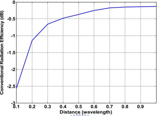
23 0.1 0.2 0.3 0.4 0.5 0.6 0.7 0.8 0.9 -3 -2.5 -2 -1.5 -1 -0.5 0 Distance (wavelength) C o n v e n ti o n a l R a d ia ti o n E ff ic ie n c y ( d B ) Figure 3.2 Conventional radiation efficiency analysis using equation (2.10).

0.1 0.2 0.3 0.4 0.5 0.6 0.7 0.8 0.9 1 -6 -5 -4 -3 -2 -1 0

Element Spacing (wavelength)

E V R E ( d B ) 0 10 20 30 40 50 60 70 80 90 100 110 120 130 140 150 160 170 180 180 degree 0 degree Phase Difference

Figure 3.3 EVRE analysis using equation (3.14)

Figure 3.2 and Figure 3.3 represent the conventional radiation efficiency analysis using equation (2.10) and EVRE analysis using equation (3.14), respectively. We assume port 1 is excited with 0.707 amplitude signal and port 2 is excited with 0.707*exp(jxπ/180°) where

(35)

24

x={0°,10°, 20°, …,180°}. One reason we let both the amplitudes of the input signals to be 0.707 is that we want to maintain the summations of all input excitations power unity and both ports have equal power. This set up contains a range of excitations with same amplitude but different phase offset distribution. By comparing these two figures, we observe that the phase difference between two antenna elements deeply affects the radiation performance and the newly-defined EVRE has the ability to show this effect. From Figure 3.3, we can observe that the performance of EVRE gets worse when the phase difference becomes large. The best radiation performance takes place when the two input signals are in phase, while the worst performance occurs when the two excitations are out of phase.

0.1 0.2 0.3 0.4 0.5 0.6 0.7 0.8 0.9 1 -20 -18 -16 -14 -12 -10 -8 -6 -4 -2 0

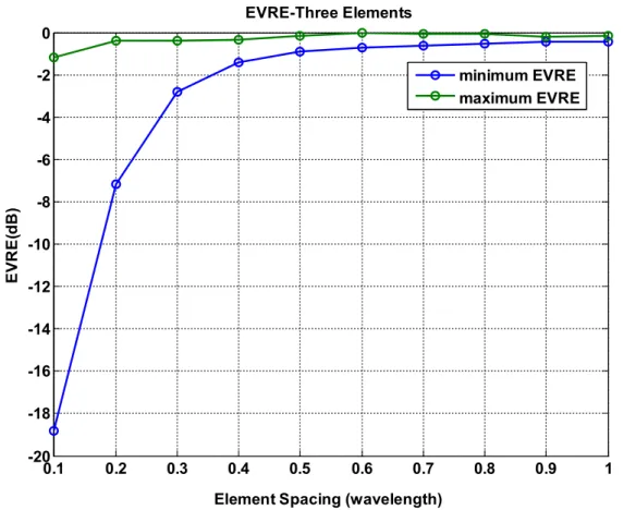
E V R E (d B ) EVRE-Three Elements minimum EVRE maximum EVRE

(36)

25 0.1 0.2 0.3 0.4 0.5 0.6 0.7 0.8 0.9 1 -35 -30 -25 -20 -15 -10 -5 0

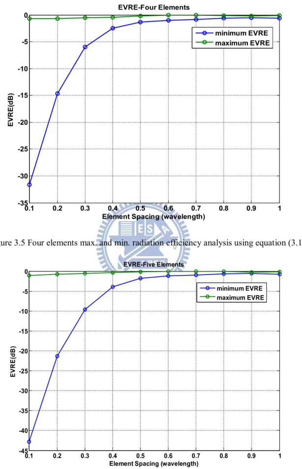
E V R E (d B ) EVRE-Four Elements minimum EVRE maximum EVRE

Figure 3.5 Four elements max. and min. radiation efficiency analysis using equation (3.16)

0.1 0.2 0.3 0.4 0.5 0.6 0.7 0.8 0.9 1 -45 -40 -35 -30 -25 -20 -15 -10 -5 0

E V R E (d B ) EVRE-Five Elements minimum EVRE maximum EVRE

(37)

26

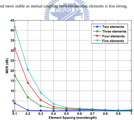
Finding the best or worst performance of EVRE for the number of multiple antennas more than two becomes cumbersome if we use the same way as dual antennas case presented before. However, it becomes easily and quickly to obtain the maximum and minimum values of EVRE by utilizing equation (3.16), which can be easily derived from equation (3.14) or equation (3.15). Figure 3.4 to Figure 3.6 represent the results when the number of antenna becomes three to five. We first define a parameter called Maximum Efficiency Ratio (MER), which means the ratio in dB between the maximum and the minimum EVRE to facilitate analysis. An observation from Figure 3.4 to Figure 3.6 is if the antenna elements are in close proximity, the radiation efficiency will have larger MER which means the performance may be very good or very bad at a given close antenna element spacing. The MER will become smaller as the antenna element spacing increase, which means the performance becomes better and more stable as mutual coupling between antenna elements is less strong.

0.1 0.2 0.3 0.4 0.5 0.6 0.7 0.8 0.9 1 0 5 10 15 20 25 30 35 40 45

M E R ( dB ) Two elements Three elements Four elements Five elements

(38)

27

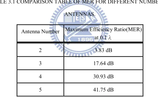
As the number of antenna elements increases, the maximum EVRE maintains almost the same while the minimum EVRE decreases a lot at fixed element spacing. The MER therefore becomes larger as shown in Figure 3.7 and a comparison table is shown as in TABLE 3.1.Take 0.1λ inter-element spacing as an example, the MER increases from 3.8 dB to 42 dB while the number of antenna increases from two to five which show the same tendency as the diagram depicted in [16]. The reason for this fact may due to higher mutual coupling and it results in more input mismatch effects at the central elements of these symmetrical multiple antenna sets when the number of antennas increase. As a result, there exists a set of input excitation signal components which cause the minimum EVRE worse.

TABLE 3.1 COMPARISON TABLE OF MER FOR DIFFERENT NUMBER OF ANTENNAS.

Finding the corresponding input excitation signal components when the best or the worst performance of multiple antenna systems (Maximum EVRE or Minimum EVRE) takes place by trying an error is nearly impossible when the number of antennas is more than two. By utilizing the eigenvalue decomposition shown in equation (3.17) to equation (3.19), these input excitation signal components are easily determined simply by solving the eigenvectors of reflection power matrix. The results are shown in Table 3.2 and Table 3.3 taking

Antenna Number Maximum Efficiency Ratio(MER) at 0.1λ

2 3.83 dB

3 17.64 dB

4 30.93 dB

(39)

28

0.1λinter-element spacing as an example. One thing to be mentioned is that the summation of the power from every port is equal to unity.

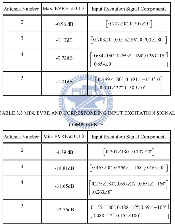
TABLE 3.2 MAX. EVRE AND CORRESPONDING INPUT EXCITATION SIGNAL COMPONENTS.

Antenna Number Max. EVRE at 0.1λ Input Excitation Signal Components

2 _{-0.96 dB} __{0.707 0 , 0.707 0}_ _ _   o o 3 _-1.17dB __{0.703 0 , 0.013 86 , 0.703 180}_ _ _ _  o o o 4 -0.72dB 0.654 180 , 0.269 164 ,0.269 16 , 0.654 0            o o o o 5 -1.01dB 0.589 180 , 0.391 153 , 0 , 0.391 27 , 0.589 0            o o o o

TABLE 3.3 MIN. EVRE AND CORRESPONDING INPUT EXCITATION SIGNAL COMPONENTS.

Antenna Number Min. EVRE at 0.1λ Input Excitation Signal Components

2 _{-4.79 dB} __{0.707 180 , 0.707 0}_ _ _   o o 3 _-18.81dB __{0.463 0 , 0.756}_ _{ }_{158 , 0.463 0}_ _  o o o 4 -31.65dB 0.275 180 , 0.657 17 , 0.651 164 , 0.263 0            o o o o 5 -42.76dB 0.155 180 , 0.488 12 , 0.69 165 , 0.488 12 , 0.155 180             o o o o o

(40)

29

An observation from Table 3.2 is that the power and phase of the input excitation signal at each port should be properly distributed and adjusted in order to reach the best performance. However, Table 3.3 gives us information that we should avoid exciting such input excitation signal components which will cause the worst performance. The eigenvalue representations of TARC and radiation efficiency in [16] provide us a quickly way to determine the best and worst radiation efficiencies and their corresponding input excitation signal components.Based on [16] we do further analysis on its characteristics in the following chapter.

3.2 Composite analysis of Termination Networks on TARC

and Radiation Efficiency

It has been shown that different kinds of termination networks may have great impact on conventional radiation efficiency [5]. In this section, the impact of termination networks including 50-Ohm, self-impedance and input impedance termination networks on EVRC and EVRE are investigated accordingly. A thoroughly comparisons about the performances of these three termination networks are also conducted in this section.

(41)

30

3.2.1 50-Ohm Termination Network

The simulation setup is shown as in Figure 3.8 and both the antennas are identical and have the same conditions as the previous section. It means that ZL1(=ZS1 when port 2 excitation)

and ZL2(=ZS2 when port 1 excitation).ZS1=ZS2=50 Ohm first comes as the first case study. It is

the most common topology for its wideband characteristic and easier implementation. Figure 3.9 and Figure 3.10 respectively show the maximum and minimum values of EVRC and EVRE using equation (3.15) and equation (3.16). Note that the reflection swing range here is defined as the difference between maximum and minimum EVRC, where the radiation swing range is defined as the difference between maximum and minimum EVRE.

0.1 0.2 0.3 0.4 0.5 0.6 0.7 0.8 0.9 1 0 0.1 0.2 0.3 0.4 0.5 0.6 0.7 0.8 0.9

E ig e n v a lu e b a s e d R e fl e c ti o n C o e ff ic ie n t Max-EVRC Min-EVRC

(42)

31 0.1 0.2 0.3 0.4 0.5 0.6 0.7 0.8 0.9 1 0.4 0.5 0.6 0.7 0.8 0.9 1

E ig e n v a lu e b a s e d R a d ia ti o n E ff ic ie n c y Max-EVRE Min-EVRE

Figure 3.10 Max. and min. EVRE of 50-Ohm termination network

3.2.2 Self-Impedance Termination Network

The termination network such as ZS1=ZS2=Z11* is known as the self-impedance source

matching (termination) network, which is also known as complex conjugate match and it facilitates maximum power transfer to the load when there is no mutual coupling. The goodness of the match depends on the behavior of the mutual impedance which is not taken into account. What can be mentioned in this simulation procedure is we do not need to re-simulate the dual antenna systems which use 50-Ohm port termination in the previous section to solve the new scattering matrix. However, by using the formulation as below

]

[

]

[

]

[

S

_new



ZZ

_port1



U

1

ZZ

_port1



U

(3.21) where Z is the impedance matrix, Zport is the diagonal matrix with diagonal terms(=ZS1 and

ZS2), and U is the unitary matrix, the new scattering matrix Snew can thus be computed and

(43)

32

the maximum and minimum value of EVRC and EVRE using equation (3.15) and equation (3.16). 0.1 0.2 0.3 0.4 0.5 0.6 0.7 0.8 0.9 1 0.1 0.2 0.3 0.4 0.5 0.6 0.7 0.8 0.9

Figure 3.11 Max. and min. EVRC of Z11* termination network

0.1 0.2 0.3 0.4 0.5 0.6 0.7 0.8 0.9 1 0.2 0.3 0.4 0.5 0.6 0.7 0.8 0.9 1

E ig e n v a lu e b a s e d R a d ia ti o n E ff ic ie n c y Max-EVRE Min-EVRE

(44)

33

3.2.3 Input-Impedance Termination Network

Input-impedance matching termination is considered more complete for it takes into account not only the reflection from the single antenna element but also the mutual coupling effect which results from the adjacent antenna element. It refers to maximum power transfer from the single excited source into the corresponding antenna port, which gives no consideration to power coupled into adjacent antenna. Because ZS1 is the function of ZL2

and vice versa, we may finally derive ZS1, based on equation (2.9) and ZS1=Zin*, as

























₁₁ 11 12 12 2 11 2 12 2 12 2 12 2 12 2 11 1

X

R

X

R

j

R

X

R

X

R

Z

_S (3.22)

where R11 and X11 are the real and imaginary part of self impedance, R12 and X12 are the real

and imaginary part of mutual impedance. Moreover, the new scattering matrix with Zin* port

termination can also be computed and used in calculation of EVRC and EVRE by equation (3.15) and equation (3.16). Figure 3.13 and Figure 3.14 respectively show the maximum and minimum value of EVRC and EVRE using equation (3.15) and equation (3.16).

0.1 0.2 0.3 0.4 0.5 0.6 0.7 0.8 0.9 1 0.1 0.2 0.3 0.4 0.5 0.6 0.7 0.8

數種新型多天線系統分析方法

國

立

交

通

大

學

電信工程學系

碩

士

論

文