Cross-Reference Weighted Least Square Estimates
for Positron Emission Tomography
Henry Horng-Shing Lu,* Chung-Ming Chen,
Member, IEEE, and I-Hsin Yang
Abstract— An efficient new method, termed as the cross-reference weighted least square estimate (WLSE) [CRWLSE], is proposed to integrate the incomplete local smoothness information to improve the reconstruction of positron emission tomography (PET) images in the presence of accidental coincidence events and attenuation. The algebraic reconstruction technique (ART) is applied to this new estimate and the convergence is proved. This numerical technique is based on row operations. The computational complexity is only linear in the sizes of pixels and detector tubes. Hence, it is efficient in storage and computation for a large and sparse system. Moreover, the easy incorporation of range limits and spatially variant penalty will not deprive the efficiency. All this makes the new method practically applicable. An automatically data-driven selection method for this new estimate based on the generalized cross validation is also studied. The Monte Carlo studies demonstrate the advantages of this new method.
Index Terms—Algebraic reconstruction technique, generalized cross-validation, regularization, weighted least square estimate.
I. INTRODUCTION
M
ODERN commercial positron emission tomography (PET) systems are able to take into account the acci-dental coincidence (AC) events and attenuation to improve the PET image reconstruction [1]. The AC events introduce nui-sance parameters and make it difficult for the reconstruction. Fessler [2] proposed a penalized weighted least square method with a nonnegative successive over-relaxation algorithm to handle these problems. The penalized weighted least square reconstruction can be accelerated if simple unbiased estimates and row operation iterative methods, such as the algebraic reconstruction technique (ART) [3]–[5], are considered. The computational complexity and the storage cost of ART are less. The constraints in the reconstruction of images, such as nonnegativeness, can be incorporated in the ART without any difficulty at the same time. These advantages make the ART the right technique to be investigated.Since the random observations are indirectly related to the target image, the problem of reconstruction is ill posed. Due to this ill-posed nature of inverse problems, the estimates of PET images, such as the maximum-likelihood estimate,
Manuscript received December 19, 1996; revised November 10, 1997. This work was supported by the National Science Council of Taiwan. The Associate Editor responsible for coordinating the review of this paper and recommending its publication was Y. Censor. Asterisk indicates corresponding author.
*H. H.-S. Lu is with the Institute of Statistics, College of Science, National Chiao Tung University, Hsinchu, Taiwan (e-mail: [email protected]).
C.-M. Chen is with the Center for Biomedical Engineering, College of Medicine, National Taiwan University, Taipei, Taiwan.
I.-H. Yang was a graduate student in the Institute of Statistics, National Chiao Tung University, Hsinchu, Taiwan.
Publisher Item Identifier S 0278-0062(98)03122-X.
WLSE, and other estimates, without regularization will lead to undesirable spiky images with edge and noise artifacts [6]. While a penalty term is necessary to regularize the estimation, the choice of penalty term is important to obtain a sensible solution. The choice of which shall not depend solely on the mathematical convenience, but will depend on the bona fide correlated information. Ouyang et al. [7] have suggested a sophisticated path to incorporate the correlated boundary information in a Bayesian setup, though the computation is quite demanding. Inspired by their work, an attempt is made to incorporate the correlated local but incomplete structure information in weighted least square method through a compu-tationally efficient route. First, a penalty term is considered that describes the spatially variant smoothness in the penalty term. Then, the ART is applied to this specific type of penalized weighted least square estimate (WLSE). The resulting method, which is termed a cross-reference WLSE (CRWLSE), turns out to be quite alluring, as demonstrated in this article.
A physical and mathematical model of PET with AC events and attenuation is introduced in Section II. The estimation and computational methods of WLSE are discussed in Section II. A possible regularized (or penalized) WLSE with global penalty term and the related ART is investigated in Section III. An efficient and new approach, the CRWLSE, to incorporate the correlated but incomplete information about local smooth-ness is proposed in Section IV. The computational aspects and the selection of penalty parameters are discussed as well in Section IV. Finally, the conclusion and discussion of the related issues about the CRWLSE is given in Section V. All the proofs of theorems are in the Appendix.
II. A MODEL AND THE WLSE A. Model Setups
An ideal model of PET without AC events and attenuation was introduced in [8] and [9]. Initially, positrons are emitted
at the box , , and these positrons hit
nearby electrons to annihilate themselves. Thereafter, a pair of photons are generated, which travel in the opposite direction of a line. These photon pairs are detected by a pair of scintillation detectors outside a human body within a very short time difference and, thus, form a coincidence event. However, in practice, before these pairs of photons arrive the detectors, their energy will be attenuated by the Compton scattering while passing through the body tissues. Therefore, a part of these photon pairs will not have energy greater than the threshold level of detectors. Thus, they remain undetected.
Hence, only the survived portion of the attenuated photon pairs are recorded, which can be described by a survival probability [10]. It is observed that besides these losses due to attenuation, the detectors may receive other photon pairs that are not generated by the annihilations which occur at the target image in a specific slice of a human body. That is, there are AC events. The observation made by a detector pair is the sum of photon pairs which occur at the target image and the AC events. Therefore, to recover a true image, one can subtract the number of photon pairs due to the presence of AC events [2], [10].
Suppose the target image is partitioned into boxes (or pixels) and there are detector tubes. For each pixel
and each tube , the following
notations are adopted.
Emission intensity of the target at pixel . Probability of an emission from box being de-tected along the detector tube .
Survival probability that an emission photon pair from box traveling in tube will have energy greater than the threshold level of detectors after attenuation.
With attenuation, the transition probability becomes (1) In order to correct the AC events, the recent generation of commercial PET systems use prompt (or real-time) window coincidences to subtract the random coincidences of delay windows [1], [2]. The following notations are used.
Number of coincident photon pairs collected in the prompt windows at detector tube .
Number of coincident photon pairs collected in the delay windows at detector tube .
Furthermore, and are assumed to be statistically independent and Poisson distributed with different means
Poisson (2)
Poisson (3)
where “ ” means that the random variable “is distributed as,” is the mean intensity of and
(4)
One can define the precorrecting value in detector tube , by subtracting from
(5) However, can be negatively valued. Also, the mean and variance of are different when . Therefore, is not Poisson distributed. When , with probability one. Otherwise, by approximating the moment generating function in the neighborhood of zero, is approximately distributed as a normal distribution
with mean and variance . This will be
stated in the next Proposition.
Proposition 1: If or , then
where “ ” means that the random variable “is approximately distributed as.”
Therefore, the maximum-likelihood estimate of the approx-imate model is the WLSE. They are studied in the next subsection.
B. Estimation and Computational Methods
The following notations are introduced to simplify the expressions. Let (6) (7) diag (8) (9)
By the assumption or , for all
, is nonsingular and does exist. The WLSE needs to minimize . It is noticed that
(10) where
(11) Thus, one can return to the least square form after suitable transformation in (11). But, the variances, , is unknown. The sum value in detector tube is defined to be
by adding to
(12) Then, is an unbiased estimator of the unknown variances
. The variance and mean square error of are equal to . This is a direct and a fast way to estimate the variance of . If the observed value of is small, then the smoothed estimate, such as that in [2, Appendix], can be applied. This involves more computation. The mean square error can be reduced if the tradeoff between bias and variance is properly tuned.
Therefore, when , the th element of , can be estimated by and the th row of can be estimated by
Next, the case that is considered. Obviously,
. If , then
with probability one. Suppose or , then the following proposition can be proved.
Proposition 2: It is true that or
(13) Thus, the most likely case for is that
. That is, the WLSE is when .
Equivalently, can be replaced by zero and the th row
of can be replaced by when
. To sum up, the estimates for the th element of , , and the th row of , , are
if
if ; (14)
if ,
if .
(15) The resulting solution of least square form, , will be equivalent to the WLSE.
In addition, the reconstruction image intensity is needed to be nonnegative or within a range limit. This can be achieved by solving first the unconstrained problems and then projecting the solution to the constraint set (e.g., see the trick of constraining for ART [3, p. 194]). For notational convenience, , , , and are used to denote either their true values or estimates hereafter. The WLSE becomes
(16) The computational methods of WLSE can be achieved by applying the finite series expansion reconstruction methods [5], like the algebraic reconstruction technique (ART) [3], [4]. The idea of ART is to solve the system of equations successively, but not simultaneously. Thus, it is an iterative method based on row operations, which makes it efficient in computation and storage. The constraints of range limits, such as nonnegativeness, can be easily implemented in every iteration as well.
One way to use the ART is to solve the consistent system of normal equation
(17) together with the trick of constraining [3]. However, the total storage space for the symmetric square matrix is
large. For instance, it is 32
megabytes in floating format when . This will not occur if the ART without relaxation parameters is used to solve (18) directly since the large sparse matrix can be stored effi-ciently. Although the above system of equations (18) may be inconsistent, the ART without relaxation parameters can still generate a subsequence converging to the minimum norm least square solution when the initial solution is selected in the range space of (e.g., see [11, Corollary 9]). However, this kind of inconsistency problem will not occur when the ART is applied to the regularized WLSE (RWLSE) or CRWLSE in
the forthcoming sections since consistent systems of equations involving , but not , can be set up. The details of ART algorithm are demonstrated in Algorithm 1 of Section IV.
III. A RWLSEWITH A GLOBAL PENALTY
Due to the ill posedness, the reconstruction procedure needs to be regularized. One way to regularized the WLSE is to combine the (weighted) least square term and a penalty term into an object functional. That is, it is aimed to minimize
(19) where is a positive constant. The penalty parameter balances the tradeoff between the (weighted) least square term and penalty term. If , then it is reduced to the (weighted) least square term. If , then the penalty term dominates. The penalty term can be a norm or seminorm. For instance, the 2-norm, , can be considered. In the Bayesian framework, the penalty term is related to the prior.
For the minimum value of object functional
(20) there exists a unique solution for any . The resulting estimate is termed as the RWLSE
(21) The RWLSE without nonnegative constraints is
(22) This is also known as a ridge estimate in the setup of ridge regression [12]. More theoretical properties can be found in the setup of inverse problems [13] or statistical inverse problems [14].
From the aspects of computation, one does not want to solve the related normal equation derived from the object functional because the ingredient matrix takes too much storage space or computational time. With the introduction of a dummy variable , Herman et al. [4] suggested that instead a related consistent system of equations can be solved. Hence, the ART with or without relaxation parameters can be applied. In order to understand the mechanism behind their approaches, the result of the ART without relaxation parameters is explained, which is just the Kaczmarz’s iterative method in solving a system of linear equations. This iterative method performs the consecutive orthogonal projections onto the hyperplanes defined by the th equation, , where is the th row of . The following lemma explores the convergence and the properties of the convergent solution.
Lemma 1: The following three statements hold.
1) Let be the set of least square solutions of . The ART algorithm without relaxation parameters will generate a subsequence converging to
, where is an arbitrary initial vector, is the unique Moore–Penrose generalized (or pseudo) inverse of and is the orthogonal projection to the null space (i.e., kernel) of .
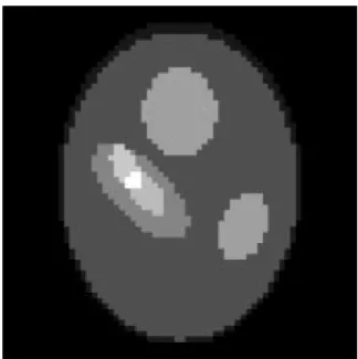
Fig. 1. A test phantom.
3) If is chosen to in the range space of , one has an additional property that , for all . The property 3) of the above Lemma is a generalization of the property of the pseudo inverse to that of the convergent point of the ART. The property 2) of the above Lemma is very useful since it holds for any possible . That is, will decide the destination of the convergent subsequence generated by ART algorithm without relaxation parameters for both consistent and inconsistent systems. If the initial vector is properly selected, then a lot of related problems can be solved. Given below is a typical one.
Theorem 1: If is the minimum norm solution of the consistent system of equations
(23) generated by the ART algorithm without relaxation parameters for an initial vector , where is a by identity matrix
and is a by one column vector, then minimizes in (20).
In order to see the results of this RWLSE, the following Monte Carlo simulation are performed. Suppose there are 30%
AC events, that is, and for
all . Let us assume the true phantom is as given in Fig. 1. The number of detectors is set to 64 and the number of pixels is . The number of detector tubes is smaller than and only about half of those detectors tubes can receive photon pairs generated from the target object [8]. The total detected coincidence events in prompt windows and delay windows are at the level of 90 000 and 20 000, respectively. This RWLSE with global penalty (21) will reconstruct an image as shown in Fig. 2.
The penalty parameter is chosen to minimize the 2-norm error between RWLSE and the true phantom. The reconstruction results in the oversmoothness due to which a lot of local structures get lost. This can be attributed to the global penalty used in this RWLSE. Ouyang et al.
Fig. 2. The RWLSE-ART reconstruction using a global penalty with a penalty parameter of 0.001 and four iterations.
[7] have tried to incorporate the local smoothness information to reconstruct better PET images. They had put together the prior boundary information with Gibbs’ sampling technique in the Bayesian framework. The computation turns out to be quite complicated and expensive. Therefore, a more efficient method to combine the local smoothness information for better PET reconstruction in the presence of AC events and attenuation is proposed in Section IV.
IV. CRWLSE A. The Reconstruction Method
Suppose that the boundary information is available as shown in Fig. 3. This information is incomplete because it does not include all the boundaries in the true phantom. By using the boundary location, we can get a mean estimate, , by taking the average intensities of within the informed boundaries. The resulting is shown in Fig. 4.
Since the boundary information may be incomplete or incorrect, can, thus, be served best as a reference point. The finer adjustment needs to be done by cross referring the weighted least squared part and the discrepancy to .
The above idea can be formulated through an optimization problem. Namely, the object functional now becomes
(24) where is a positive constant. This is equivalent to shift the origin to and find the least square solution that lies closest to the new origin. In the Bayesian framework, this can be regarded as the informative (or expertise) prior. In the setup of ridge regression, this represents the change of the origin to the mean value. All these different perspectives come to the same optimization problem. The unique existence and other theoretic properties may be derived as in the RWLSE after the
Fig. 3. The incomplete boundary information.
Fig. 4. The mean estimate based on the boundary information and WLSE-ART.
origin is shifted to . This solution is termed as a CRWLSE (25) Based on the results of Section III regarding the RWLSE, the ART can be used to solve this optimization problem if the initial value is properly selected. This can be demonstrated in the next theorem.
Theorem 2: If , then the iterative solutions of the consistent system of equations and
generated by the ART without relaxation parameters will converge to a solution that minimizes in (24).
Herman et al. [15] had generalized the ART algorithm
to include relaxation parameters for ,
for consistent systems. If , then this is equivalent
to the Kaczmarz’s method. If [or ],
then it is an under- (or over-) relaxation parameter. The results of convergence can be assured if the system of linear
equations is consistent and
[15]. The convergence of ART with strong underrelaxation parameters for inconsistent system of linear equations is shown in [16]. The relaxation parameters can be used to accelerate the convergence of ART.
Upon these results, the computation algorithm for the CR-WLSE along with relaxation parameters and the constraining trick can be generated. Suppose the constraints are
, that is, all lie between a lower and upper bound. For example, if the constraints are nonnegativeness, then . The trick of constraining is to let be in every iteration. The details of the computation algorithm are stated as follows.
Algorithm 1:
1) Choose the initial vector .
Let and . 2) . 3) For ; ; ; ; ; for ; ; ; end b; end j. 4) .
5) If , for a positive tolerance limit, , and a norm , say the 2-norm, then the iteration is stopped. Or else, go back to step 2.
The iteration procedure with or does not change the pattern of convergence of a consistent system of equations considered here because that the orthogonal projec-tions commute and all possible projecprojec-tions are performed after one iteration. It is noted that the computational complexity is only and the memory requirement is very small. The resulting CRWLSE is shown in Fig. 5.
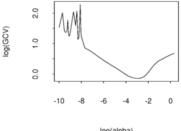
The penalty parameter is chosen according to the minimum of the generalized cross-validation (GCV) curve, as shown in Fig. 8, which is discussed in the next subsection. The comparative studies and the selection of penalty parameters are also addressed in the next subsection.
B. Selection of the Penalty Parameters
It is important to select the penalty parameter to balance the tradeoff between the least square term and smoothness term. Suppose the iteration number is fixed to be four, the 2-norm errors between the CRWLSE and the true phantom are plotted against the penalty parameter as shown in Fig. 6.
Fig. 5. The CRWLSE-ART reconstruction with a penalty parameter of 0.001 and four iterations.
Fig. 6. The 2-norm errors of the CRWLSE, the RWLSE, the WLSE, and the mean estimate with respect to penalty parameters for the entire image. The base of logarithm function is ten.
One can see that as , then the 2-norm errors of CRWLSE with respect to the true phantom approach to the 2-norm error of WLSE with respect to the true phantom. On the other hand, the 2-norm errors of CRWLSE approach to that of the mean estimate as . Between zero and , there exist proper parameters that minimize the 2-norm errors. Therefore, a dynamic graph technique, like a scroll box or a slider, that provides an interactive way for the user to select a proper parameter can improve the reconstruction image. Furthermore, the CRWLSE has smaller 2-norm errors than those of the WLSE and the RWLSE with the global penalty as shown in Fig. 6 for all penalty parameters. The CRWLSE can beat the mean estimate with a suitable choice of the penalty parameter.
One may ask the performance of CRWLSE for some par-ticular region of interest. For instance, the region of interest may be the region in the lower left part of Fig. 3 that does not have complete boundary information when it is compared with Fig. 1. This is a case when the anatomic boundary in prior
Fig. 7. The 2-norm errors of the CRWLSE, the RWLSE, the WLSE, and the mean estimate with respect to penalty parameters for a particular lower left region of interest. The base of logarithm function is ten.
information is not the same as the functional boundary in the true target. At first glance, it seems that the small lesions in that particular region are more evident of RWLSE as shown in Fig. 2 than those of CRWLSE as shown in Fig. 5. But, after careful examination, one finds that the locations of the small lesions of RWLSE as shown in Fig. 2 incorrect when they are compared with the true phantom in Fig. 1. If the 2-norm errors for various estimates of that particular region of interest are plotted, one can see that CRWLSE still outperforms the RWLSE and WLSE as shown in Fig. 7. With a suitable choice of the penalty parameter, the CRWLSE can beat the mean estimate.
Does there exist an automatically data-driven method to select a suitable penalty parameter? The answer is yes. For the ridge regression setup with zero as the origin, Golub et al. [12] generalized the ordinary cross-validation to the GCV to select the ridge parameter. The ordinary cross-validation is to delete one observation at one time and use the regression fit of the remaining observations to predict the deleted observation. Then, the sum of squares of predicted residuals, PRESS, can be calculated. But the PRESS is not rotational invariant. In order to make it rotational invariant, they consider the PRESS on a transformed model. The resulting form is called GCV.
Hence, it is possible to find the corresponding GCV for the CRWLSE. Through the shift of origin, the equivalent form of object functional can be derived as follows:
(26) where
(27) (28) Therefore, after the transformation in (27) and (28), the object functional become the standard form in ridge regression. Thus, the GCV can be applied to the CRWLSE. The choice
Fig. 8. The GCV curve with respect to penalty parameters.
of is the minimum of given by
(29)
where , and
, are the eigenvectors and eigenvalues of . The GCV curve is plotted in Fig. 8.
The eigenvalue or singular value decomposition (EVD or SVD) is essential to find out . For small to medium size matrices, the EVD for a symmetric matrix and SVD for any matrix can be found via the existing library functions, such as the imsl f eig sym and imsl f lin svd gen functions in the IMSL C/MATH library. For large size matrices, they can be explored through the power method together with the deflation [17]. In order to check the numerical correction, the errors of with 1-norm are inspected for all eigenvectors and eigenvalues . It is found that the errors in the large eigenvalues are large for the IMSL function and those in the small eigenvalues are large for the power method. This means that the leading portion of eigenvalues, but not the ending portion of eigenvalues, can be well located by the power method. The IMSL function is on the contrary.
One can observe that the minimum value of GCV curve as shown in Fig. 8 is slightly smaller than that of 2-norm errors shown in Fig. 6. Using this minimum value of GCV curve, the CRWLSE can be reconstructed as shown in Fig. 5. Thus, the GCV selection rule can provide a data-driven approach to suggest a penalty parameter. If an iterative selection rule using dynamic graphics is built in the reconstruction system, then the reconstruction image can be even improved upon using the initial penalty parameter suggested by the GCV selection rule. For the same true phantom as shown in Fig. 1, the even more incomplete and incorrect boundary information is also considered, which is at an incorrect alignment position with respect to the boundaries of the true phantom. The results of the experiments, which are not shown here to save space, reveal that the CRWLSE is quite robust to the selection of boundaries and mean estimates. The penalty parameters can act
as the fine tuners so that the CRWLSE can reconstruct a better image using incomplete and incorrect boundary information.
V. CONCLUSION AND DISCUSSION
Due to the presence of AC events and attenuation in the PET systems, the corrected observations no longer follow a Poisson distribution. A normal approximation is considered and the WLSE is investigated. Through cross-referring the boundary information, the reconstruction can be improved. Even with an incomplete and incorrect boundary information, it is observed that the CRWLSE can still outperform the WLSE and the RWLSE with global penalty. The improvements are observed both for the whole image and for the particular region of interest which does not have a correct boundary information. This is very useful because the anatomic and functional boundaries are usually different. Meanwhile, the penalty parameter in CRWLSE can be selected by users or through the automatically data-driven method, such as the GCV method.
The ART technique is considered here. The computational complexity of ART is . This complexity is the same as that of the expectation-maximization (EM) algorithm. It is smaller than , the complexity of the projected successive overrelaxation (SOR) method (i.e., the ICM method in the Bayesian setups, see Fessler [2]). The EM algorithm is a competing one to the ART and the ART works faster in unit computational cost. The one-step-late (OSL) approximation of the EM algorithm [18] for the CRWLSE was tried. The result-ing reconstructions were not good. Further examination of the EM algorithm for the purpose of cross-reference reconstruction is necessary. Hence, from the prospects of computational complexity, memory requirement and unit computational time per iteration, the ART is good for the reconstruction of CRWLSE. In addition, the constraints can be integrated with very small increase in the computational cost. The relaxation parameter can be utilized to accelerate the convergence of ART. This technique can also be combined with other tricks and can be generalized to handle the system of inequalities as summarized nicely in [3]. All these advantages make the ART the right technique for our purpose.
One can also use the EVD of to obtain the SVD of . Thus, the truncated singular value reconstruction for solving can be considered, which is equivalent to solving the normal equation with truncated SVD. The reconstruction results are blurry and spiky. This again shows the importance of regularization using boundary information of CRWLSE in the PET reconstruction. Finally, the empirical studies of CRWLSE are of great interest in our future research projects.
APPENDIX
Proposition 1 Proof: The moment generating function of can be derived as follows:
The moment-generating function can be approximated in the neighborhood of zero by
Proposition 2 Proof: Suppose and ,
then
because . Similarly, the other
two cases can be proved when and or
and .
Lemma 1 Proof:
1) It is shown in [11, Corollary 9].
2) It is noted that belongs the orthogonal complement of the null space of , that is, the range space of . Since both and belong to ,
, where is the orthogonal projection to the range space of . Hence, the difference, is in the null space of . So
3) If , an additional property is shown
Theorem 1 Proof: If one puts for any , then this will always be a solution of because
Hence, this is a consistent system and the solution set is the set of that satisfies . If the ART without relaxation parameters is used with initial vector , then the iterated sequence will converge to a solution that minimizes
via the Lemma 1.
Theorem 2 Proof: This proof is similar to that of Theo-rem 1. Since , the iteration will convergent to a solution that minimizes
ACKNOWLEDGMENT
The authors would like to thank I.-S. Chang, C. A. Hsiung, B. M. W. Tsui, and W. H. Wong for their discussions. They also thank the associate editor and referees for their valuable comments and suggestions.
REFERENCES
[1] T. J. Spinks, T. Jones, M. C. Gilardi, and J. D. Heather, “Physical performance of the latest generation of commercial positron scanner,”
IEEE Trans. Nucl. Sci., vol. 35, no. 1, pp. 721–725, 1988.
[2] J. A. Fessler, “Penalized weighted least-squares image reconstruction for positron emission tomography,” IEEE Trans. Med. Imag., vol. MI-13, pp. 290–300, April 1994.
[3] G. T. Herman, Image Reconstruction From Projections: The
Fundamen-tals of Computerized Tomography. New York: Academic, 1980. [4] G. T. Herman, A. Lent, and H. Hurwitz, “A storage-efficient algorithm
for finding the regularized solution of a large inconsistent system of equations,” J. Inst. Math. Applicat., vol. 25, pp. 361–366, 1980. [5] Y. Censor, “Finite series-expansion reconstruction methods,” Proc.
IEEE, vol. 71, no. 3, pp. 409–419, 1983.
[6] D. L. Snyder and M. I. Miller, Random Point Processes in Time and
Space, 2nd ed. New York: Springer-Verlag, 1991.
[7] X. Ouyang, W. H. Wong, V. E. Johnson, X. Hu, and C. T. Chen, “In-corporation of correlated structural images in pet image reconstruction,”
IEEE Trans. Med. Imag., vol. 13, pp. 627–640, Aug. 1994.
[8] L. A. Shepp and Y. Vardi, “Maximum likelihood reconstruction for emission tomography,” IEEE Trans. Med. Imaging, vol. MI-1, pp. 113–122, Oct. 1982.
[9] Y. Vardi, L. A. Shepp, and L. Kaufman, “A statistical model for positron emission tomography,” J. Amer. Stat. Assoc., vol. 80, no. 389, pp. 8–20, 1985.
[10] D. G. Politte and D. L. Snyder, “Corrections for accidental coinci-dences and attenuation in maximum-likelihood image reconstruction for positron-emission tomography,” IEEE Trans. Med. Imag., vol. 10, pp. 82–89, Feb. 1991.
[11] K. Tanabe, “Projection method for solving a singular system of linear equations and its applications,” Numer. Math., vol. 17, pp. 203–214, 1971.
[12] G. H. Golub, M. Heath, and G. Wahba, “Generalized cross-validation as a method for choosing a good ridge parameter,” Technometrics, vol. 21, no. 2, pp. 215–223, 1979.
[13] C. W. Groetsch, Inverse Problems in the Mathematical Sciences. Braunschweig, Germany: Vieweg, 1993.
[14] H. H.-S. Lu and M. T. Wells, “Adaptive constrained method of regular-ization estimators for latent density estimation,” National Chiao Tung University, Tech. Rep., 1994.
[15] G. T. Herman, A. Lent, and P. H. Lutz, “Relaxation methods for image reconstruction,” Commun. ACM, vol. 21, no. 2, pp. 152–158, 1978. [16] Y. Censor, P. P. B. Eggermont, and D. Gordon, “Strong underrelaxation
in Kaczmarz’s method for inconsistent systems,” Numer. Math., vol. 41, pp. 83–92, 1983.
[17] B. N. Parlett, The Symmetric Eigenvalue Problem. Englewood Cliffs, NJ: Prentice-Hall, 1980.
[18] P. J. Green, “On use of the EM algorithm for penalized likelihood estimation,” J. Roy. Statist. Soc., vol. B-52, no. 3, pp. 453–467, 1990.