MINLAB: Minimum Noise Structure for
Ladder-Based Biorthogonal Filter Banks
See-May Phoong, Member, IEEE, and Yuan-Pei Lin, Member, IEEE
Abstract—In this paper, we introduce a minimum noise structure for ladder-based biorthogonal (MINLAB) filter bank. The min-imum noise structure ensures that the quantization error has a unity noise gain, even though the filter bank is biorthogonal. The coder has a very low design and implementation cost. Perfect re-construction property is structurally preserved. Optimal bit alloca-tion and coding gain formulas are derived. We show that the coding gain of the optimal MINLAB coder is always greater than or equal to unity. For both AR(1) process and MA(1) process, the MINLAB coder with two taps has a higher coding gain than the optimal or-thonormal coder with an infinite number of taps. In addition to its superior decorrelation ability, it has many other desired features that make it a potentially valuable and attractive alternative to the orthonormal coder, especially for the high-fidelity compression.
Index Terms—Biorthogonal, compression, filter bank, minimum noise, subband coding, wavelet coding.
I. INTRODUCTION
R
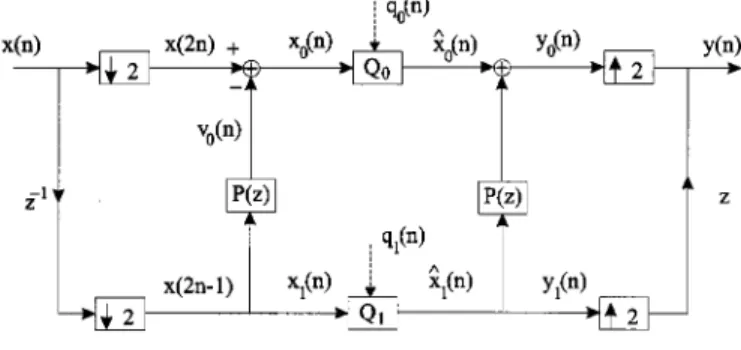
ECENTLY, there has been considerably interest in ap-plying the ladder structure to data compression [1]–[17]. Fig. 1 shows a simple two-channel filter bank (FB) that uses only one ladder. Such a structure is also known as the lifting scheme in wavelet coding [6], [7], [16]. In the absence of the quantizers, such a biorthogonal system always has the perfect reconstruction (PR) [18], that is, for all possible , regardless of the choice of . In other words, the FB is structurally PR. The analysis filters and synthesis filtersare, respectively
(1) The implementation and design of the biorthogonal system in-volves only , and hence, the design and computational cost is very low. Even though the filters in (1) are simple, their coding performance is comparable with that of orthonormal coders. Note that such a FB can never be orthonormal unless is zero.
The ladder structure is first applied to progressive coding in [1]. It is shown in [2] how roundoff noise of the ladder structure at the encoder is cancelled by that at the decoder. A special Manuscript received September 16, 1998; revised May 30, 1999. This work was supported by the NSC under Grants 88-2213-E-002-080 and NSC 88-2218-E-009-016, Taiwan, R.O.C. The associate editor coordinating the review of this paper and approving it for publication was Dr. Xiang-Gen Xia.
S.-M. Phoong is with the Department of Electrical Engineering, Institute of Communication Engineering, National Taiwan University, Taipei, Taiwan, R.O.C. (e-mail: [email protected]).
Y.-P. Lin is with the Department of Electrical and Control Engineering, Na-tional Chiao Tung University, Hsinchu, Taiwan, R.O.C.
Publisher Item Identifier S 1053-587X(00)01009-6.
useful class of ladder structure is used as a framework for the construction of causal stable PR IIR FB [3], [4]. The same framework can be generalized to the quincunx (two-dimen-sional) 2-D FB by using a simple one-dimensional (1-D)-to-2-D mapping [4], [5]. In [6] and [7], the ladder structure or so-called lifting scheme is employed to construct biorthogonal wavelets and wavelets defined on irregular sampling grid. It was shown in [8] that both orthogonal and biothogonal FB can be factorized into lifting steps. The nonlinear operator is used in the ladder structure to generate nonlinear FB with PR property [9], [10]. A low-cost and useful nonlinear operation is introduced in [10], and it is shown that the nonlinear FB coders have the ability to preserve edges and remove the blocking and ringing effects of compressed images. The ladder structure has also been applied to lossless and lossy coding of images, and satisfactory coding results can be obtained. In [11] and [12], the authors apply the ladder structure for the high-quality lossy compression and lossless coding of medical images. The proposed hierarchical interpolation (HINT) compression enables progressive resolu-tion transmission. In [13] and [15], the authors introduce a new transform called the S+P transform. The S+P transform is a combination of the Haar transform and the predictive transform (which is in the form of a ladder). The compression algorithm proposed in [15] can support both progressive fidelity and progressive resolution transmission. It was demonstrated [15] that in the application of both lossy and lossless image coding, the S+P transform produces excellent compression results. In [14], the optimal predictor with certain zero constraint is used as , and the filter is obtained through the optimization of Bernstein polynomial. In [16], the authors proposed a ladder structure with integer-to-integer transform for the lossless coding of images. The 2-D four-channel ladder structure was studied in [17]. However, none of the ladder-based coders considered above have the unity noise gain property. Therefore, in the case of lossy compression, like most biorthogonal coder, the coding gain of the ladder structure FB is not guaranteed to be greater than unity.
On the other hand, the class of orthonormal FB is known to have coding gain [18]. There has been a lot of in-terest in finding the optimal orthonormal FB that yields a max-imum coding gain for a given input statistics [21]–[24]. The theory of optimal orthonormal coder is closely related to the principle component FB [21], [22]. The principle component FB problem is solved in [21], whereas the solution of the op-timal orthonormal coder is given in [22]. It is shown in [22] that the analysis and synthesis filters of an optimal orthonormal FB are the ideal filters that satisfy the majorization and decorrela-tion properties. The optimal FIR case is solved in [23] and [24]. 1053–587X/00$10.00 © 2000 IEEE
In this paper, we introduce a minimum noise structure for the ladder-based biorthogonal FB shown in Fig. 1. We will call such a coder the minimum noise ladder-based biorthogonal (MINLAB) coder. The MINLAB coder has the unity noise gain property. Optimal bit allocation and coding formulas are derived. The coding gain of the optimal MINLAB coder is equal to the square root of the prediction gain, and hence, it is guaranteed to be greater than or equal to unity. The optimal biorthogonal coder can be solved using Levinson recursion. For both autoregressive (AR) process and moving average (MA) process of order one, the proposed biorthogonal coder with two taps has a higher coding gain than any optimal orthonormal FB (with any number of taps). Preliminary results of this work have been presented in [19] and [20].
Outline of the Paper: Our presentation will go as follows: In
Section II, we briefly discuss the coding performance of the tra-ditional ladder-based coder. The MINLAB coder is introduced in Section III. The optimal bit allocation and coding gain for-mulas will be derived. We will show that the optimal MINLAB coder can be obtained from linear prediction theory. In Sec-tion IV, we will derive the MMSE predictor for the minimum noise structure. The merits of the MINLAB coders will be dis-cussed in Section V. In Section VI, we provide examples such as AR(1) and MA(1) inputs to demonstrate the performance of the MINLAB coder. In Section VII, we will derive the results for tree structure MINLAB coder. The case of biorthogonal coder using more than one ladder will be studied in Section VIII.
Notations and Signal Model: Boldfaced characters represent
vectors and matrices. The symbols and denote, respec-tively, the identity matrix and the reversal matrix of dimension
. For example
In this paper, we assume that the input signal is a real-valued zero-mean wide sense stationary (WSS) process with autocorrelation coefficients . Therefore, its variance is the same as . The statistical expectation of a random process
is expressed as .
II. THETRADITIONALLADDER-BASEDSUBBANDCODER In a traditional subband coder, quantizers are placed di-rectly after the subband signals , as shown in Fig. 1. In this paper, we make some commonly used assumptions on the quantizers.
Noise Model: Assume that the quantizers are scalar uniform
quantizers and can be modeled as an additive noise source. Therefore, (as indicated by the dashed line in Fig. 1), where and are, respectively, the input and output of the quantizer. We assume that for a -bit quantizer, the variance of quantization noise satisfies
(2) where is the variance of the input , and is some con-stant depending only on the statistics of .
Fig. 1. Conventional subband coder using ladder.
Bit Rate: Let and be the number of bits assigned to and , respectively. The average bit rate in this case is
(3)
Average Output Noise Variance: Consider the synthesis bank
of Fig. 1. The output noise is defined as . It contains contribution from both and . Due to the upsampler, the output noise is not a WSS process. To quantify the error, we use the average noise variance
It is clear that . Assume
that is white and uncorrelated with . Then,
we have , where
is the energy of the filter . Substituting these results into the above equation, we get
The noise gain for is unity, whereas is amplified by . Due to this noise amplification, it is not guaranteed that the coding gain . In the next section, we will show how to eliminate the noise amplification by judiciously placing the quantizer .
III. MINIMUM NOISESTRUCTURE FORLADDER-BASED BIORTHOGONAL(MINLAB) CODERS
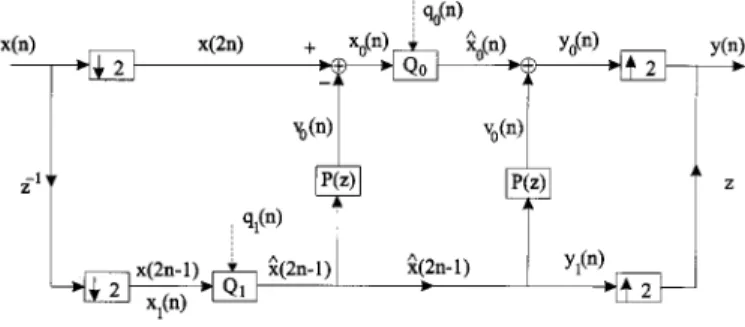
Consider Fig. 1. Note that the input to at the analysis end is , whereas the input to at the synthesis end is its quantized version . This means that in the recon-struction process, is added to the top branch through the filter . To avoid this, we can move the quantizer to the left, as shown in Fig. 2. This has the dramatic effect of making the noise gain unity. We will refer to Fig. 2 as the MINLAB coder. To explain the unity noise gain property of this structure, note that from Fig. 2, we have
From the above equations and Fig. 2, we can conclude that the errors on the top and bottom branches are, respectively
Therefore, the average variance of output error in the MINLAB coder is given by
The above equation is valid for any additive noise source. We
do not make any assumptions on and . That means, the noise gain is always one, even though the FB is never or-thonormal. If the quantizers used are scalar quantizers that sat-isfy (2), then the above expression for can be rewritten as (4) where we have used the fact that . Applying the arith-metic mean (AM) geometric mean (GM) inequality to the above equation and using (3), we get
with equality if and only if the bits are allocated as
(5)
Equal Stepsize Rule: From the above derivation, we see that
the average output noise variance is minimized when the two quantizers have the same noise variance. The noise vari-ances and the quantization stepsize are related as
. Therefore, we conclude that the MINLAB coder continues to be optimal if the stepsizes of the quantizers are equal.
Coding Gain: If we define the coding gain of the coder as the
ratio of the error variance in direct quantization [as in (2)] over that of the coder , then under the optimal bit allocation (5), the coding gain can be written as
(6)
A. Optimal Biorthogonal Coders
In this subsection, we will find such that the coding gain in (6) is maximized. We will first consider the FIR case and then the IIR case.
1) Optimal FIR MINLAB Coder: From (6), the coding gain
is maximized if is minimized. The optimal solution of , such that is minimized, can be obtained from linear prediction theory [25]. To see this, let be an FIR filter of the form
(7)
Then, the optimal solution is precisely the optimal predictor of based on the observations of
. The noncausal predictor can
Fig. 2. MINLAB encoder and decoder.
be used here since we are predicting the even samples from the odd samples. A causal implementation of such a system is al-ways possible by inserting enough delays at appropriate places in Fig. 2. Let be a real-valued WSS process with autocorre-lation coefficients . Then, using the orthogonality principle [18], [25], the optimal that minimizes is the solution of
(8) where the matrix and the vectors are as shown by at the top of the next page. Note that the matrix above is the autocorrelation matrix of the signal , and hence, it is positive definite (except for the special case when is a line spectral process). Therefore, the above normal equation can be solved in by using the Levinson fast algorithm. The optimal predictor is given by
(9) In addition, the minimum achievable variance is given by
(10)
and the prediction gain is
(11) The above inequality follows from the linear prediction theory [25]. The prediction gain is unity if and only if all the observa-tions are uncorrelated to the target of prediction . In this case, the optimal bit allocation formula in (5) reduces to
Therefore, the better the prediction is, the more bits are assigned to , and the fewer bits are assigned to . The coding gain in (6) then becomes . Note that in the derivation of (8), we have assumed that the autocorrelation matrix of the quantized observations is very close to that of the original observation. This assumption is valid only when the bit rate is high so that the quantization noise variance is small. In the case of low bit rate coding, the autocorrelation matrix of can differ significantly from that of . This can result in a substantial loss in coding performance. In next
.. . ... ... . .. ... ... .. . .. .
section, we will show how to obtain the minimum mean-square-error (MMSE) predictor.
Linear-Phase Property: The optimal predictor obtained from solving (8) has linear phase, i.e., . To see this, note that the matrix on the left-hand side of (8) satisfies
where is the reversal matrix of size , as defined in Sec-tion I. Since the vector is symmetric, we have . Using these properties and the fact that , we can rewrite (8) as
Comparing the above equation and (8), we conclude that . The vector is symmetric and hence has linear phase. Summarizing all the results, we have
Theorem 1: Consider the MINLAB coder in Fig. 2, where
is as in (7). The coding gain of the coder is maximized when is chosen as the optimal prediction filter in (9). The optimal prediction filter has linear phase, and the maximum coding gain is given by
where is the prediction gain in (11). The coding gain is al-ways greater than or equal to unity with equality if and only if the autocorrelation coefficients of satisfy
for .
2) Optimal IIR Biorthogonal Coders: The pre-dictor can be taken as the more general IIR filter. The predictor can be optimized such that is minimized. The special case when is an allpass filter is studied in [24]. It was shown that for a wide class of random process, a first-order IIR prediction filter provides satisfactory coding results. To be more specific, the prediction filter is taken as a first-order allpass function
The analysis filter in (1) becomes
. IIR filters of this form are studied in detail in [4], and it was shown that they have many good features. For
example, they always have at least one zero at . In this case, the variance of has the form [26]
To get the optimal IIR predictor, we can find such that the above quantity is minimized. If the input is a MA(1) precess, then . If the input is an AR(1) process, then
[26].
B. Connections and Comparisons with Other Coding Systems Comparison with DPCM: The differential pulse coding
mu-dolation (DPCM) is also a prediction-based coding technique. The coding gain of a DPCM system is the prediction gain. The proposed biorthogonal coder differs from DPCM in a number of ways.
1) In DPCM (either open-loop or closed-loop), the decoding process always involves a feedback path. In the MINLAB coder, the reconstruction process uses only FIR filter if
is FIR.
2) In DPCM, the predictor can only make use of the past data for prediction. In the MINLAB coder, the predictor can use past and future data for prediction. Hence, in (11) can be larger than the prediction gain in DPCM. That means, for certain inputs, the coding gain of the biorthog-onal coder can be larger than that of a DPCM of the same complexity, as we will demonstrate in Section VI-B. 3) The optimal predictor in a DPCM system has minimum
phase and, hence, cannot be linear phase. On the other hand, the optimal filter in the MINLAB coder always has linear phase for real-valued WSS processes. Moreover, the predictor is working at half of the input data rate. Therefore, the complexity of the MINLAB coder is about one fourth that of DPCM with the same prediction filter length.
4) Unlike DPCM, the MINLAB coder has a hierarchical structure. Therefore, progressive resolution transmission can be done, and coding schemes like the zerotree algo-rithms [15] and [27] can be used to further exploit the correlation among different scales.
A Very Low Delay Coder: In many applications such as
speech coding, we need coders with low delay. To obtain a low delay coder, we can take the filter as a causal FIR filter of the form . Then, a causal implementation of Fig. 2 can be obtained by replacing the advanced chain by a
delay chain. In such a causal implementation of Fig. 2, regard-less of the filter length , the coder has a delay of only one sample (i.e., ). The optimal solution of is the given by the optimal causal predictor of based on the
observations .
Connection to the Optimal Orthonormal Coder: It was shown
in [23] and [24] that the optimal FIR orthonormal coder (with order ) has a unity coding gain if and only if the au-tocorrelation coefficients of the input satisfy
for . Comparing this result with Theorem 1, we conclude that the optimal biorthogonal coder has a unity coding gain if and only if the optimal orthonormal coder of the same order has a unity coding gain. In fact, for most inputs, the biorthogonal coder outperforms the orthonormal coder, as we will see in Section VI.
Connection to the KLT: It is known that the Karhunen-Loeve
transform (KLT) for the two-channel case has the form
and the coding gain of the KLT is given by
For the proposed biorthogonal coder, if we take the filter , then we call the coder a biorthogonal transform. The op-timal predictor will be , and the coding gain for the biorthogonal transform is identical to .
IV. MMSE PREDICTIONFILTER FORQUANTIZEDOBSERVATION SAMPLES
With high bit rate assumption, . The
optimal predictor in Section III is designed based on unquan-tized observations . In this section, we will derive the MMSE predictor by taking into account that the observation samples are quantized data . We will assume that the quantization noise is uncorrelated with the quantizer input. Let be the autocorrelation matrix of the quantization noise . Following steps similar to those in Section III, we can derive the optimal MMSE predictor
(12) where and are defined in (8). The matrix con-tinues to be positive definite and Toeplitz, and the optimal so-lution in (12) can be obtained by the Levinson fast algorithm.
Moreover, . Therefore, the MMSE
prediction filter also has linear phase. To carry on the derivation, we will assume that the quantization noises and are uncorrelated, and their variances are equal (this is a reasonable assumption as the stepsizes of the quantizers are equal)
To further simplify (12), we need the matrix inversion formula
where and are nonsingular matrices of the same dimension. Applying the above identity to (12), we have
(13) where is the optimal predictor in (9). Recall that is the optimal predictor when the observation samples used are unquantized original data . In the case of quantized observation samples, the optimal predictor has a correction term proportional to . In the case of high bit rate coding, this term will be insignificant, and . From (13), we can verify that the MMSE is given by
(14) where is the prediction error variance for the case of unquan-tized observation in (10). Since the matrix is a positive definite matrix, we have for all . Therefore, the prediction error variance increases if the obser-vation samples are the quantized data. This increase is propor-tional to the quantization error variance . This explains why the coding gain of MINLAB decreases as the bit rate decreases.
1) Comparison of Performances of the Predictors in (8) and in (12) for Coarse Quantization: Consider the case when the
predictor used is but the observation samples are in fact the quantized data. Therefore, there is a mismatch between the predictor and its observation samples. In this case, we can show that the error variance is
Note that the amount of increase due to the mismatch is pro-portional to the quantization error variance and the prediction filter's energy. When the data are quantized coarsely, can become the dominant term, and the prediction error
can even be larger than the orignal signal (a prediction loss). The performance of the predictor can degrade significantly at low bit rate coding.
Comparing the above equation with (14), we have
Since the matrix is positive definite, the difference for any nonzero predictor. In fact, we can verify that this difference is bounded by
where and are, respectively, the maximum and min-imum eigenvalues of . We see that when the quantization error is large, the increase of prediction error caused by the mis-match of the predictor and the observation data can become very significant. Therefore, it is important to design a predictor that matches the observation samples, especially at low bit rate coding.
V. MERITS OF THEMINLAB CODER
The MINLAB coder in Fig. 2 enjoys many advantages. It has many other good features that make it attractive in various applications. In the following, we list some of its advantages.
1) Structurally PR: Similar to the orthonormal FB, the pro-posed biorthogonal FB has a structurally PR implemen-tation, as in Fig. 2.
2) Equal stepsize rule: Like the orthonormal coder, the equal stepsize rule is an optimal quantization procedure, as discussed in the last section. Entropy coding can be applied to further compress the quantizer output. 3) Unity noise gain: The synthesis bank does not amplify
the quantization noise. Hence, the optimal MINLAB coder has a coding gain . Moreover, we will show later that for two important classes of inputs [that is, the AR(1) process and MA(1) process], the optimal MINLAB coder with two taps outperforms the optimal orthonormal coder of any order.
4) Low design cost: The design of the optimal MINLAB coder is simple. Unlike the optimal orthonormal coder, neither constrained optimization nor spectral factoriza-tion is needed. Optimal MINLAB coder can be obtained by using Levinson algorithm.
5) Low complexity: To implement the analysis or synthesis bank, we need only one filter . Moreover, the op-timal has linear phase. Therefore, the complexity of the biorthogonal coder is roughly one fourth that of an orthonormal coder of the same order.
6) Coding gain increases with : It is well-known that the prediction gain is a nondecreasing function of . Hence , the coding gain increases when the filter order increases.
7) Low delay: It is known that the delay of an orthonormal coder is proportional to the filter order [18]. The longer the filters are, the larger the system delay is. In the MINLAB coder, if is a causal filter (either IIR or FIR), then the system delay is only one sample, regard-less of the filter order. As the prediction gain increases with filter order, so does the coding gain. Therefore, we can improve the performance of such a biorthogonal coder without introducing extra system delay.
8) Lossy/lossless compression: Let the input be a dis-crete amplitude signal with stepsize . For many ap-plications, the inputs are integers, and . Suppose the output of is quantized using a quantizer . Then, the MINLAB coder can be modified for lossless compression as follows.
a) Set the stepsize of . Any type of quantizer (round off or truncation or ceiling) can be used as .
b) Set the stepsizes of the subband quantizers as . Use entropy coding to encode the outputs of and .
When , we have a lossy MINLAB
coder. It becomes lossless when . 9) Coding of finite length signal: In a conventional
sub-band coder, when the input has finite length , the total
number of samples in the subband increases due to linear convolution with the analysis filters, unless these filters have length 2. Therefore, periodic extension is used to solve this problem. In the MINLAB coder in Fig. 2, to reconstruct the output signal, we need only to re-tain samples in the subbands [ samples
of and samples of where
de-notes the largest integer ]. No periodic extension is needed. To see this, let us ignore the quantizers in Fig. 2. It is clear that has nonzero
samples, and has nonzero samples.
Note that . Therefore, to reconstruct , we need to retain only samples of . Moreover, since
for , we need to retain only the first samples of for the reconstruction of .
10) Incorporation of EZW and SPIHT algorithm: As we will see in Section VII, the MINLAB coder in Fig. 2 can be generalized to obtain a tree structure MINLAB coder. Such a system continues to enjoy all of the properties listed above. Using this wavelet-type MINLAB coder, zerotree algorithms such as EZW and SPIHT [15], [27] can be applied.
VI. PERFORMANCEANALYSIS
In this section, we will provide several examples to demon-strate the coding performance of the proposed biorthogonal coder. The results will be compared with the optimal or-thonormal coder.
A. AR(1) Inputs
Let the input be an AR(1) process with for . For this AR(1) process, we compare the performance of the following various coders:
1) Let . From the normal equation (8),
we get the optimal predictor as .
In this case, the optimal coding gain has the closed-form expression
where the index 2 indicates that the predictor has two taps. In this case, however, only one multiplier is needed. We can verify that there is no need to use a longer predictor because the coding gain cannot be increased by using a longer filter. Therefore, the gain given in the above equation is the max-imum coding gain that can be attained by MINLAB coder with any prediction filter order.
2) Take . The optimal predictor is simply , and the coding gain is
3) Consider the coding gain for optimal orthonormal coders with infinite taps and four taps. It was shown in [22]–[24] that the coding gains are, respectively
4) The DPCM of order one is optimal in this case as the input is an AR(1) process. Its coding gain is given by
5) Suppose that we use the traditional biorthogonal coder in Fig. 1. Then, it can be shown that the maximum achievable coding gain for a two-tap filter is given by
where
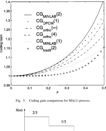
These gains are shown in Fig. 3. It is clear from the figure that
for all possible . Therefore, we see that for AR(1) process, the optimal MINLAB coder with two taps (one multiplier) outperforms the optimal orthonormal coder with infinite number of taps. From Fig. 3, we also note that for the traditional biorthogonal coder in Fig. 1, its coding
gain for .
We also compare the performance of the MINLAB coder with the widely used filters. Fig. 4 shows that the coding gain of MINLAB coder has a higher coding gain for AR(1) process with all . In other words, the MINLAB coder has a better decorre-lation ability than the filters. The MINLAB coder has only two taps (one multiplication), whereas the filters have 16 taps (eight multiplications). However, the filters are signal independent, whereas the MINLAB coder is signal dependent.
B. MA(1) Inputs
Let the input be an MA(1) process with ,
for , and for all the other . Then, the op-timal prediction filters of two taps and one tap are, respectively, and . The coding gain for these two biorthogonal coder are, respectively
Note that in this case, there is no need to use a predictor longer than two taps. The coding gain cannot be increased by using a longer filter [this can be seen from the normal equation (8)]. Therefore, above is the maximum coding gain that can be attained by MINLAB coder with any prediction filter order. For optimal orthonormal coder, it was shown [23], [24] that the coding gain is
Fig. 3. Coding gain comparison for AR(1) process.
Fig. 4. Comparison of MINLAB coder and the9=7 filters for AR(1) process.
For the DPCM with one multiplier, its coding gain is
The coding gain for the traditional coder in Fig. 1 is
From these coding gain expressions, it is not difficult to prove that
Fig. 5. Coding gain comparison for MA(1) process.
Fig. 6. Example of piecewise constant spectrum.
for all . The optimal MINLAB coder with two taps again outperforms than the optimal orthonormal coder. More-over the optimal MINLAB coder with two taps (one multiplica-tion) is superior to the DPCM with one multiplication. All these gains are shown in Fig. 5.
C. Inputs With
For orthonormal coders, the coding gain is independent of the even autocorrelation coefficients [22]. In this subsection, we consider the case when the input is a WSS process with its autocorrelation coefficients satisfying . One example that satisfies this condition is shown in Fig. 6. Since
, we have , and we have .
Therefore, the optimal predictor in (9) has the closed form
(15) It is shown in Appendix A that the variance of can be expressed as
(16) Using Theorem 1, the coding gain of the MINLAB coder is
(17)
Fig. 7. Traditional tree structure subband coder using ladder. where the argument indicates that there are infinite number of taps. If is a Gaussian process, then the rate distortion theo-retic bound [28] on the coding gain of any compression system is given by (see Appendix B)
(18)
This rate distortion theoretic bound can be achieved by DPCM of infinite order [25]. Using the fact that for any non-negative function (with equality if and only is a constant), we can conclude from (17) and (18) that
and can be achieved by the MINLAB coder if and only if the product is a constant. For the optimal orthonormal coder with an infinite order, it is shown
[22] that achieves in (18) if and only
if and is a constant.
There-fore, both the and achieve the
rate distortion theorectic bound for the same class of spec-trum. For the example shown in Fig. 6, we can verify that
. VII. TREESTRUCTUREMINLAB CODERS
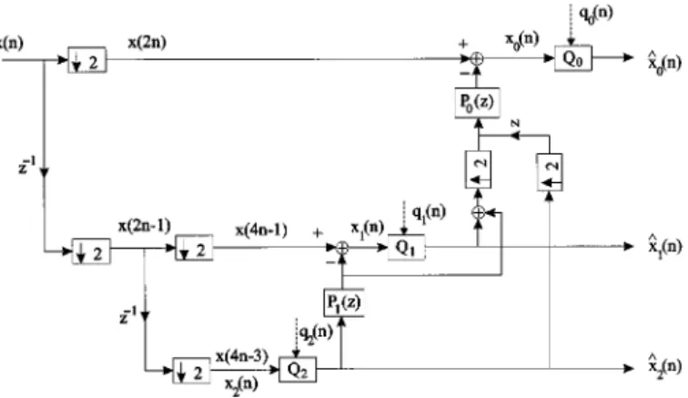
In the MINLAB FB shown in Fig. 2, the energy is mostly in the lower branch. Therefore, we decompose the lower sub-band signal to obtain a biorthogonal wavelet decompo-sition, as shown in Fig. 7. In a traditional wavelet coding, the quantizers are placed directly after the subband signals as in Fig. 7. There will be a mismatch between the encoder and de-coder. At the encoder, the inputs to and are the orig-inal data, whereas at the decoder, the inputs to and are the quantized data. It can be verified that this mismatch will cause the amplification of quantization noise in the reconstruc-tion process. In the following, we will introduce a minimum noise structure with unity noise gain for the ladder-based tree structure biorthogonal coder. We will first derive the results for the two-level decomposition in Fig. 7, and then the results of the more general -level decomposition will be stated without proof.
A. Two-Level Tree Structure MINLAB Coder
To avoid mismatch, we can use the quantized data as the input to and at the encoder. This can be done by modi-fying the encoder as in Fig. 8. Using an analysis similar to the
two-channel case, it can be shown that the following relations continue to hold:
Therefore, the average output noise variance is given by
(19) where we have used (2) and the fact that . The average bit rate in this case is
Using the above equation and applying the AM-GM inequality to (19), we have
where
(20) with equality if and only if the bits are allocated as
Note that there is no feedback loop in the minimum noise struc-ture shown in Fig. 8. Therefore, stability is always guaranteed.
Optimizing the Filters and : Let and be FIR filters of the form
From (20), the lower bound is minimized if and are designed to minimize and , respectively. To mini-mize the variance of , the filter is chosen as the op-timal predictor obtained in Section III. To minimize the variance of , the filter is designed as the optimal predictor of
based on the observations of
. The optimal solution of can be obtained from a normal equation similar to (8). We can show that both and have linear phase. The predic-tion gains of these filters are
The inequalities follow from linear prediction theory. The gain if and only if the autocorrelation coefficients
for . The gain if and only
if for . Under the optimal bit
allocation, the coding gain is given by
Fig. 8. Tree structure MINLAB encoder. Its decoder is the same as that in Fig. 7.
Therefore, the maximum coding gain of the two-level MINLAB coder in Fig. 8 is never less than that of the one-level MINLAB coder in Fig. 2.
B. -Level Tree Structure MINLAB Coder
The same idea can be extended to the more general -level tree structure FB. If the inputs to all the prediction filters at the encoder are quantized data, the noise gain will be unity, and such a -level tree structure will have the minimum noise property. Since all the derivations are very similar to the two-level decomposition, we will simply state the results below.
Let be the prediction gain of the predictor at the th level. Then, the optimal bit allocation formula becomes
In addition, under the optimal bit allocation, the coding gain is (21) Since all , we conclude that the coding gain is unity if and only if all of the prediction gains are unity. Moreover, the coding gain satisfies the recursive formula
where is the coding gain of a -level tree structure FB. Therefore, the coding gain always improves when we increase the number of levels. However, the coding gain saturates as increases, as we will see in the example at the end of this section.
Comments on the Complexity: If the predictor is chosen as , then the optimal predictors will have linear phase. To implement one level of the MINLAB encoder, we need to implement one linear phase predictor and two adders (except for the th level, which needs only one adder). There-fore, the complexity of an th-level MINLAB encoder is that of and additions. Comparing the non-MINLAB en-coder with traditional structure in Fig. 7, the MINLAB enen-coder needs more additions. The complexity of decoder for both cases is the same.
Asymptotic Results as Approaches Infinity: Let
. We will study the asymptotic results of this ideal case as the number of level approaches infinity.
Fig. 9. Coding gain of tree structure MINLAB coder.
From Theorem 1, we know that if and only if the autocorrelation coefficients satisfy for all
. By using
it is not difficult to see that the coding gain of a -level ideal
MINLAB coder satisfies if and only if
the input signal is white.
Example: Let the input be an AR(1) process with . Using the normal equation (8), we can get the prediction gain of the predictor as
Substituting this result into (21), the coding gain of an -level is
This coding gain is plotted in Fig. 9 for three different values of . Compared with the case of the one-level MINLAB in Fig. 2, the coding gain of the two-level or three-level MINLAB coder is much larger. In addition, note that the coding gain sat-urates as the number of levels increases. The saturation point depends on the correlation of the data. For AR(1) process,
for , respectively.
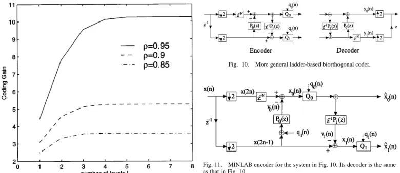
VIII. A MOREGENERALMINLAB CODER
The biorthogonal coder in Fig. 2 uses only one ladder. Such a system is a special case of the more general biorthogonal FB shown in Fig. 10. The FB in Fig. 10 is studied in detailed in [4]. In the simple coder of Fig. 2, only the variance of the even sam-ples is reduced by prediction from odd samsam-ples, but the variance
Fig. 10. More general ladder-based biorthogonal coder.
Fig. 11. MINLAB encoder for the system in Fig. 10. Its decoder is the same as that in Fig. 10.
of the odd samples is unchanged. Hence, its performance is lim-ited by the lower branch of Fig. 2. In the following, we will show how to apply the more general structure of Fig. 10 to reduce the variance of .
In this section, we assume that the filters and are causal filters of the form
The choice of and will be discussed later in the design. Note that the filter on the second ladder is
instead of . This delay is inserted so that there will be no delay-free loop in the MINLAB structure. For the coder in Fig. 10, its minimum noise structure is shown in Fig. 11. In the minimum noise structure, the quantization noise is added to the first ladder so that the input to is the quantized data . Since depends only on the past values of , we do not have a delay-free loop. To see why the noise gain is unity for the MINLAB coder, we can carry out the following analysis. From Fig. 11, we have
From the above equations, we get
and . The noise gains for
the upper and lower branch are both unity. By carrying out the similar derivation as in Section III, we can verify that the coding gain is maximized if the product is minimized, and the maximized coding gain can be expressed as
Designing the Predictors to Maximize the Coding Gain in
(22): From Fig. 11, it is clear that depends only on , whereas depends on both and . To find the global optimality, we need nonlinear optimization. Therefore, we consider a suboptimal solution. Since depends only on , we can design to be the optimal predictor of
. After designing , the subband signal is known. Its autocorrelation coefficients and its cross correlation coefficients with can be calculated. Using this information, the optimal predictor can be derived from the normal equation. Note that we are using the residue of the even samples for prediction of . In general, the choice of and will affect the coding gain. One way to decide these parameters is the following.
1) Choice of : Note that we are using the odd samples
on the two sides of for the prediction of . To get a linear-phase filter , we can
choose .
2) Choice of : When increases, the prediction gain of increases. However, the correlation between the observation and the target typically be-comes weaker as grows. The prediction gain of decreases as increases. Therefore, there is a tradeoff between the gains of the two predictors and . 3) Choice of : As increases, the prediction gain of increases, but the complexity also grows. Note that in general, is not linear phase.
A Note on the Stability Issue: Note that there is no feedback
loop in the minimum noise structure in Fig. 11. The system is stable if both and are stable filters. We can verify that the noise transfer matrix from the quantizers to the subbands has the form
The noise tranfer matrix is FIR. Moreover, its determinant is unity. Hence, it is a unimodular matrix, and its inverse is also FIR.
IX. CONCLUDINGREMARKS
In this paper, we have proposed a minimum noise structure (Fig. 2) for the class of ladder-based FB. The coding perfor-mance of the proposed biorthogonal coder is analyzed in de-tail. For both AR(1) process and MA(1) process, the optimal biorthogonal coder with two taps (with a complexity of only one multiplication) outperforms any optimal orthonormal coders. In addition to its excellent coding performance, the coder has many other desired features (see Section V). These features make the biorthogonal coder a potentially valuable and attractive alter-native to the orthonormal coder. We have also generalized the minimum noise structure to the following two cases: 1) Tree structure biorthogonal FB and 2) more general biorthogonal FB with more than one ladder. In [29], we introduce a novel pre-diction-based lower triangular transform (PLT). The new trans-form is biorthogonal and has a minimum noise structure with unity noise gain. The PLT has an identical coding gain as the KLT, but it has a much lower design and implementation cost.
Given the input statistics, the PLT can be obtained by using the Levinson fast algorithm. In the special case of AR(1) process, the optimal biorthogonal transform coder has a closed-form ex-pression, and no optimization is required.
APPENDIX A PROOF OF(16)INEXAMPLE1
Since is given in (15), the analysis filter in (1) becomes
where we have used the fact that .
Com-paring the above equation with the power spectrum
, we have .
Since the downsampler does not change the variance, the minimum variance of can be expressed as
(23)
Since , we have for all
. Using this relation and the fact that is periodic, we can further simplify (23) as
APPENDIX B
THERATEDISTORTIONTHEORETICBOUND
For a Gaussian WSS process with power spectrum , the minimum distortion that can be achieved by any -bit coding system is given by [28]
To obtain the coding gain of the form in (18), we carry out the derivation
ACKNOWLEDGMENT
The authors are thankful to Prof. T. Q. Nguyen, Boston Uni-versity, Boston, MA, for bringing our attention to the recent de-velopments on lifting schemes, which inspired this work.
REFERENCES
[1] T. Endoh and Y. Tamazaki, “Progressive coding scheme for multi level images,” in Proc. Picture Coding Symp., Tokyo, Japan, Apr. 1986, pp. 21–22.
[2] A. M. Bruekers and A. W. M. van den Enden, “New networks for perfect inversion and perfect reconstructions,” IEEE J. Select. Areas Commun., vol. 12, Jan. 1992.
[3] C. W. Kim and R. Ansari, “FIR/IIR exact reconstruction filter banks with applications to subband coding of images,” in Proc. Midwest CAS
Symp., Monterey, CA, May 1991.
[4] S.-M. Phoong, C. W. Kim, P. P. Vaidyanathan, and R. Ansari, “A new class of two-channel biorthogonal filter banks and wavelet bases,” IEEE
Trans. Signal Processing, vol. 43, pp. 649–665, Mar. 1995.
[5] C. W. Kim and R. Ansari, “Subband decomposition procedure for quin-cunx sampling grids,” in Proc. SPIE-Visual Commun. Image Process., Boston, MA, Nov. 1991.
[6] W. Sweldens, “The lifting scheme: A custom-design construction of biorthogonal wavelets,” Appl. Comput. Harmon. Anal., vol. 3, no. 2, pp. 186–200, 1996.
[7] W. Sweldens, “The lifting scheme: A construction of second generation wavelets,” SIAM J. Math. Anal., vol. 29, no. 2, pp. 511–546, 1997. [8] I. Daubechies and W. Sweldens, “Factoring wavelet transforms into
lifting steps,” J. Fourier Anal. Appl., vol. 4, no. 3, pp. 247–269, 1998. [9] R. Claypoole, G. Davis, W. Sweldens, and R. Baraniuk, “Nonlinear
wavelet transform for image coding,” in Proc. 31st Asilomar Conf.
Signals, Syst., Comput., vol. 1, 1997, pp. 662–667.
[10] R. L. de Queiroz, D. A. F. Florencio, and R. W. Schafer, “Nonexpan-sive pyramid for image coding using nonlinear filterbank,” IEEE Trans.
Image Processing, vol. 7, pp. 246–252, Feb. 1998.
[11] P. Roos, A. Viergever, and M. C. A. van Dijke, “Reversible intraframe compression of medical images,” IEEE Trans. Med. Imag., vol. 7, pp. 328–336, Sept. 1988.
[12] G. R. Kuduvalli and R. M. Rangayyan, “Performance analysis of re-versible image compression techniques for high-resolution digital tel-eradiology,” IEEE Trans. Med. Imag., vol. 11, pp. 430–445, Sept. 1992. [13] A. Said and W. A. Pearlman, “Reversible image compression via mul-tiresolution and predictive coding,” Proc. SPIE, pp. 664–674, Nov. 1993. [14] W. J. Ho and W. T. Chang, “Multiresolution interpolative DPCM for data
compression,” Proc. SPIE Vis. Commun. Image Process., 1995. [15] A. Said and W. A. Pearlman, “An image multiresolution representation
for lossless and lossy compression,” IEEE Trans. Image Processing, vol. 5, pp. 1303–11, Sept. 1996.
[16] A. R. Calderbank, I. Daubechies, W. Sweldens, and B. Yeo, “Lossless image compression using integer to integer wavelet transforms,” in Proc.
IEEE Int. Conf. Image Process., 1997, p. 596.
[17] M. Iwahashi, S. Fukuma, and N. Kambayashi, “Lossless coding of still images with four channel prediction,” in Proc. IEEE Int. Conf. Image
Process., 1997, p. 266.
[18] P. P. Vaidyanathan, Multirate Systems and Filter Banks. Englewood Cliffs, NJ: Prentice-Hall, 1993.
[19] S.-M. Phoong and Y. P. Lin, “A new class of optimal biorthogonal coder,” IEEE Signal Processing Lett., vol. 6, pp. 4–6, Jan. 1999.
[20] S.-M. Phoong and Y. P. Lin, “Optimal ladder-based biorthogonal coder,” in Proc. IEEE Int. Conf. Acoust. Speech, Signal Process., Mar. 1999. [21] M. K. Tsatsanis and G. B. Giannakis, “Principle component filter banks
for optimal multiresolution analysis,” IEEE Trans. Signal Processing, vol. 43, pp. 1766–1777, Aug. 1995.
[22] P. P. Vaidyanathan, “Theory of optimal orthonormal coder,” IEEE Trans.
Signal Processing, vol. 47, pp. 1528–1543, June 1998.
[23] A. Kirac and P. P. Vaidyanathan, “Theory and design of optimal FIR compaction filters,” IEEE Trans. Signal Processing, vol. 47, pp. 903–919, Apr. 1998.
[24] J. Tuqan and P. P. Vaidyanathan, “Globally optimal two channel FIR orthonormal filter banks adapted to the input signal statistics,” presented at the the IEEE Int. Conf. Acoust., Speech Signal Process., 1998. [25] J. Makhoul, “Linear prediction: A tutorial review,” Proc. IEEE, vol. 63,
pp. 561–580, 1975.
[26] J. Tuqan and P. P. Vaidyanathan, “Optimum low cost two channel IIR or-thonormal filter bank,” in Proc. IEEE Int. Conf. Acoust., Speech, Signal
Process., Apr. 1998, pp. 2425–2428.
[27] J. M. Shapiro, “Embedded image coding using zerotrees of wavelets,”
IEEE Trans. Signal Processing, vol. 41, pp. 3445–3462, Dec. 1993.
[28] T. Berger, Rate Distortion Theory. Englewood Cliffs, NJ: Prentice Hall, 1971.
[29] S.-M. Phoong and Y. P. Lin, “PLT versus KLT,” in Proc. Int. Symp.
Cir-cuits Syst., May 1999.
See-May Phoong (M'96) was born in Johor,
Malaysia, in 1968. He received the B.S. degree in electrical engineering from the National Taiwan University (NTU), Taipei, Taiwan, R.O.C., in 1991 and the M.S. and Ph.D. degrees in electrical engi-neering from the California Institute of Technology (Caltech), Pasadena, in 1992 and 1996, respectively. He was with the Faculty of the Department of Electronic and Electrical Engineering, Nanyang Technology University, Singapore, from September 1996 to September 1997. Since September 1997, he has been an Assistant Professor with the Institute of Communication Engineering and Electrical Engineering, NTU. His interests include signal compression, transform coding, and filter banks and their applications to communications.
Dr. Phoong was the recipient of the 1997 Wilts Prize at Caltech for Out-standing Independent Research in Electrical Engineering.
Yuan-Pei Lin (S'93–M'97) was born in Taipei,
Taiwan, R.O.C., in 1970. She received the B.S. degree in control engineering from the National Chiao-Tung University, Hsinchu, Taiwan, in 1992 and the M.S. and Ph.D. degrees, both in electrical engineering, from the California Institute of Tech-nology, Pasadena, in 1993 and 1997, respectively.
She joined the Department of Electrical and Con-trol Engineering, National Chiao-Tung University, in 1997. Her research interests include multirate filter banks and applications to communication systems. Dr. Lin is currently an Associate Editor of the journal Multidimensional