基於多視角影像之戶外場景前景背景分離技術研究

國

立

交

通

大

學

電子工程學系 電子研究所

碩 士 論 文

基於多視角影像之戶外場景前景背景分離技術研究

A Study on Outdoor-Scene Foreground/Background

Separation over Multi-camera System

研 究 生：羅介暐

指導教授：王聖智 教授

基於多視角影像之戶外前景背景分離技術研究

A Study on Outdoor-Scene Foreground/Background

Separation over Multi-camera System

研 究 生：羅介暐 Student：Jie-Wei Lo

指導教授：王聖智 教授 Advisor：Prof. Sheng-Jyh Wang

國 立 交 通 大 學

電子工程學系 電子研究所

碩 士 論 文

A Thesis

Submitted to Department of Electronics Engineering and Institute of Electronics

College of Electrical and Computer Engineering National Chiao Tung University

in partial Fulfillment of the Requirements for the Degree of

Master of Science in

Electronics Engineering

August 2013

Hsinchu, Taiwan, Republic of China

i

基於多視角影像之戶外場景前景背景分離技術研究

研究生：羅介暐 指導教授：王聖智 教授

國立交通大學

電子工程學系 電子研究所碩士班

摘要

在影像分割的技術中加入少量的使用者自定義的前後景仍然難以在複雜環境下 切割出完美的前景物，而對於全自動的前景物切割，建立背景模型便是我們的 第一步。在本篇論文中，我們著重在即使在戶外的複雜環境，仍然可以用低成 本的系統去自動的達到前景背景分離的技術。首先，基於混合高斯背景模型， 再配合非線性色彩分佈和多視角影像的輔助，我們設計最佳化問題來得到初步 的前景物資訊，並且抵抗影子的影響，之後再利用影像分割的概念配合背景的 資訊和初步的前景資訊去得到最後切割完整的前景物。有了切割出來的前景 物，再配合人為的合成背景便可以在戶外輕鬆得到室內虛擬攝影棚想要的效 果。實驗結果證明我們所提出的方法有許多前景分割的好處，其中包含全自動 化、移除影子的干擾和即便在戶外環境中也能得到完整而且邊緣平滑的前景 物。

ii

A Study on Outdoor-Scene Foreground/Background

Separation over Muti-camera System

Student：Jie-Wei Lo Advisor：Prof. Sheng-Jyh Wang

Department of Electronics Engineering, Institute of Electronics

National Chiao Tung University

Abstract

The state-of-art interactive image segmentation algorithms often have difficulty in correctly extracting the foreground objects from cluttered background with limited user’s guidance. For automatic foreground object detection, constrained background models are critical. In this thesis, we propose a low-cost automatic foreground/background separation system that can be applied to outdoor scenes. Based on a Gaussian mixture model, together with the inclusion of non-linear tone mapping and multi-view image constraint to further eliminate shadow effect, we formulate an optimization problem to deal with the foreground extraction problem by using more robust image features in the image matting technique.

The proposed method exhibits many desired properties of an effective foreground segmentation algorithm, including automatically extraction of foreground regions, the ability to produce smooth and accurate boundary contour, and the ability to handle severe color variations in an outdoor environment with relaxed background constraints. The whole system can achieve fully automatic foreground object extraction with satisfactory accuracy for a multi-camera system.

iii

致謝

在此特別感謝教授 王聖智老師的指導，在研究過程中，每週固定的進度報告裡給 予研究上的方向和改進，訓練我們如何分析問題、剖析並且解決，在表達方面也會叮嚀 我們如何用投影片和報告等方式去表達給其他人簡潔有力的觀念。除了研究方面老師在 平常生活中的互動也讓我們有如父親般的親切，甚至和學生們一同參與體育競賽，讓實 驗室不只是個工作的環境，更像一個家庭讓我們學習如何成長。和同濟方面，感謝禎宇 和家豪二位博班學長的意見和指導，讓我可以找出問題的癥結點，達到事半功倍的研究 成果；秉宸、政銘、姿婷和佳峻四位戰友們這二年來的實驗室生活也因為你們一同奮鬥， 讓我在研究和生活都有許多的支持和動力，每週固定的進度報告裡也都能一同討論，讓 我對自己的研究之外的知識也大有長進，知道更多不同的技術和解決方法。而學弟妹冠 廷、非凡、汝欣、振源、奕中和子銘們也因為有他們的加入讓實驗室充滿了活力，可以 在實驗室外一起運動打球，偶爾溫馨的聚餐也讓 Vision Lab 的凝聚力更強，也因為大 家的彼此扶持，讓我的研究路上是快樂沒有壓力的。當然背後最重要的就是我親愛的家 人們了，總是默默的支持著我，沒有給過我任何的壓力，想回家時總是有滿滿的盛宴等 著我，即使只待一晚甚至只吃一餐，也都可以讓我的心力充滿能量勇往直前，一路上的 陪伴，才能有今天的我，感謝你們。

iv

Content

Chapter 1 Introduction ... 1

Chapter 2 Related Works ... 3

2.1 Single-View Foreground Extraction ... 3

2.1.1 Background Modeling ... 3

2.1.2 Interactive Image Segmentation ... 4

2.2 Multi-View Foreground Extraction ... 8

Chapter 3 Proposed Algorithm ... 13

3.1 Background Modeling ... 14

3.2 Spatial Consistency for multi-view ... 15

3.3 Convex Active Contour Model ... 21

3.3.1 Region Term Formulation ... 21

3.3.2 Boundary Term Formulation ... 25

3.4 Image Matting Model ... 28

3.5 Shadow Removed ... 31

Chapter 4 Experimental Results ... 36

Chapter 5 Conclusion ... 44

v

List of Figures

Figure 2-1 Classical Chroma-keying Environment……….… ...4

Figure 2-2 Image Matting (a) Manually selected scribbles. (b) Matting result based on (a) ….5 Figure 2-3 Color variation in outdoor scene (a) Original image. (b) Manually selected scribbles. (c) Matting result based on (b). (d) Zoom in of (c)……….… ....6 Figure 2-4 Color similarity between foreground and background. (a) Original image. (b) Manually selected scribbles. (c) Matting result based on (b). (d) Zoom in of (c)…….…7 Figure 2-5 Segmentation by stereo-pairs. (a) input left view (b) input right view (c) data(left image) (d) Segmentation based on stereo (e) segmentation based on color (f) The method fuses color, contrast and stereo to achieve a more accurate segmentation……..9 Figure 2-6 Result of silhouette extraction algorithm. (a) Input images. (b) Segmentation. (c) Output silhouettes………...………..… 10 Figure 2-7 Flow chart of Wonwoo et al. in [18]. Iteratively update background and foreground model parameters and segmented each image in a subsequent ste………..…. 12 Figure 3-1 Flowchart of our algorithm……….……….…13 Figure 3-2 Comparison the foreground detection. (a) Original image. (b) Foreground detection from directly subtraction. (c) Foreground detection from GMM backgroudn modeling.. ………...15 Figure 3-3 Traditional way to eliminate background noise by using morphology operator.(a) GMM background modeling of Figure 2-3(a). (b) Denoise by morphology operator result of (a). (c)Zoom in of (a). (d)Zoom in of (b)……….… ... 16 Figure 3-4 Epipolar Geometry (a) Image pair with fundamental matrix related to a point mapping to other image is a line (b) input image (view 1) (c) input image (view 2. ... 18 Figure 3-5 Multi-view constraint for denoising (Take view 4 for reference view). (a) Camera postion. (b) View 1 (c) View 2 (d) View 3 (e) View 4 (f) View 5 (g) View 6 (h) GMM modeling of (b). (i) GMM modeling of (c).(j) GMM modeling of (d). (k) Denoise of (h). (l) Denoise of (i). (m) Denoise of (j). (n) Viewing-ray interaction. (o) Output of multi-view constraint. ……….… .... ……….… 19 Figure 3-6 Multi-view constraint for denoising (Take view 4 for reference view). (a) Camera postion. (b) View 1 (c) View 2 (d) View 3 (e) View 4 (f) View 5 (g) View 6 (h) GMM modeling of (b). (i) GMM modeling of (c).(j) GMM modeling of (d). (k) Denoise of (h). (l) Denoise of (i). (m) Denoise of (j). (n) Viewing-ray interaction. (o) Output of multi-view constraint. …….……….… .... ……….…20 Figure 3-7 MTM distance measure between input image and background image patch by patch. (a) background image. (b) input image……….……….. ... 22 Figure 3-8 The MTM distance measure map. (a) Original image (b) Search entire image with window size 300 (c) Search entire image with window size 200 (d) GMM mask through

vi

multi-view constraint and simple morphology operator (e) MTM measure of (d) with

window size 300. (f) MTM measure of (d) with window size

200………….………24 Figure 3-9 The MTM distance map. (a) MTM measure of Figure 3-5(o). (b) MTM measure of Figure 3-6(o)…...………...……….… ... ……….… 25 Figure 3-10 Comparison of the results with and without |𝑟(𝒙)| in edge detection function.

(a)Result using |𝑓(𝒙)| . (b) Result using |𝑟(𝒙)| . (c) Result using Eqaution (3-6)………..………...27 Figure 3-11 Result of active contour output. (a) Active contour output of Figure 3-5 (o). (a) Active contour output of Figure 3-6 (o)………. ... 27 Figure 3-12 Image matting model………. ... 28 Figure 3-13 Automatically generated tri-map based on active contour model. …………... 29 Figure 3-14 Modified ML comparison. (a) Original matting result. (b) Modified ML result. . 30 Figure 3-15 Shadow eddect in synthesized image caused contrived result. ………….…. ... 31 Figure 3-16 Homography constraint show that a pixel in one view are warping to another view by a reference plane (ground)………. ... 32 Figure 3-17 Shadow detection. (a) Shadow on the ground. (b) MTM distance measure. ... 33 Figure 3-18 Shadow removed result………. ... 34 Figure 3-19 Multi-view constraint with shadow detection. (a) Original image. (b) GMM modeling of (a). (c) Multi-view constraint with shadow removed………. ... 35 Figure 4-1 More results on other camera views. (a) Original image. (b) Multi-view constraint. (c) Result of convex active contour model. (d) Result of modified image matting method ………...36 Figure 4-2 Comparison between the supervised image matting method and the proposed automatic method (a) Manually selected scribbles. (b) Synthesized image based on (a) and the original ML method. (c) Automatically generated tri-map. (d) Synthesized

image based on (c) and the modified ML

method………..……….37 Figure 4-3 Comparison between original ML and modified method. (a) Original ML method. (b)Modified ML method………...38 Figure 4-4 Compariosn of active contour model and image matting model. (a) Input image. (b) Active contour model. (c) Original image matting. (d) Modified image matting……..39 Figure 4-5 Compariosn of active contour model and image matting model. (a) Input image. (b) Active contour model. (c) Original image matting. (d) Modified image matting……..40 Figure 4-6 Compariosn of active contour model and image matting model. (a) Input image. (b) Active contour model. (c) Original image matting. (d) Modified image matting…….41 Figure 4-7 More result of the foreground object into the virtual scene………..43

1

Chapter 1 Introduction

Virtual studio, which can combine real actors or objects with synthesized scenes, is a powerful tool for the production of TV programs or movies. To generate seamless combination, accurate foreground extraction is the key. In many computer algorithms such as video editing, photo stitching, digital panoramas, space carving for 3D modeling, target tracking, and so on, extracting foreground region from background is the first requirement in single-view or multiple-view systems. A classical approach for foreground extraction is to build up a constrained background model which usually assumes the background is stationary without illumination changes. The foreground objects are then extracted by excluding the background regions. Chroma-keying approaches belong to this category and assume a uniform background, which is usually blue or green. Unfortunately, this kind of background modeling methods is usually limited to indoor environments. For an outdoor environment, how to maintain a consistent background model is much more complicated.

Video segmentation is another method to extract foreground regions [1]. This kind of methods detect moving object based on temporal difference of two consecutive frames, followed by a boundary fine-tuning process based on spatial information or temporal information. Several drawbacks exist in the change-detection-based approach. The detection results may have broken shape if the speed of the object moves fast in the video sequence. The poor quality of the segmentation process may not provide enough information for the following process, like object segmentation, tracking and recognition.

In order to achieve accurate foreground extraction, various supervised approaches have been proposed in the literature, such as Graph Cut-based methods [2], Random Walk method [3], Geodesic methods [4] [5] and Image matting method [6]. In these supervised approaches, foreground regions are identified by incorporating some additional guidance offered by the user. That is, the user has to define parts of the interested regions first. After that, these algorithms

2

formulate the foreground/background separation process as an optimization problem based on the guidance, together with some extra constraints over the image. Two popular image constraints are the smoothness constraint and the color consistency constraint. However, these supervised approaches may not always achieve satisfactory results in an outdoor environment, where the variations of color and lightness are far more complicated than that in an indoor environment.

In this thesis, we present an automatic foreground/background separation algorithm for a multiple-camera system. In order to deal with outdoor scenes, the proposed method adopts a non-linear tone mapping process to reduce the impact of illumination variations. Besides, we include the multi-view perspective to reduce the impact of background variations by combining foreground information from multiple images and use homography constraint to remove the shadow effect by assuming the shadow is shone on the ground. To further obtain smoother foreground boundaries, we adopt an active contour model to refine the foreground regions. Finally, we present a modified image matting method to derive finely carved foreground regions by including more robust image features into the computations of the matting affinity. The proposed framework can not only automatically identify the foreground objects for a multi-camera system but also accurately and effectively perform foreground/background separation in an outdoor scene with relaxed background constraints.

Important features of the approach are as follows: 1) robust to outdoor background and the final foreground region is smooth with precise boundary, 2) the proposed method is fully automatic and does not need the color consistency for foreground and background. In the latter case, cameras do not need to be color-calibrated since color consistency is not enforced among different viewpoints. This fact makes the proposed approach suitable for outdoor scenes.

The outline of this thesis is organized as follows. In Chapter 2, we review related works. In Chapter 3, the proposed framework is presented. Finally, in Chapters 4 and 5, experimental results and conclusions are given.

3

Chapter 2 Related Works

Many foreground extraction techniques have been proposed in the past few years. In this chapter, we will introduce some related work about foreground extraction. We will classify these works to single-view based and multi-view based foreground extraction techniques, depending on the number of camera views. In Section 2.1 and Section 2.2, some relevant works about single-view and multi-view foreground extraction will be introduced, respectively.

2.1 Single-View Foreground Extraction

In single-view based foreground extraction, there are two main classifications: background

modeling and interactive image segmentation. For background modeling, foreground regions

are extracted by assuming that the background model is known beforehand and by extracting foreground region which are different from the background model. In contrast, interactive image segmentation algorithm, which can separate the desired foreground from the background region by incorporating user’s involvement which defines some of the interested areas beforehand. Based on color similarity, the algorithm label the remaining pixels in the image to be either foreground or background. We will describe the details in the following sections.

2.1.1

Background Modeling

Background modeling is a way to separate foreground objects from the static background. In [7], Piccardi et al. have reviewed several popular approaches for background subtraction. These methods typically operate at the pixel level. A straightforward method is to directly subtract the static background image via median filtering or to take into account photometric information such as gray level, color space, texture, or image gradient. Chroma-keying approaches belong to this category which assume a uniform background that is usually green or blue, as shown in Figure 2-1.

4

Figure 2-1 Classical Chroma-keying Environment.

For non-uniform backgrounds, statistical models are usually used to describe the background model in order to deal with more complicated backgrounds. Statistical models are precomputed for pixels and the foreground pixels are then identified by comparing the current values to the model values. Several statistical models have been proposed for that purpose; for example, a non-parametric model [8] is proposed to identify cluttered or not completely static backgrounds. Normal distribution are used in conjunction with Mahalanobis distance or a mixture of Gaussian models is considered [21]. Other method use neural network based estimation [9]. These background subtraction methods have been widely used in the area of real-time surveillance system, although they require a learning step to obtain the knowledge of background color distribution.

2.1.2

Interactive Image Segmentation

Interactive image segmentation algorithms, which incorporates a small amount of user interaction to define the desired to-be-extracted contents, has received much attention in recent years. Many interactive image segmentation algorithms have been proposed in the literature. In general, interactive image segmentations can be classified into two categories: region-based approaches and boundary-based approaches. For example, some region-based approaches, like the Graph Cut-based methods [2], Random Walk method [3], Geodesic methods [4] [5] and the image matting method in [6], use iterative optimization to identify the foreground objects based

5

on user’s guidance. All these methods basically treat an image as a weighted graph with nodes corresponding to pixels in the image and edges being placed between neighboring pixels. They minimize a certain energy function on this graph to produce a segmentation result.

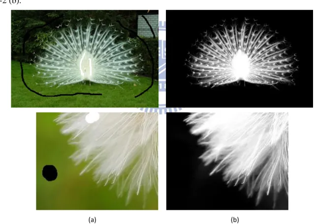
In interactive image segmentation, the user is often asked to draw two types of strokes to label some pixels as either foreground or background. After that the algorithm label all the remaining pixels. In Figure 2-2 (a), we show the manually selected scribbles for the image. In image matting, the algorithm compute every pixels with their affinity, or called similarity, as vertices to build up the whole graphical model. Based on the affinity, image decomposition is performed to get the final result that separates foreground from background as shown in Figure 2-2 (b).

(a) (b)

Figure 2-2 Image Matting (a) Manually selected scribbles. (b) Matting Result based on (a)

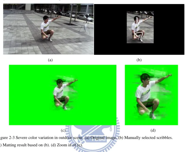
In image matting model, the affinity are computed by Matting Laplacian, which is usually computed only in the RGB color space. These approach are typically unsuitable for practical systems, such as surveillance cameras and outdoors scenes, because of severe color variations, such as sunlight change. An example shown in Figure 2-3, where the arm shone by sun is

6

brighter than the other parts of the arm. For this case, the matting result is pretty bad if with only a small amount of user input.

(a) (b)

(c) (d)

Figure 2-3 Severe color variation in outdoor scene. (a) Original image. (b) Manually selected scribbles. (c) Matting result based on (b). (d) Zoom in of (c).

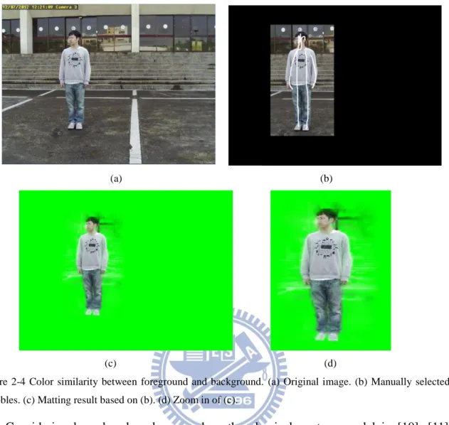
Another drawback of the original image matting method is the possible color similarity between foreground and background. The matting result will mix with background without smooth foreground boundary. An example is shown in Figure 2-4. If we only draw a small amount of user inputs to define foreground and background, the classification of the remaining pixels will be less accurate.

7

(a) (b)

(c) (d)

Figure 2-4 Color similarity between foreground and background. (a) Original image. (b) Manually selected scribbles. (c) Matting result based on (b). (d) Zoom in of (c).

Considering boundary-based approaches, the classical contour model in [10], [11] is originally proposed to segment the desired object by local contour adjustment to improve the smoothness of object boundary. Considering that the boundary-based approaches require great efforts to specify the boundary area or the boundary points, especially for complex shapes, most recent interactive image segmentation algorithms take regional information as the input. The active contour without edge model [12] adds in regional information and removes the dependency on edge detection. However, this method often gets dissatisfactory result due to non-convex modeling and may have local minima. Recently, the convex active contour proposed in [13] is able to find global optimize solution which can be generally formulized as:

min

0≤u≤1 (∫ 𝑔_Ω 𝑏|∇𝑢|𝑑𝑥 + 𝜆 ∫ ℎ_Ω 𝑟𝑢𝑑𝑥),

(2-1)

8

1) u(∙) is a function on the image domain Ω, whose value is constrained to the interval [0,1]. Once the optimal solution of Equation (2-1) is formed, the segmented region is found by thresholding the function u(∙) to get

Ω = {x|u(x) > T} (2-2)

2) Function gb(∙) is a non-negative boundary function. One common choice for the edge

detection function is

g_b(𝑥) = 1

1 + |∇𝐼(𝑥)|2 , (2-3)

where I(x) is the intensity of the image pixel x.

3) Function hr(∙) is a region function that measures the inside and outside of the

segmented region, as defined in [12].

By varying the tradeoff factor λ, we can balanced two terms called boundary term and region term in Equation (2-1). The boundary term ensures segmentation with boundaries along areas with smooth gradients. The second term favors the segmentation result that conforms with the object coherence criteria defined in function hr .

Several approaches have been proposed to solve Equation (2-1) for a given hr(∙). Recently,

Goldstein et al. [14] proposed to use the Split Bregman method to solve Equation 2-1. The Split Bregman method is a general solution for L1-regularized problem with convexity and is a much faster minimization method.

2.2 Multi-View Foreground Extraction

In a virtual studio, there are often several cameras to take images or videos. The aforementioned background subtraction methods and foreground object segmentation methods only address the foreground/background separation problem in a single image. However, foreground regions over different viewpoints should exhibit the same 3D zone region with spatial coherence. In other words, foreground regions over different viewpoints should exhibit

9

spatial coherence in the form of a common 3D space zone. In this section, we will introduce some approaches to extract foreground region in the multi-view perspect.

Early attempts has been made in [15], where depth information obtained from stereo images is combined with photometric information to segment foreground regions from background regions. Kolmogorov et al. in [15] proposed a real-time segmentation method that preserves the foreground object boundaries, under background changes, by combining stereo and color information. Incorporating depth information improves segmentation results over single camera view. As shown in Figure 2-5. Nevertheless, such methods are designed for short-baseline stereo systems and cannot easily be extended to multi-camera systems.

(a) (b)

(c) (d) (e) (f) Figure 2-5 Segmentation by stereo-pairs. (a) input left view (b) input right view (c) data(left image) (d) Segmentation based on stereo (e) segmentation based on color (f) The method fuses color, contrast and stereo to achieve a more accurate segmentation.

For multiple camera systems, there is some manner which exploits spatial coherence, or called silhouette coherence, through a spatial region instead of locally through pixel depths. Again, consistent foreground image regions give rise to a single 3D space region. Conversely, this region should project entirely on foreground regions in image domain; otherwise, it would

10

mean that there are space regions that correspond to foreground with respect to some viewpoints but correspond to background with respect to others. A few approaches exploit such a fact in various scenarios. Zeng and Quan [16] proposed intersection consistency and projection consistency by iteratively performing space carving with respect to the color consistency in each image. The result of [16] are shown in figure 2-6. This approach increases spatial consistency from one to another viewpoint; however, it only approximates spatial coherence, which should be enforced over all viewpoints simultaneously.

Figure 2-6 Results of Silhouette Extraction Algorithm: (a) Input images, (b) Segmentations, (c) Output silhouettes.

In another work, Sormann et al. [17] proposed graph cut based method to separate foreground from background. Spatial coherence is enforeced over different viewpoints by minimizing the difference between silhouette regions in two images at successive iterations. This approach uses color information, combined with shape prior got from multiple views, to

11

segment silhouettes with coherent shape. While improving over monocular approaches, this scheme relies on a strong assumption about the silhouette similarities between two neighboring views. This assumption is hardly satisfied even with small camera motion.

Wonwoo et al. [18] also use graph cut based method to extract foreground based on two assumption: 1) region of interest appears entirely in all images and 2) background colors are consistent in each image. That is, background colors are different from foreground colors but they are homogeneous over background pixels. They iteratively segment each image so that the background color satisfies color consistency constraints and all foreground regions correspond to the same space zone. To initiate this iterative process, Wonwoo exploits the first assumption to identify regions in the images that have to belong to background. Such background regions are the image regions that are outside the projection of the observation volume seen by all considered viewpoints. These initial regions are then grown iteratively by estimating each pixel’s occupancy based on its color and spatial consistency. This iterative operation can update foreground and background model parameters with latent variables. Denoting the remaining pixel belong to foreground or background, the image are segmented in a subsequent step using the new model parameters. The flow chart of their system is shown in Figure 2-7. Even through this approach outperforms these single-view approaches, this scheme relies on a strong assumption that is not suitable for wide-baseline systems.

12

Figure 2-7 Flow chart of Wonwoo et al. in [18]. Iteratively update background and foreground model parameters and segmented each image in a subsequent step.

Our primary motivation is to propose a method that automatically identifies foreground regions in several images without user’s interaction. The foreground region can be extracted accurately even in an outdoor environment.

13

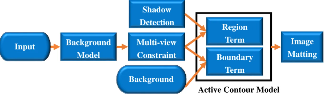
Chapter 3 Proposed Algorithm

The goal of our work is to accurately extract foreground regions with smooth boundary. After we extract the foreground regions, we can combine computer-generated environment or interested background with the foreground regions in a seamless manner. Our foreground detection method requires only to distinct foreground from background which is obtained using the standard Mixture of Gaussian background modeling technique. Combining foreground regions with multi-view spatial constraints would allow us to automatically and simultaneously segment foreground and background regions in a multiple camera system. We further overcome the drawbacks of the background modeling method in outdoor scenes when illumination changes a lot. We use a nonlinear tone mapping, termed Matching by Tone Mapping [19], to evaluate the distance between suspected foreground and background pixels.

We propose to apply continuous-domain convex active contour with the distance between suspected foreground and background pixels to generate the initial foreground. The convex active contour is then applied in the second step to optimize the contour. After that, we exploit the image matting model to obtain the final foreground segmentation. Unlike the traditional way that calculates the matting laplacain in RGB color space, we extend the element of the matting laplacian to a higher dimension to get more accurate foreground. In Figure 3-1, we show the flow chat of our system. In this chapter, the details of our method will be introduced.

Figure 3-1 Flowchart of our algorithm

Active Contour Model

Image Matting Multi-view Constraint Background Model Shadow Detection Region Term Boundary Term Input Image Background Image

14

3.1 Background Modeling

Background modeling and foreground detection is a way to detect foreground objects in images acquired by static cameras. The importance of such methods has given rise the birth of approaches. According to [20], one of the most effective and popular method is the one proposed by Stauffer and Grimson [21] which models the appearance of each image pixel as a mixture of Gaussians. These gaussian functions are combined to provide a multimodal density function. They can be employed to model the color of an object in order to perform tasks such as real-time color-based tracking and segmentation. These tasks may be made more robust by generating a mixture model corresponding to background colors in addition to the foreground model, and by employing Bayes' theorem to perform pixel classification.Mixture models are a semi-parametric alternative to non-parametric histograms and can provide greater flexibility and precision in modelling the underlying statistics of the sample data. They are able to smooth over gaps resulting from sparse sample data and provide tighter constraints in assigning object membership to color-space regions. Such precision is necessary to obtain the best results possible from color-based pixel classification for qualitative segmentation requirements. Given a sequence of images, the background model is estimated from a training time. Each pixel is

modeled as a 𝐾 component Gaussian Mixture Model (GMM) given by

𝑃𝑋|𝑘(𝑋|𝑘, 𝜃𝑘) = 1 (2𝜋)𝑛2_|𝛴𝑘|12𝑒

−1₂(𝑋−𝜇𝑘)𝑇𝛴𝑘−1(𝑋−𝜇𝑘)_{, and (3-1)}

𝑃𝑋(𝑋|𝛩) = ∑𝑘=𝐾𝑘=1𝑝(𝑘)𝑃𝑋|𝑘(𝑋|𝑘, 𝜃𝑘), (3-2)

where the mixing parameter 𝑝(𝑘) corresponds to the prior probability that the pixel 𝑋 is generated by component k, and the sum of 𝑝(𝑘) equals to one. Each mixture component is a Gaussian with the mean 𝜇 and the covariance matrix 𝛴. Once a model is generated, conditional probabilities can be computed.

15

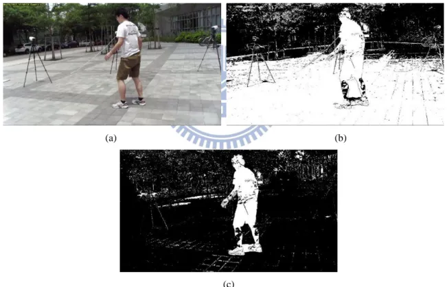
After the foreground detection step, an initial mask is generated. However, the existence of camera noise and irregular background object motion and the illumination variations in outdoor scene may degrade the performance of foreground detection. In figure 3-2, we show an example of initial foreground mask got from GMM background modeling by directly subtracting the background image. Here, the background image is got form median filter, which assumes the background is static. By filtering a sequence of images via median filter, we can filter out moving objects and remain the static background image. We can see in Figure 3-2 (b) that the result is full of background noise because of the cloudy weather. In contrast, the GMM background modeling can handle this situation in a more robust way but may still have some noise due to severe background variations. We will eliminate the noise in the next section.

(a) (b)

(c)

Figure 3-2 Comparison the foreground detection. (a) Original image (b) Foreground detection from directly subtraction (c) Foreground detection from GMM background modeling

3.2 Spatial Consistency for multi-view

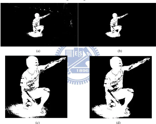
` A simple way to remove the noise regions after background modeling is to use morphology operations. The “close” operation or the connected component analysis is effective for

16

eliminating the background noise. However, the size of the structure element is important. To remove large noise region, a larger structure element should be used. However, the use of a large structuring element may cause the loss of the foreground information and degrade the precision of object boundary. Figure 3-3 shows the foreground degradation example by using a morphological process. As shown in Figure 3-3(b), though the noise is totally eliminated by the morphology filter, the foreground regions in the armpit and the belly is also filtered out due to the narrow connections between the foreground regions.

(a) (b)

(c) (d)

Figure 3-3 Traditional way to eliminate background noise by using morphology operator. (a) GMM background modeling of Figure 2-3(a). (b) Denoise by morphology operator result of (a). (c)Zoom in of (a). (d)Zoom in of (b).

In this section, we propose a method which combines multi-view constraints to eliminate the background noise while remaining the foreground regions mostly. By assuming the shadow areas locate on the ground, we can use the homography geometry constraint to remove shadows and to extract more accurate foreground regions. The homography geometry constraint will be

17 discuss in section 3-5.

In fact, foreground regions should have the property that there exists a 3D region that projects onto several camera views. This is known as spatial coherence or called silhouette consistency constraint [22]. A set of silhouettes defines a visual hull [23], which is the interaction of the backprojection of silhouettes into the 3D space. Placing a cube in 3D region and checking what is outside the object silhouette, anything outside is carved away. The silhouette calibration ratio define in [22] is a purely geometric measure that tells whether a pixel belongs to a foreground region according to the other foreground regions from different viewpoints. Similar to this concept, we adopt a silhouette consistency constraint to remove these noisy regions. In this constraint, we assume the foreground object shall appear in all image views. We build up the fundamental matrix between the reference image and other images. Fundamental matrix is a 3 × 3 matrix, which relates corresponding points in a pair of image views. In epipolar geometry, with XL and XR, representing corresponding points in an image

pair, F·XL describes a line (an epipolar line) on which the corresponding point XR on the other

image must lie. That means, all pairs of corresponding points hold x′Fx = 0. An epipolar geometry is shown in Figure 3-4 (a).

18

Figure 3-4 Epipolar Geometry (a) Image pair with fundamental matrix related to a point mapping to other image is a line (b) input image (view 1) (c) input image (view 2)

As shown in Figure 3-4 (b)(c), we can see the points along the line corresponding to the same line to the other image. Using this epipolar constraint, even we have elliminated some points on the line, there still are other points which can map to the same line in the other image. Hence, after camera calibration, we first eliminate most noise on different camera views by projecting all candidate foreground regions into the same reference camera view and only keep the intersection region. Figure 3-5 illustrates this concept. We can effectively remove most background noise and the foreground region is remained completely. Figure 3-6 shows another case of multi-view constraint to eliminate the background. The difference between Figure 3-5 and Figure 3-6 is that the camera positions in Figure 3-5 are greatly rotated and placed far away between each other

.

(a) (b) (c)

19

Figure 3-5 Multi-view constraint for denoising (Take view 4 for reference view). (a) Camera postion. (b) View 1 (c) View 2 (d) View 3 (e) View 4 (f) View 5 (g) View 6 (h) GMM modeling of (b). (i) GMM modeling of (c). (j) GMM modeling of (d). (k) Denoise of (h). (l) Denoise of (i). (m) Denoise of (j). (n) Viewing-ray interaction. (o) Output of multi-view constraint.

Camera 1

Camera 3

Camera 4(Reference view)

Camera

5

_Camera

6

Camera 2

(b) (a) (b) (c) (d) (e) (f) (g) (h) (i) (j) (k) (l) (m) (n) (o)

20

Figure 3-6 Multi-view constraint for denoising (Take view 3 for reference view). (a) Camera postion. (b) View 1 (c) View 2 (d) View 3 (e) View 4 (f) View 5 (g) View 6 (h) GMM modeling of (b). (i) GMM modeling of (e). (j) GMM modeling of (f). (k) Denoise of (h). (l) Denoise of (i). (m) Denoise of (j). (n) Viewing-ray interaction. (o) Output of multi-view constraint.

(b) (a) (b) (c) (d) (e) (f) (g) (h) (i) (j) (k) (l) (m) (n) (o)

21

Using epipolar geometry, we are no longer restricted to short base-line multiple-camera systems, but can handle wide base-line multiple-camera system. As shown in Figure 3-5 and Figure 3-6, the more far away the cameras are placed, the better the denoising result is. However, there may still remain some noise because of the dramatic color variation in the outdoor scene. Such noise can be suppressed by adding more image views. Considering the number of viewpoints are generally fixed in practice, we will propose more processes to eliminate this noise in the next section.

3.3 Convex Active Contour Model

The scheme described in the previous section discriminates background from foreground regions in a multi-view system. However, it still remains some noisy regions which are caused by sudden sunlight change, cloudy weather or irregular background variation. In this section, we use the convex active contour model described in Equation 2-1 to generate the initial foreground segmentation. This model can find the global minimum solution and can be used for automatic image segmentation. As expressed in Equation 2-1, the active contour model consist of two terms: a regional term and a boundary term. Next we will discuss how to design these two terms to get the initial foreground segmentation.

3.3.1

Region Term Formulation

After GMM background modeling, some background noise remains. We assume that no matter in a sunny day or a cloudy day the structural content (namely, textures and edges) in those noisy regions does not change, but only their illumination changes.

To overcome background noise, we assume there is a nonlinear tone mapping between the suspected pixels and background pixels; namely, the spatial neighboring of a suspected pixel in the current frame is a result of a nonlinear tone mapping of the corresponding spatial location in the background image. Unlike linear tone mapping, which can deal with the Normalized

22

Cross Correlation (NCC) metric, the nonlinear mapping does not restrict the transformation within the background noise of the image. This nonlinear mapping can thus model any tone mapping (including non-monotonic mappings). Hence, we use Matching by tone Mapping (MTM) distance metric to measure the difference between suspected patch and background patch, which is proposed by Hel Or et al. [19] as shown in Figure 3-7

(a) (b)

Figure 3-7 MTM distance measure between input image and background image patch by patch. (a) background image (b) input image

MTM distance measure can distinguish between the suspected pixels and background pixels. This distance metric can be used to distinguish foreground objects from background noise which only have non-linear illumination change. The MTM metric compensates for the nonlinear mapping which exists in the suspected pixels and results in a small distance value. If foreground pixels greatly differ from the background pixels, the MTM measure produces a large distance value. The MTM measure is robust for different scenes. The MTM measure can also handle low-quality images and complex lighting conditions. The MTM measure defined as follows: D(p, w) min M { ||𝑀(𝑝) − 𝑤||2 𝑚 ∙ 𝑣𝑎𝑟(𝑤) }, (3-3)

where pϵRm and wϵRm are the two patches to be compared. The function M: R → R is a tone mapping function. MTM distance measure is tone-scale invariant because the denominator is a normalization factor. That is, D(p,w)=D(p,αw) for any α. This can avoid trivial solution if

23

In a recent study [19], Hel Or et al. [19] proposed an efficient method to compute MTM using piecewise-constant mapping approximation. which has the closed form follows:

D(p, w) = 1 m ∙ var(w)[||w|| 2 − ∑ 1 |𝑃𝑗_|(𝑝𝑗∙ 𝑤) 2 𝑗 ], (3-4)

where the range of p is divided into k bins and k binary “slices” of p are produced. Denoting the jth _{slice by p}j_{, each of which representing the pixels belonging to this respective bin. The}

details are described in [19]. Based on its definition, MTM can distinct two patches by producing a “distance map”, where small values relate to noisy regions whereas high values indicate a different content, namely, foreground pixels regardless of brightness and contrast changes.

The original MTM distance measures the input image and background patch by patch. Since the patch in input image may contain both foreground regions and background regions, the distance measurement may not be able to separate them. The proposed method use MTM measurement to measure the distance value only in the multi-view constrained GMM mask instead of searching the entire images. Note that we use a small structuring element to remove small regions before MTM distance measurement. Figure 3-8 shows the result with MTM distance measurement. As shown in Figure 3-8 (f), the shadow area and the noisy region is highly related to the background image through a non-linear tone mapping. Hence, the MTM distance measure is small. By using MTM distance measure, we can separate foreground regions from background rergions, including the shadow area. In order to make sure the region is consistent in foreground region, we typically use a large window size in MTM distance measurement. Though the noisy region may be indistinct because the window around foreground may also contain foreground region as shown in Figure 3-8 (e), we can use the boundary term in the active contour model to optimize the foreground contour. This can eliminate the noise around foreground region. Moreover, the background reference image is

24

obtained by applying the median filter over a sequence of background images, in which the background is static. Figure 3-9 shows more examples of MTM distance measurement.

(a) (b)

(c) (d)

(e) (f)

Figure 3-8 The MTM distance measure map. (a) Original image (b) Search entire image with window size 300 (c) Search entire image with window size 200 (d) GMM mask through multi-view constraint and simple morphology operator (e) MTM measure of (d) with window size 300. (f) MTM measure of (d) with window size 200.

We incorporate this regional information derived from MTM into the region term of the convex active contour model as

h_r(𝑥) = 1 − 𝐷(𝑝, 𝑤), (3-5)

where x denotes an image pixel and p and w denote the image patches around x on the background reference image and the current image. This definition of hr ensures that the active

25

contour evolves toward the one complying with the MTM measure. For instance, for a pixel, if D(p,w) is low and hr becomes larger, u(x) tends to increase during the energy minimization in

(1) in order to get contour evolution. This leads to a u(x) value beneath the threshold T and the pixel is classified as background.

(a) (b)

(c) (d)

(e) (f)

Figure 3-9 The MTM distance map. (a) MTM measure of Figure 3-5(o). (b) MTM measure of Figure 3-6(o). (c) Input image. (d) GMM mask through multi-view constraint. (e) MTM measure of (d) with window size 300. (f) MTM measure of (d) with window size 300.

3.3.2

Boundary Term Formulation

26

Equation (2-1), the boundary term ∫ 𝑔_{Ω 𝑏}|∇𝑢|𝑑𝑥 is essentially a weighted variation of function 𝑢, where the g_b plays an important role.The definition of g_b in Equation (2-3) encourages the segmentation along the curves where the value of edge detection function is small so the variation of the function u is minimal. However, there may exist lots of noisy edge since the background is a non-uniform outdoor scene. Hence, in this thesis, we propose a simple method to reduce noisy edge shown in outdoor background. The input images and background image are filtered by a gradient filter. After that, we take the difference between them. That is, we define the gb value at pixel x as:

gb(𝒙) = |𝑓(𝒙)| − |𝑟(𝒙)|, (3-6)

where  denotes the gradient operation and f(x) and r(x) represent the pixel value at the input image and the background reference image, respectively. Figure 3-10 compares the result with and without incorporating the edge detection of the background image. It can be seen from Figure 3-10 that the inclusion of |𝑟(𝒙)| enhances the conventional edge detection result and leads to a more accurate boundary contour to reduce the effect of noisy edge. Note the edge detection function returns a value between 0 to 1; a small value of g_b corresponds to a possible edge.

Based on the MTM distance map in the region term and the refinement gb(x) image in

Figure 3-10, we obtain the u(x) image by solving Equations (3-1) based on the convex active contour method.

27

Figure 3-10 Comparison of the results with and without |𝑟(𝒙)| in edge detection function. (a)Result using |f(𝐱)|. (b) Result using |𝑟(𝒙)|. (c) Result using Equation (3-6).

The initial foreground segmentation results are shown in Figure 3-11, which can be seen that the foreground object has been automatically identified with reasonable precision, even with a challenging outdoor environment.

(a) (b)

Figure 3-11 Result of active contour output. (a) Active contour output of Figure 3-5 (o). (a) Active contour output of Figure 3-6 (o).

Combining the convex active model leads to more accurate boundary contours. (a)

(b)

28

Segmentation result will be further fine-tuned based on the image matting method.

3.4 Image Matting Model

The last stage of our proposed method is to apply an image matting model to get the final segmentation result. In the literature, supervised image matting is based on the similarity of colors between the unknown pixels and some samples of foreground pixels and background pixels. In the image matting model, the color of a pixel can be expressed as a linear combination of the corresponding foreground and background colors; that is,

I_i = 𝛼_𝑖𝐹_𝑖+ (1 − 𝛼_𝑖)𝐵_𝑖. (3-7)

Figure 3-12 Image matting model

Equation (3-7) can be pictured as illustrated in Figure 3-12, where we need to compute the alpha matte based on the matting model. As expected, the more alpha value is, the more likely the pixel belongs to the foreground object. For supervised image matting in [6], Levin et al. assume the alpha matte may be represented locally as a linear combination of the image color channels. They introduce the use of matting Laplacian (ML) to compute the alpha matte without explicitly estimating the foreground and background colors in Equation (3-7). ML can be expressed as ∑ (𝛿_𝑖𝑗− 1 |𝑊𝑘|(1 + (𝐼𝑖− 𝜇𝑘) (Σ𝑘+ 𝜖 |𝑤𝑘|𝐼3) −1 (𝐼_𝑗− 𝜇_𝑘)) , 𝑘|(𝑖,𝑗)𝜖𝑤𝑘 (3-8)

where Ii and Ij are the color values of the input image, 𝜇_𝑘 is a 3 × 1 mean color vectors in

29

drawback of ML is that it may have incorrect propagation across foreground regions because of the use of low quality outdoor surveillance cameras and the severe color variations in outdoor scenes.

The first thing in supervised image matting is to label two types of strokes as foreground pixels and background pixels. However, even though this ML approach can achieve quite impressive performance for foreground object extraction, it has difficulty in handling outdoor scenes under dramatic brightness variations or color variations. In Figure 3(b) and Figure 2-4(b), we show the manually selected scribbles for the image in Figure 2-3(a) and 2-4(a). Based on the scribbles, the corresponding matting result generated by the ML method is shown in Figure 2-3(c) and Figure 2-4(c).

Instead of using manually selected scribbles, our system can automatically generate the required trip-map for the ML method. This tri-map is obtained by the initial foreground segmentation got from the active contour model. As expressed in Equation (2-2), the tri-map is obtained by taking a threshold over the u(x) image. Above the threshold T1, we define the region

as a foreground region; otherwise, it should be a background region if the value of u(x) is beneath the threshold T2. After that, a morphological erosion operation is applied over both the

foreground regions and the background regions to obtain the unknown regions, as shown in Figure 3-13.

Figure 3-13 Automatically generated tri-map based on active contour model.

More specifically, for each pixel in unknown regions, the matting algorithm is the process of extracting a foreground object from an image. Based on this tri-map and the color similarity

30

between the unknown pixel and the samples foreground and background samples, the alpha value of the unknown pixel is estimated. We can obtain a much better matting result as shown in Figure 3-14(a).

To further improve the matting result, we add in more information in the computation of the affinity values. In the original ML method, they only consider the RGB color values in the computation of the affinity value to reduce foreground region propagation across background and to produce a smooth and accurate boundary contour. Instead of the original ML which only considers the RGB color space to separate foreground regions from background regions, here, we include extra image features: the absolute value of the difference image between the input image and the background reference image. The extra features can help in generating more accurate boundaries between the foreground objects and the background. In Figure 3-14, we further show the comparison between the supervised image matting method and the proposed automatic method in the embedding of the foreground object into the virtual scene. It can be seen that, except the shadow part, the proposed system can generate more accurate and natural result. The removal of shadows will be the next goal of our system.

(a) (b)

31

3.5 Shadow Removal

The proposed method can extract foreground objects with reasonable precision, but the shadow is also extracted. In some applications, the synthesized image may look absurb and unnatural because of the shadow, as shown in Figure 3-15. We will discuss and remove the shadow in this section.

Figure 3-15 Shadow effect in synthesized image caused contrived result.

Shadow in many applications, such as object tracking, video surveillance, may appear as foreground objects. The inability to distinguish between foreground objects and shadows can cause some problems, such as weird synthesized image in virtual studio and failure of identification. Hence, shadow detection and removal is an important task.

To remove shadows, we assume the shadow areas are on the ground. Consider a scene containing a reference plane being viewed by a set of wide-baseline stationary cameras. The background models in each view are available. Any scene point lying inside the foreground zone in the scene will be projected to a foreground pixel in every view. Instead of using the fundamental matrix, we reduce the dimension in the fundamental matrix. We only concentrate our attention on the ground plane, which is called homography constraint, as shown in Figure 3-16. After reducing the dimension in fundamental matrix, we can map a point in one view to

32

a point in another view. The homography matrix warps a pixel from image to another on a reference scene planeπ.

Figure 3-16 Homography constraint show that a pixel in one view are warping to another view by a reference plane (ground).

Let Ф1,Ф2 , … ,Фn be the images of the scene obtained from n calibrated cameras. Hiπ𝑟 is homography of the reference plane π between the reference plane and any other view i. Using homography matrix H_iπ𝑟, pixel as suspected foreground pixels in all the other images are warped to the reference image. The warping result are thresholded to get categorized as a shadow area, where can write this term as:

δ(x) = {1

₀

,

𝑛>|𝐶|2

𝑜𝑡ℎ𝑒𝑟𝑤𝑖𝑠𝑒

(3-8)

In Equation (3-8), |C| is the number of cameras. Typically we set the threshold to be a half of the camera number. The results of shadow detection are shown in Figure 3-17.

33

(a) (b)

Figure 3-17 Shadow detection. (a) Shadow on the ground. (b) MTM distance measure.

In Figure 3-17(a), the shadow areas which assume to be on the ground are marked in black. Though the shadow areas can be well detected, some foreground objects like the shoes near the ground may also get detected. If we directly remove the area on the ground, the result will be poor because of the foreground region near the ground. By using the MTM distance measure mentioned before, we can distinguish the exact foreground regions from the shadow regions,

34

as shown in Figure 3-17 (b). Note that we use a smaller window to measure the ground (marked as black) region patch by patch to get a more accurate separation. By combining the active contour model and the image matting method, we can get the final segmentation result as shown in Figure 3-18.

Figure 3-18 Shadow removed result.

In fact, the result of Figure 3-18 still have some shadows left around the outer shadow area because the shadow area detected by homography constraint is smaller than the GMM background modeling This leads to imperfect result. The problem can be solved by applying multi-view constraint mentioned in Section 3-2 to further eliminate the shadow area. We can first use the homography constraint to detect the shadow area and then apply MTM distance measure to separate foreground from the ground. After that, we project all detected shadow regions to the reference view and the interaction region remains as the final result. The use of multi-v0iew constraint to remove shadow area is demonstrated in Figure 3-19.

35

Figure 3-19 Multi-view constraint with shadow detection. (a) Original image. (b) GMM modeling of (a). (c) Multi-view constraint with shadow removed.

(a)

(b)

36

Chapter 4

Experimental Results

In Figure 4-1, we show more simulation results on the other camera views. It can be seen that the foreground object can be effectively extracted in a quite accurate form, in spite of the complicated background environments. Note in Figure 4-1, the homography constraint to remove shadow is not included yet. It can be seen that, except the shadow part, the proposed system can generate accurate and natural results.

Figure 4-1 More results on other camera views. (a) Original image. (b) Multi-view constraint. (c) Result of convex active contour model. (d) Result of modified image matting method.

(a)

(b)

(c)

37

In Figure 4-2, we show the comparison between the supervised image matting method and the proposed automatic method in the embedding of the foreground object in a virtual scene. It can be seen that, with the homography constraint to remove shadows, the final foreground region has more accurate and smoother boundary.

Figure4-2 Comparison between the supervised image matting method and the proposed automatic method (a) Manually selected scribbles. (b) Synthesized image based on (a) and the original ML method. (c) Automatically generated tri-map. (d) Synthesized image based on (c) and the modified ML method.

In Figure 4-3, we further show the comparison between the original image matting

methods which only considers RGB color values, and the modified image matting method. As

expressed before, the boundary of the foreground in Figure 4-2 (a) is mixed with the background because of the dramatic color variations and the color similarity between foreground regions and background regions. The modified ML method has more precise boundary around the foreground object.

38

(a) (b)

Figure 4-3 Comparison between original ML and modified method of Figure 2-4(a). (a) Original ML method. (b) Modified Ml method.

In Figure 4-4 to Figure 4-6, we show the comparison of the active contour model, the image matting model methods which only considers RGB color values, and the modified image matting method. The active contour model still has some broken foreground regions though the foreground objects is accurately separated from the background image. Based on the active contour model, the image matting model can accurately find the broken foreground. The modified matting laplacian can separate foreground object from background precisely. Note that even the foreground object is dressed in different colors, the proposed method can still separate the foreground object from the background accurately.

39

Figure 4-4 Compariosn of active contour model and image matting model. (a) Input image. (b) Active contour model. (c) Original image matting. (d) Modified image matting.

(a)

(b)

(c)

40

Figure 4-5 Compariosn of active contour model and image matting model. (a) Input image. (b) Active contour model. (c) Original image matting. (d) Modified image matting.

(a)

(b)

(c)

41

Figure 4-6 Compariosn of active contour model and image matting model. (a) Input image. (b) Active contour model. (c) Original image matting. (d) Modified image matting.

(a)

(b)

(c)

42

In Figure 4-7, we show more embedding examples of the foreground object into virtual scenes. The proposed method can accurately separate foreground from background in outdoor scenes. (a) (b) (c) (d) (e) (f)

43

Figure 4-7 More result of the foreground object into the virtual scene. (a)(d)(g)(j) Input image. (b)(e)(h)(k) Foreground extraction. (c)(f)(i)(l) Synthesized image.

In our experimental result to generate synthesized image, wesmooth the object boundary in order to generate more natural result in the embedding of the foreground object into computer generated environments. To smooth the boundary we take the alpha value to be between 0.1 to 0.9.

(g) (h)

(i) (j) (k) (l)

44

Chapter 5 Conclusion

In this thesis, we present a novel method to automatically separate foreground objects from the background in an outdoor scene. To suppress the noise generated in the background subtraction process, we include a multi-view constraint to combine information from different camera views. We further build a convex active contour model to obtain more reliable object boundaries. Finally, we propose a modified image matting method to get fine-tuned segmentation results. Experimental results demonstrate that the proposed method can outperform existing methods for outdoor-scene foreground/background separation without the inclusion of user guidance.

45

References

[1] S.-y. Chien, S.-y. Ma, and L.-g. Chen, "Efficient moving object segmentation algorithm using background registration technique," IEEE Transactions on Circuits and Systems for Video Technology, vol. 12, pp. 577-586, 2002.

[2] C. Rother, V. Kolmogorov, and A. Blake, "GrabCut": interactive foreground extraction using iterated graph cuts," ACM Transactions on Graphics - TOG , vol. 23, pp. 309-314, 2004.

[3] L. Grady, "Random Walks for Image Segmentation," IEEE Transactions on Pattern Analysis and Machine Intelligence, vol. 28, pp. 1768-1783, 2006.

[4] X. Bai and G. Sapiro, "A Geodesic Framework for Fast Interactive Image and Video Segmentation and Matting," the International Conference on Computer Vision, 2007. [5] A. Criminisi, T. Sharp, and A. Blake, "GeoS: Geodesic Image Segmentation," in

Computer Vision – European Conference on Computer Vision, pp. 99-112, 2008. [6] A. Levin, D. Lischinski, and Y. Weiss, "A Closed-Form Solution to Natural Image

Matting," IEEE Transactions on Pattern Analysis and Machine Intelligence, vol. 30, pp. 228-242, 2008.

[7] M. Piccardi, "Background subtraction techniques: a review," IEEE International Conference on Systems, Man, and Cybernetics, vol. 4, pp. 3099-3104, 2004.

[8] A. M. Elgammal, D. Harwood, and L. S. Davis, "Non-parametric Model for Background Subtraction," European Conference on Computer Vision, pp. 751-767, 2000.

[9] D. Culibrk, O. Marques, D. Socek, H. Kalva, and B. Furht, "Neural Network Approach to Background Modeling for Video Object Segmentation," IEEE Transactions on Neural Networks, vol. 18, pp. 1614-1627, 2007.

[10] M. Kass, A. Witkin, and D. Terzopoulos, "Snakes: Active contour models," International Journal of Computer Vision, vol. 1, pp. 321-331, 1988/01/01 1988. [11] V. Caselles, R. Kimmel, and G. Sapiro, "Geodesic Active Contours," International

Conference on Computer Vision , pp. 694-699, 1995.

[12] T. F. Chan and L. A. Vese, "Active contours without edges," IEEE Transactions on Image Processing, vol. 10, pp. 266-277, 2001.

[13] X. Bresson, S. Esedoglu, P. Vandergheynst, J.-P. Thiran, and S. Osher, "Fast Global Minimization of the Active Contour/Snake Model," Journal of Mathematical Imaging and Vision, vol. 28, no. 2, pp. 151-167, 2007.

[14] T. Goldstein, X. Bresson, and S. Osher, "Geometric Applications of the Split Bregman Method: Segmentation and Surface Reconstruction," Journal of Scientific Computing, vol. 45, no. 1-3, pp. 272-293, 2010.

[15] V. Kolmogorov, A. Criminisi, A. Blake, G. Cross, and C. Rother, "Probabilistic Fusion of Stereo with Color and Contrast for Bilayer Segmentation," IEEE Transactions on

46

Pattern Analysis and Machine Intelligence, vol. 28, pp. 1480-1492, 2006.

[16] G. Zeng, "SILHOUETTE EXTRACTION FROM MULTIPLE IMAGES OF AN UNKNOWN BACKGROUND," Asian Conference on Computer Vision, 2004.

[17] M. Sormann, C. Zach, and K. F. Karner, "Graph Cut Based Multiple View Segmentation for 3D Reconstruction," 3D Data Processing Visualization and Transmission, pp. 1085-1092, 2006.

[18] W. Lee, W. Woo, and E. Boyer, "Silhouette Segmentation in Multiple Views," IEEE Transactions on Pattern Analysis and Machine Intelligence, vol. 33, pp. 1429-1441, 2011.

[19] Y. Hel-Or, H. Hel-Or, and E. David, "Fast template matching in non-linear tone-mapped images," International Conference on Computer Vision, pp. 1355-1362, 2011.

[20] T. Bouwmans, F. E. Baf, and B. Vachon, Background Modeling using Mixture of Gaussians for Foreground Detection - A Survey, 2008.

[21] C. Stauffer and W. E. L. Grimson, "Adaptive Background Mixture Models for Real-Time Tracking," Computer Vision and Pattern Recognition, vol. 2, pp. 2246-2252, 1999. [22] E. Boyer, "On Using Silhouettes for Camera Calibration," Asian Conference on

Computer Vision, pp. 1-10, 2006.

[23] A. Laurentini, "The Visual Hull Concept for Silhouette-Based Image Understanding," IEEE Transactions on Pattern Analysis and Machine Intelligence, vol. 16, pp. 150-162, 1994.