在數位訊號處理器中利用記憶位址產生器之間接位址模式作陣列索引計算最佳化

全文

(1)國立交通大學資訊工程系碩士論文. 在數位訊號處理器中利用記憶位址產生器之間接位址模式作陣列索引計算最佳化. Optimizing Array Index Computation with Indirect Addressing of the AGU in a DSP. 研究生：陳俊一指導教授：單智君博士. 中華民國九十三年八月 i.

(2) 在數位訊號處理器中利用記憶位址產生器之間接位址模式作陣列索引計算最佳化. Optimizing Array Index Computation with Indirect Addressing of the AGU in a DSP 研究生：陳俊一. Student：Chun-Yi Chen. 指導教授：單智君博士. Advisor：Dr. Jean, Jyh-Juin Shann. 國立交通大學資訊工程學系碩士論文 A Thesis Submitted to Department of Computer Science and Information Engineering College of Electrical Engineering and Computer Science National Chiao Tung University in Partial Fulfillment of the Requirements for the Degree of Master In Computer Science and Information Engineering June 2004 Hsinchu, Taiwan, Republic of China. 中華民國九十三年八月. ii.

(3) 在數位訊號處理器中利用記憶位址產生器之間接位址模式作陣列索引計算最佳化. 學生：陳俊一. 指導教授：單智君博士. 國立交通大學資訊工程學系碩士班. 摘要由於大多數的數位訊號處理之相關應用程式（例如影像處理、音訊處理）大量存取記憶體內的陣列資料，使得計算這些陣列位址所造成的負擔對於程式執行效能與程式碼大小有很大的影響。有些數位訊號處理器配有記憶位址產生器，只需少量的位元數編碼在指令中就可以快速計算位址，不但減少程式碼的大小，也可加速程式執行速度，在本論文中，我們提供兩個方法來解決如何將迴圈內陣列參考分配給固定數量之位址暫存器與修改暫存器，使得迴圈內計算位址之指令數最少的問題。其中一種為刪除法，此方法針對較小的問題可以找到最佳解。另一個方法為基因演算法，對於那些較大的問題，透過有效率的步驟，可以找到合適的解。與過去的研究相較之下，實驗結果顯示我們的方法確實有較好的效果。. iii.

(4) Optimizing Array Index Computation with Indirect Addressing of the AGU in a DSP Student：Chun-Yi Chen. Advisor：Jean, J.J Shann. Institute of Computer Science and Information Engineering National Chiao-Tung University. Abstract Since most DSP applications (video/audio processing) access a large amount of array elements stored in memory, the address computation overhead of array elements has great impact on performance and code size. Some DSPs are equipped with dedicated address generation units (AGUs). The AGU enables fast address computation with few bits encoded into an instruction, resulting in code size reduction as well as performance improvement of programs. In this thesis, we provide two approaches to solve the problem of clustering array references in loops to fixed number of address registers and modify registers so that the number of instructions needed for address computations in loops is minimized. One is pruning method which can solve small-size problems to obtain optimal solutions. The other is genetic algorithm which can solve large problems to obtain reasonable solutions in an efficient way. Experimental results show that our approaches are indeed more effective compared to previous work.. iv.

(5) 誌謝首先感謝我的指導老師單智君教授，在老師的諄諄教誨、辛勤指導與勉勵下，我得以順利完成此論文，並且順利通過畢業口試。同時感謝我的口試委員鍾崇斌教授以及謝萬雲教授，由於他們的指導與建議，讓這篇論文更加完整和確實。. 此外，感謝實驗室的學長—鄭哲聖學長、喬偉豪學長和林漢君學長，每次都不厭其煩地跟我討論許多問題，給予我莫大的幫助。也感謝實驗室全體學長姐、同學以及學弟們，真的很高興可以認識你們大家。因為你們，讓我的研究生活充滿了歡樂。. 最後感謝我的家人，謝謝你們在背後全心全意地支持我，讓我在這研究的路上走得更順利，進而能無後顧之憂的學習，讓我追求自己的理想。. 謹向所有支持我、勉勵我的師長與親友，奉上最誠摯的祝福，謝謝你們。. 陳俊一 2004. 8. 15. v.

(6) Table of contents 摘要............................................................................................................. iii Abstract ........................................................................................................iv 誌謝...............................................................................................................v Table of contents ..........................................................................................vi List of Figures........................................................................................... viii List of Tables.................................................................................................x Chapter 1. Introduction .............................................................................1. 1.1. Research Motivations.................................................................................. 2. 1.2. Research Objective and Proposed Approaches........................................... 3. 1.3. Organization of This Thesis ........................................................................ 3. Chapter 2. Backgrounds and Related Work ..............................................4. 2.1. The Address Generation Unit in DSP ......................................................... 4. 2.2. Genetic Algorithms ..................................................................................... 5 2.2.1. Selection Operators.............................................................................. 6. 2.2.2. Crossover Operators ............................................................................ 7. 2.2.3. Mutation Operators .............................................................................. 8. 2.2.4. Termination Methods ........................................................................... 9. 2.3. Previous Works ......................................................................................... 10 2.3.1. Local Array Reference Allocation (LARA)....................................... 10. 2.3.2. Global Array Reference Allocation (GARA)..................................... 15. 2.3.3. Summary of Address Code Optimization with AGU......................... 16. Chapter 3. Proposed Methods .................................................................18. 3.1. Observation ............................................................................................... 18. 3.2. Problem Description ................................................................................. 20 vi.

(7) 3.3. Problem Transformation ........................................................................... 20. 3.4. Approach 1: Brute Force with Pruning ..................................................... 23 3.4.1. 3.5. Time Complexity ............................................................................... 28. Approach 2: Genetic Algorithm (GA) ...................................................... 29 3.5.1. Overview of GA................................................................................. 29. 3.5.2. Chromosomal Representation............................................................ 30. 3.5.3. Population Initialization..................................................................... 31. 3.5.4. Crossover and Mutation Operation.................................................... 32. 3.5.5. Evaluation Function........................................................................... 34. 3.5.6. Parameters.......................................................................................... 36. 3.5.7. Time complexity ................................................................................ 36. Chapter 4. Simulation and Analysis........................................................37. 4.1. Benchmark Suite....................................................................................... 37. 4.2. Experimental Results ................................................................................ 38 4.2.1. Chapter 5. Summary of Experimental Results .................................................... 43. Conclusion and Future Works ...............................................44. References...................................................................................................45. vii.

(8) List of Figures Figure 1-1 Execution time overhead and memory overhead .................................. 1 Figure 2-1 AGU Block Diagram............................................................................. 4 Figure 2-2 Top-level description of a genetic algorithm......................................... 6 Figure 2-3 Array references and the distance graph ............................................. 11 Figure 2-4 Extended distance graph ..................................................................... 12 Figure 2-5 CFG fragment after Ø-insertion and reference analysis ..................... 16 Figure 3-1 Modified distance graph...................................................................... 21 Figure 3-2 Modified extended distance graph (MEDG)....................................... 22 Figure 3-3 (a) A source program (b) MEDG ........................................................ 23 Figure 3-4 Two cases when considering node 2 ................................................... 24 Figure 3-5 Two cases when considering node 3 of case 1 in Figure 3-4 .............. 24 Figure 3-6 Two cases when considering node 4 of case 1 in Figure 3-5 .............. 25 Figure 3-7 All combination of above example ..................................................... 26 Figure 3-8 Flow chart of our GA .......................................................................... 30 Figure 3-9 (a) a source program (b) MEDG (c) chromosome representation ...... 31 Figure 3-10 An example of initial population....................................................... 32 Figure 3-11 One-point crossover operation .......................................................... 33 Figure 3-12 Bit mutation operation....................................................................... 33 Figure 3-13 An example of calculating a chromosome of evaluation function.... 35 Figure 4-1 Addressing costs of 1 AR and l MRs for small programs ................... 39 Figure 4-2 Addressing costs of 2 ARs and l MRs for small programs ................. 40 Figure 4-3 Addressing costs of 3 ARs and l MRs for small programs ................. 40 Figure 4-4 Addressing costs of 4 ARs and l MRs for small programs ................. 40 Figure 4-5 Addressing costs of 1 ARs and l MRs for all programs ...................... 41 viii.

(9) Figure 4-6 Addressing costs of 2 ARs and l MRs for all programs ...................... 41 Figure 4-7 Addressing costs of 3 ARs and l MRs for all programs ...................... 42 Figure 4-8 Addressing costs of 4 ARs and l MRs for all programs ...................... 42. ix.

(10) List of Tables Table 2-1 Comparison of related work and our problem ...................................... 17 Table 4-1 Stencil Micro-Benchmarks Suite .......................................................... 38 Table 4-2 Addressing costs reduction for small programs.................................... 41 Table 4-3 Addressing costs reduction for all programs......................................... 42. x.

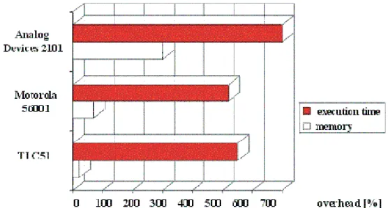
(11) Chapter 1. Introduction. More and more DSP system designs are based on software running on programmable processors rather than on dedicated hardware [1]. This trend towards software-based implementation is due to the fact, that software provides higher flexibility and better opportunities for reuse than hardware. Today, however, software development for DSPs frequently is a bottleneck in the system design process. Figure 1-1 shows that many of the currently available C compilers for DSPs cause a significant overhead in code size and performance as compared to hand-written assembly code [2]. This is also confirmed by numerous software developers and recent empirical studies from academia and industry. Such an overhead can hardly be tolerated in presence of real-time constraints and limited program memory size. Therefore, nearly all time-critical applications are implemented by hand. As a consequence, efficient code generation techniques for DSPs have received high attention during the last years [3].. Figure 1-1 Execution time overhead and memory overhead. 1.

(12) The overhead of compiler-generated code is mainly due to the special architectural features of DSPs, to which classical code optimization techniques can hardly be applied. This includes the presence of special-purpose registers, special addressing modes, certain machine idioms (MAC-operation) and instruction-level parallelism. In order to make the use of high-level language compilers feasible for more DSP applications, new DSP-specific code optimization techniques are required, which take into account the detailed processor architecture. High compilation speed, which may be an important constraint for GPP-(general purpose-processor) compilers, is not necessarily an issue for DSP compilers. Instead, many compiler users are willing to trade higher compilation times against better code quality. This allows to explore the use of code optimization algorithms of a comparatively high computational complexity.. 1.1 Research Motivations Since most DSP applications, like audio/video processing, access a large amount of array elements stored in memory, the address computation overhead of array elements has great impact on code size and performance. In order to reduce this kind of overhead, some DSPs (e.g., TI TMS320C25, the Motorola 56k, and the Analog Devices ADSP-210x) are equipped with dedicated address generation units (AGUs), which can offer specialized addressing modes. A typical example is the auto-increment (decrement) mode, in which an address register (AR) is incremented (decremented) by 1 or by an immediate value stored in a modify register (MR), after the memory operation is finished (We will refer to auto-increment/decrement by 1 and auto-increment/decrement by MR as auto-inc/dec and auto-modify respectively). As a consequence, effective utilization of AGUs allows for more compact machine code and therefore increases potential parallelism. 2.

(13) Previous researches, which reduce address computation instructions for array data in loops, focus on auto-inc/dec operation but do not fully exploit auto-modify operation. For our observation, using auto-modify operation properly can reduce address computation instructions further in loops, especially for multi-dimensional array.. 1.2 Research Objective and Proposed Approaches Our research objective is to minimize address computation overhead for array references in loops under given fixed number of address registers and modify registers. We will formulate the problem and provide two approaches to solve it. One is brute force with pruning when a small amount of array reference pattern is given. The other is genetic algorithm which gives a reasonable solution for this problem.. 1.3 Organization of This Thesis The rest of this thesis is organized as follows. Chapter 2 introduces the background of address generation units in DSPs, genetic algorithms, and discusses previous relative researches on addressing optimization for array data in loops with indirect addressing modes. In chapter 3, we describe two approaches to solve this problem in detail. The simulation environment and simulation results are presented in chapter 4. Finally, we summarize the conclusion and future work in chapter 5.. 3.

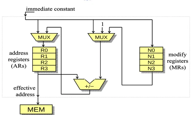
(14) Chapter 2. Backgrounds and Related Work. In this chapter, we give an overview of address generation unit in digital signal processing. Then, we will introduce the genetic algorithms. Finally, previous work related to the problem of assigning address registers to array references is presented.. 2.1 The Address Generation Unit in DSP Address code optimization is mainly used in C compilers for digital signal processors (DSPs), which require extremely high code quality and hence sophisticated code optimization techniques. Emphasis is on effective utilization of the address generation units (AGUs) commonly found in DSPs. Such an AGU generally comprises a file of address registers (ARs) as well as a file of modify registers (MRs). ARs store memory addresses (or pointers), while MRs store frequently required address modify values. The AGU architecture is sketched in Figure 2-1.. immediate constant 1 MUX MUX. address registers (ARs). MUX MUX. R0 R0 R1 R1 R2 R2 R3 R3. effective address. N0 N0 N1 N1 N2 N2 N3 N3. +/−. MEM MEM Figure 2-1 AGU Block Diagram 4. modify registers (MRs).

(15) When an address register is used to point to a memory location, the addressing mode is called “address register indirect”. The term indirect is used because the register contents are not the operand itself, but rather the address of the operand. These addressing modes specify that an operand is in memory and specify the effective address of that operand. Four general address register indirect modes are in the following. z. Auto-increment By 1 – The address of the operand is in an address register. After the operand address is used, it is incremented by 1 and stored in the same address register.. z. Auto-decrement By 1 – The address of the operand is in an address register. After the operand address is used, it is decremented by 1 and stored in the same address register.. z. Auto-increment By Offset Nn – The address of the operand is in an address register. After the operand address is used, it is incremented by the contents of a modify register and stored in the same address register. The contents of the modify register are unchanged.. z. Auto-decrement By Offset Nn – The address of the operand is in an address register. After the operand address is used, it is decremented by the contents of a modify register and stored in the same address register. The contents of the modify register are unchanged.. 2.2 Genetic Algorithms Genetic algorithms are general-purpose search algorithms based upon the principles of evolution observed in nature. The algorithms can be applied to a wide variety of optimization problems such as scheduling, computer games, stock market trading, medical, adaptive control, transportation, the traveling salesmen problem, etc. 5.

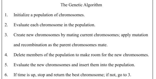
(16) The solution to a problem is called a chromosome. A chromosome is made up of a collection of genes which are simply the parameters to be optimized. A genetic algorithm creates an initial population (a collection of chromosomes), evaluates this population, and then evolves the population through multiple generations (using the genetic operators discussed below) in the search for a good solution for the problem at hand. Figure 2-2 contains a top-level description of the genetic algorithm [4] [5]. The Genetic Algorithm 1.. Initialize a population of chromosomes.. 2.. Evaluate each chromosome in the population.. 3.. Create new chromosomes by mating current chromosomes; apply mutation and recombination as the parent chromosomes mate.. 4.. Delete members of the population to make room for the new chromosomes.. 5.. Evaluate the new chromosomes and insert them into the population.. 6.. If time is up, stop and return the best chromosome; if not, go to 3. Figure 2-2 Top-level description of a genetic algorithm. 2.2.1 Selection Operators Selection is a genetic operator that chooses a chromosome from the current generation’s population for inclusion in the next generation’s population. Previous work include the following types of selection： z. Roulette – A selection operator in which the chance of a chromosome getting selected is proportional to its fitness (or rank). This is where the concept of survival of the fittest comes into play.. z. Tournament – A selection operator which uses roulette selection N times to produce a tournament subset of chromosomes. The best chromosome in this 6.

(17) subset is then chosen as the selected chromosome. This method of selection applies addition selective pressure over plain roulette selection. z. Top Percent – A selection operator which randomly selects a chromosome from the top N percent of the population as specified by the user.. z. Best – A selection operator which selects the best chromosome (as determined by fitness). If there are two or more chromosomes with the same best fitness, one of them is chosen randomly.. z. Random – A selection operator which randomly selects a chromosome from the population.. 2.2.2 Crossover Operators Crossover is a genetic operator that combines (mates) two chromosomes (parents) to produce a new chromosome (offspring). The idea behind crossover is that the new chromosome may be better than both of the parents if it takes the best characteristics from each of the parents. Crossover occurs during evolution according to a user-definable crossover probability. Previous work includes the following types of crossover. z. One Point – A crossover operator that randomly selects a crossover point within a chromosome then interchanges the two parent chromosomes at this point to produce two new offspring.. z. Two Point – A crossover operator that randomly selects two crossover points within a chromosome then interchanges the two parent chromosomes between these points to produce two new offspring.. z. Uniform – A crossover operator decides which parent will contribute each of the gene values in the offspring chromosomes.. 7.

(18) 2.2.3 Mutation Operators Mutation is a genetic operator that alters one ore more gene values in a chromosome from its initial state. It is an important part of the genetic search to prevent the population from stagnating at any local optima. Previous work include the following types of mutation. z. Flip Bit – A mutation operator that simply inverts the value of the chosen gene (0 goes to 1 and 1 goes to 0). This mutation operator can only be used for binary genes.. z. Boundary – A mutation operator that replaces the value of the chosen gene with either the upper or lower bound for that gene (chosen randomly). This mutation operator can only be used for integer and float genes.. z. Non-Uniform – A mutation operator that increases the probability that the amount of the mutation will be close to 0 as the generation number increases. This mutation operator keeps the population from stagnating in the early stages of the evolution then allows the genetic algorithm to fine tune the solution in the later stages of evolution. This mutation operator can only be used for integer and float genes.. z. Uniform – A mutation operator that replaces the value of the chosen gene with a uniform random value selected between the user-specified upper and lower bounds for that gene. This mutation operator can only be used for integer and float genes.. z. Gaussian – A mutation operator that adds a unit Gaussian distributed random value to the chosen gene. The new gene value is clipped if it falls outside of the user-specified lower or upper bounds for that gene. This mutation operator can only be used for integer and float genes.. 8.

(19) 2.2.4 Termination Methods Termination is the criterion by which the genetic algorithm decides whether to continue searching or stop the search. Each of the enabled termination criterion is checked after each generation to see if it is time to stop. Previous work include the following types of termination. z. Generation Number – A termination method that stops the evolution when the user-specified max number of evolutions have been run. This termination method is always active.. z. Evolution Time – A termination method that stops the evolution when the elapsed evolution time exceeds the user-specified max evolution time.. z. Fitness Threshold – A termination method that stops the evolution when the best fitness in the current population becomes less/greater than the user-specified fitness threshold and the objective is set to minimize/maximize the fitness.. z. Fitness Convergence – A termination method that stops the evolution when the fitness is deemed as converged. Two filters of different lengths are used to smooth the best fitness across the generations. When the smoothed best fitness from the long filter is less than a user-specified percentage away from the smoothed best fitness from the short filter, the fitness is deemed as converged and the evolution terminates.. z. Population Convergence – A termination method that stops the evolution when the population is deemed as converged. The population is deemed as converged when the average fitness across the current population is less than a user-specified percentage away from the best fitness of the current population.. z. Gene Convergence – A termination method that stops the evolution when a user-specified percentage of the genes that make up a chromosome are deemed 9.

(20) as converged. A gene is deemed as converged when the average value of that gene across all of the chromosomes in the current population is less than a user-specified percentage away from the maximum gene value across the chromosomes.. 2.3 Previous Works There are different ways of utilizing indirect addressing of AGU. One of the most popular is to perform offset assignment for local scalar variables in a C program [6][7][8]. These approaches are based on permutation of variables within available sections of memory. Hence, these techniques can not be directly applied to arrays because generally array elements are arranged in memory in order. Another important branch in address code optimization is address register assignment. Such techniques are used to assign address registers to access data for which the memory layout has been already defined. It can be directly applied to access array elements inside program loops, or to reduce the number of update instructions resulting from using offset assignment.. 2.3.1 Local Array Reference Allocation (LARA) The goal of LARA is to allocate an address register to each array reference in a basic block, by dividing them into live ranges (a live range is a set of array references that share the same address register) and assigning an address register to each range. Therefore, the final number of ranges should not exceed the total number of address registers of the processor. Moreover, the number of instructions required to redirect registers through references should be minimum. LARA has been studied before in [9][10][11][12]. These are efficient graph-based solutions, when references are restricted to basic block boundaries. In particular, Basu et al. [12] is a very efficient solution to 10.

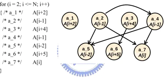
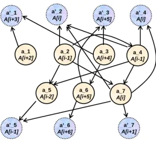
(21) LARA. In the example of Figure 2-3, array references, inside the loop on the left, are modelled as a distance graph (on the right). The distance graph G = (V, E) is a directed acyclic graph (DAG) with V = {a1 ,..., an }. The edge set E contains all edges e = (ai , a j ) with 1 ≤ i < j ≤ n . An edge e = (ai , a j ) is present in E, if using the same AR for both. ai and a j allows for generating the address for a j from the address for ai with a zero-cost address computation.. for (i = 2; i <= N; i++) { /* a_1 */ A[i+2] /* a_2 */ A[i-1] /* a_3 */ A[i+4] /* a_4 */ A[i-1] /* a_5 */ A[i-2] /* a_6 */ A[i+5] /* a_7 */ A[i] }. a_1 A[i+2]. a_2 A[i-1]. a_5 A[i-2]. a_3 A[i+4]. a_6 A[i+5]. a_4 A[i-1]. a_7 A[i]. Figure 2-3 Array references and the distance graph. In order to consider zero-cost address computation between iterations, an extended distance graph is modelled. Figure 2-4 includes inter-iteration distances in the distance. graph model of Figure 2-3. The extended distance graph is a DAG G ′ = (V ′, E ′) with V ′ = V ∪ {a1′ ,..., a n′ } , where each node ai′ ∉ V represents the array reference ai in the following loop iteration, and E ′ = E ∪ {(a j , ai′ ) | 1 ≤ i ≤ j ≤ n}. An edge (a j , ai′ ) is in E ′ , if the reference ai and a j can be implemented at zero cost using the same AR.. 11.

(22) a’_2 A[i]. a’_1 A[i+3]. a_1 A[i+2]. a’_3 A[i+5]. a_2 A[i-1]. a_5 A[i-2]. a’_5 A[i-1]. a’_4 A[i]. a_3 A[i+4]. a_6 A[i+5]. a_4 A[i-1]. a_7 A[i]. a’_7 A[i+1]. a’_6 A[i+6]. Figure 2-4 Extended distance graph. Thus, obtaining a zero overhead solution for address computation of array references in a loop with a minimum number of ARs is equivalent to covering all nodes {a1 ,..., a n } in the extended distance graph by a minimum number of node-disjoint paths P1 ,..., PK , such that if a path Pk starts in node ai it must end in node ai′ . Since this problem is NP-complete [13], the AR allocation problem is (most likely) of exponential complexity. One can compute a (potentially suboptimal) solution efficiently by the following path-based heuristic. 1.. Given a distance graph G = (V, E), construct the extended distance graph G ′ = (V ′, E ′) with V = {a1 ,..., a n } ∪ {a1′ ,..., a n′ } , and assign a unit weight to each. edge e ∈ E ′ . 2.. Let ai be the source node in {a1 ,..., a n } ⊂ V ′ with minimum index, i.e., there is no node a j with. (. (a , a )∈ E ′ j. i. and j < i . Compute the longest path. ). P = ai , ak1 ,..., akm , ai′ in G ′ between ai and ai′ . If P does not exist then stop, because no zero-cost solution is possible. 3.. Allocate a new AR for the array references represented by the nodes. {a , a i. k1. ,..., a km. }. in path P. Remove these nodes as well as the nodes 12.

(23) {a′, a′ ,..., a′ } from i. 4.. k1. km. G ′ , and remove all their incident edges.. If G ′ is not empty goto step 2, else stop and return the number r of allocated registers.. Below we show a longest path solution to the example problem. This solution results in four registers addressing the following references. R1 : a1 , a1′ R2 : a2 , a4 , a7 , a2′ R3 : a3 , a6 , a3′ R4 : a5 ,a5′. Thus the references would be R1 = &A[4] /* initialize R1 with &A[2+2] */ R2 = &A[1] /* initialize R2 with &A[2-1] */ R3 = &A[6] /* initialize R3 with &A[2+4] */ R4 = &A[0] /* initialize R4 with &A[2+2] */ for (i = 2; i <= N; i++) { /* a_1 */ *R1 ++ /* access A[i+2] /* a_2 */ *R2 /* access A[i-1] /* a_3 */ *R3 ++ /* access A[i+4] /* a_4 */ *R2 ++ /* access A[i-1] /* a_5 */ *R4 ++ /* access A[i-2] /* a_6 */ *R3 /* access A[i+5] /* a_7 */ *R2 /* access A[i] }. */ */ */ */ */ */ */. The longest path algorithm provides a tight upper bound on the number of address registers required. If the number of required address registers exceeds the number of available address registers, then the accesses allocated to some of the registers can be merged with others in a way that minimizes the incremental cost. The cost of merging 13.

(24) two ranges R and S (costÑ(R, S)) is measured by the number of update instructions required to access all array references in the resulting range. The process of merging is iteratively performed till the number of address registers required equals the number of available registers. The pseudo-code for the MERGE algorithm is shown below.. (1) procedure MERGE (R, nars). (2). while |R| > nars do. (3). mincost » +∞. (4). for each range R ∈ R do. (5). for each range S ∈ R, S ≠ R do. (6). if costÑ(R, S) < mincost then. (7). mincost » costÑ(R, S). (8). minpair » {R, S}. (9). R » (R – minpair) ∪ (R Ñ S). On applying the path merging approach to the longest path solution, shown earlier, subjected to the constraint of three available address registers, we obtain the following solution with one inserted address-modifying instruction. Here, the accesses by registers R1 and R2 has been merged. The costs stem from transitions from references a5 to a7 in register R2. R1 : a1 , a1′ R2 : a2 , a4 , a5 , a7, a2′ R3 : a3 , a6 , a3′. The address register allocation technique shown in the beginning of this section is a polynomial-time procedure. It utilizes two algorithms, the FIND_TUB (find tight upper bound) algorithm to compute the minimum number of registers and the MERGE 14.

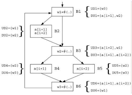
(25) algorithm of combining the paths. The first algorithm is of complexity O (| V |2 ⋅ | E |), where V and E denote respectively the vertex and edge sets of the extended distance graph. The Path-Merge-Cost procedure of MERGE is of linear complexity in the number n of array accesses, while the invocation of this procedure by MERGE is bounded by O(n 2 ) . Hence, the worst case complexity of MERGE is O (n 3 ) . Since. ( ). V = O(n ) , the total runtime is dominated by FIND_MIN and is in O n 4 . In practice. this means, that the computation time is in within the range of CPU milliseconds on a SparcStation-10.. 2.3.2 Global Array Reference Allocation (GARA) The problem of assigning address registers to array references, across basic blocks, is known as Global Array Reference Allocation (GARA). It has been studied before in [14][15] finding solutions for the allocation of address registers for a whole procedure. Consider, for example, the CFG fragment shown in Figure 2-5, after Ø-equations are inserted into blocks B1, B3 and B6. The UD and DU sets for all basic blocks that perform array references are shown in Figure 2-5. We assume here that the program begins (ends) before (after) block B1 (B6). Notice that, if Ø-equations had not been inserted, the instructions associated to reference a[i + 1] in B2 would be reached (across one loop iteration) by two references, that is, UD2 = {a[i + 1], a[i + 2]}. In this case, it would not be possible to determine, at compile time, which of these two references reach a[i + 1], and hence if auto-increment mode could be used by their instructions to point to a[i + 1]. After Ø-equations are inserted, the ud-chain at B2 becomes UD2 = {w1}, only one reference reaches a[i + 1], and thus the decision can made once the value for w1 is computed.. 15.

(26) Figure 2-5 CFG fragment after Ø-insertion and reference analysis. 2.3.3 Summary of Address Code Optimization with AGU There are mainly two ways of utilizing auto-increment addressing modes: Offset Assignment and Address Register Assignment. All of them reduce addressing costs. further by assignment of multiply required modify values to MRs in a post-pass phase. Table 2-1 shows comparison of related work and our problem. We will propose two approaches to LARA with MR Optimization which consider modify register when doing AR optimization. The methodology will describe more detailed in next chapter.. 16.

(27) Table 2-1 Comparison of related work and our problem. Year. Problem Domain. Leupers [6]. 1996. Offset Assignment. Basu [12]. 1999. AR Assignment: LARA. Araujo [15]. 2002. AR Assignment: GARA. Our problem. MR Optimization. AR Assignment: LARA. 17. After AR optimization. Consider MR when AR optimization.

(28) Chapter 3. Proposed Methods. In this chapter, we give an observation of benefit of considering modify register when doing AR optimization. Then problem description and problem transformation based on Basu’s graph are presented. Finally, we propose two methods to solve this problem in detail.. 3.1 Observation Consider the following array references with respect to some array A. for (i = 2; i <= N; i++) { /* a_1 */ A[i-6] /* a_2 */ A[i-5] /* a_3 */ A[i] /* a_4 */ A[i+2] /* a_5 */ A[i+5] /* a_6 */ A[i+6] /* a_7 */ A[i+1] }. If two ARs are available, Basu’s approach to find minimum addressing costs would be in the following processes. 1.. Estimate the upper bound of the number of ARs required to ensure all address computation of array elements can be handle by auto-inc/dec.. 2.. If the number of registers obtained exceeds the given constraint on the set of available registers, adopt MERGE algorithm.. 18.

(29) The result of the example needs three addressing costs. R1 = &A[0] R2 = &A[6] for (i = 6; i <= N; i++) { /* a_1 */ *R1 ++ /* a_2 */ *R1 R1 += 10 /* a_3 */ *R2 R2 += 2 /* a_4 */ *R2 -/* a_5 */ *R1 ++ /* a_6 */ *R1 R1 += 11 /* a_7 */ *R2 }. Now if two MRs are available, we intuitively consider the usage of multiple modify registers that store frequently modify values for AR updates. The final result of the example needs one addressing cost. R1 = &A[0] R2 = &A[6] N1 = 10 N2 = 2 for (i = 6; i <= N; i++) { /* a_1 */ *R1 ++ /* a_2 */ *R1 += N1 /* a_3 */ *R2 += N2 /* a_4 */ *R2 -/* a_5 */ *R1 ++ /* a_6 */ *R1 R1 += 11 /* a_7 */ *R2 }. However, this is not the best solution when two ARs and two MRs are given. If we 19.

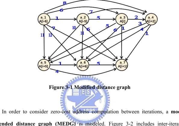
(30) know which values should be stored in MRs, some edges can be added in Basu’s. extended distance graph so that there may be an opportunity to find fewer path cover of the extended distance graph. The best result of above example need zero addressing cost. R1 = &A[0] R2 = &A[8] N1 = 5 N2 = 6 for (i = 6; i <= N; i++) { /* a_1 */ *R1 ++ /* a_2 */ *R1 += N1 /* a_3 */ *R1 += N1 /* a_4 */ *R2 ++ /* a_5 */ *R1 ++ /* a_6 */ *R1 -= N1 /* a_7 */ *R1 -= N2 }. 3.2 Problem Description The problem of addressing code optimization with AGU can now be stated as follows: Given: a set of address registers R = {ri | 1 ≤ i ≤ k } , a set of modify registers. M = {mi | 1 ≤ i ≤ l} , and array reference pattern A = {ai | 1 ≤ i ≤ n} , where each ai is an ordered pair (of i , csi ) , of i denoting the index of an array referred at control step csi . Required: an allocation of all elements of A to the elements of R such that the addressing. costs in a loop which can not be handled by auto-inc/dec and l auto-modify is minimized.. 3.3 Problem Transformation We first model our distance graph. The modified distance graph G = (V, E, d) is a directed acyclic graph (DAG) with V = {a1 ,..., an }. The edge set E contains all edges 20.

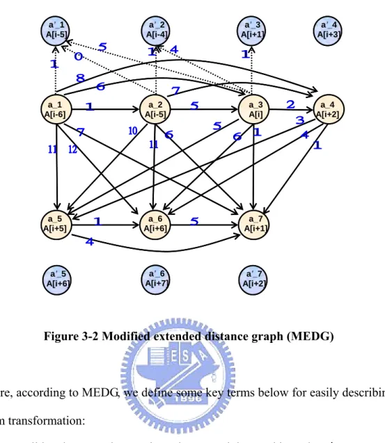
(31) e = (ai , a j ) with 1 ≤ i < j ≤ n and the d = (ai , a j ) denotes | of j − of i | . Figure 3-1 shows the modified distance graph for our above example loop. Edges don’t represent auto-inc/dec any more. On the contrary, values on the edges (excluding 0 and 1) represent the candidate to be assigned to modify registers.. a_1 A[i-6]. a_2 A[i-5]. a_3 A[i]. a_5 A[i+5]. a_6 A[i+6]. a_7 A[i+1]. a_4 A[i+2]. Figure 3-1 Modified distance graph. In order to consider zero-cost address computation between iterations, a modify extended distance graph (MEDG) is modeled. Figure 3-2 includes inter-iteration. distances in the modified distance graph model of Figure 3-1. The modified extended distance graph is a DAG G ′ = (V ′, E ′, d ) with V ′ = V ∪ {a1′ ,..., a n′ } , where each node ai′ ∉ V. represents the array reference ai in the following loop iteration, and. E ′ = E ∪ {(a j , ai′ ) | 1 ≤ i ≤ j ≤ n} (some edges are ignored in Figure 3-2 for clarity). d = (ai , a j ) denotes | of j − of i | and d = (a j , ai' ) denotes of i + step − of j . Values on the edges represent the candidate to be assigned to modify registers.. 21.

(32) a’_1 A[i-5]. a’_2 A[i-4]. a’_3 A[i+1]. a’_4 A[i+3]. a_1 A[i-6]. a_2 A[i-5]. a_3 A[i]. a_4 A[i+2]. a_5 A[i+5]. a_6 A[i+6]. a_7 A[i+1]. a’_6 A[i+7]. a’_7 A[i+2]. a’_5 A[i+6]. Figure 3-2 Modified extended distance graph (MEDG). Here, according to MEDG, we define some key terms below for easily describing our problem transformation: z. a valid path P: a path starts in node ai and then end in node ai′. z. k disjoint valid paths P1 ,..., Pk : these k paths cover all nodes {a1 ,..., a n } exactly once.. z. D( P1 ,..., Pk ): a set of differences in these k paths. z. countd( P1 ,..., Pk ): number of difference d in these k paths. If P1 ,..., Pk is explicit, we refer it as count(d).. z. costl( P1 ,..., Pk ): consider the usage of l MRs, the addressing costs in a loop is defined as | D|. costl( P1 ,..., Pk ) =. ∑ count (d ) − count (1) − count (0) − ∑ l maximum count(d) i =1. i. 22.

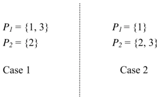
(33) For example, according to Figure 3-2, P1 = {1, 3, 6, 1′ }, P2 = {2, 4, 2′ }, and P3 = {5, 7, 5′ } are three disjoint valid paths. D(P1, P2, P3) = {4, 5, 6, 7, 11}. count(4), count(5), count(6), count(7), and count(11) are 1, 1, 3, 1, and 1 respectively. If l is two, then 5. cost2(P1, P2, P3) =. ∑ count (d ) − count (1) − count (0) − ∑ 2 maximum count(d) i =1. i. = [count(4) + count(5) + count(6) + count(7) + count(11)]. − count (1) − count (0) − [ ∑ 2 maximum count(d)] = [1 + 1 + 3 + 1 + 1] – 0 – 0 – [3 + 1] =3 Thus, the problem of obtaining a minimum number of addressing costs in a loop if k ARs and l MRs are given is equivalent to finding k disjoint valid paths P1 ,..., Pk in the MEDG such that costl( P1 ,..., Pk ) is minimal.. 3.4 Approach 1: Brute Force with Pruning We iteratively search all combinations of P1 ,..., Pk in the MEDG and prune some cases which are far away from optimal solution to decrease computation time. For example, Figure 3-3(a) is a source program and Figure 3-3(b) is its MEDG.. for (i = 2; i <= N; i++) { /* a_1 */ A[i-2] /* a_2 */ A[i+1] /* a_3 */ A[i+4] /* a_4 */ A[i+1] }. a’_1 A[i-1]. a’_2 A[i+2]. a’_3 A[i+5]. a’_4 A[i+2]. a_1 A[i-2]. a_2 A[i+1]. a_3 A[i+4]. a_4 A[i+1]. (a). (b) Figure 3-3 (a) A source program (b) MEDG 23.

(34) If two ARs and one MR are available, our goal is to divide array reference pattern into two paths such that cost1(P1, P2) is minimum. Initially, we set P1 = {1}, and an upper bound UB = 1 which is cost1(P1, P2) where (P1, P2) is obtained from Basu’s approach. Then, we consider array references from node 2 one by one. Each node can be put in either existing paths or, if the number of existing paths is less than k, we can create a new path to put the node in. Figure 3-4 shows there are two cases when we consider node 2.. P1 = {1, 2}. P1 = {1} P2 = {2}. Case 2. Case 1. Figure 3-4 Two cases when considering node 2. After a node is added in a path, we compute its corresponding costl( P1 ,..., Pk ). If the cost is greater than or equal to current upper bound, we prune further search and consider other cases. Otherwise, if the cost is less than current upper bound, we continue the next node. For example, cost1(P1, P2) of case 1 in Figure 3-4 is zero. We can continue the node 3 because the cost is less than current upper bound. So, there are also two cases when we consider node 3 like Figure 3-5. Of course, we can not create a new path for node 3 because there are only two ARs available.. P1 = {1, 3} P2 = {2}. P1 = {1} P2 = {2, 3} Case 2. Case 1. Figure 3-5 Two cases when considering node 3 of case 1 in Figure 3-4 24.

(35) If all nodes are settled in k paths, we put ai′ to the tail of each path, where ai is the head of its corresponding path. Then, if cost1( P1 ,..., Pk ) is less than current upper bound, we update the current upper bound. When all cases are considered, we output the upper bound as the final result. For example, cost1(P1, P2) of case 1 in Figure 3-5 is zero. So, there are also two cases when we consider node 4. Figure 3-6 shows two cases when all nodes are considered, and cost1(P1, P2) of case 1 and cost1(P1, P2) of case 2 are two and one respectively. So, it is not necessary to update the current upper bound.. P1 = {1, 3, 4, 1′ } P2 = {2, 2′ }. P1 = {1, 3,1′ } P2 = {2, 4, 2′ } Case 2. Case 1. Figure 3-6 Two cases when considering node 4 of case 1 in Figure 3-5. It is like traversing a tree using depth first search if we display all combination of above example in Figure 3-7. Although this is a time-consuming approach, some sub-tree can be pruned when traversing because of the upper bound. This may save much runtime in most cases.. 25.

(36) node 1. node 2. node 3. P1 = {1, 3} P2 = {2} P1 = {1} P2 = {2}. P1 = {1} P2 = {2, 3}. node 4. P1 = {1, 3, 4, 1′ } P2 = {2, 2′ } P1 = {1, 3,1′ } P2 = {2, 4, 2′ } P1 = {1, 4, 1′ } P2 = {2, 3, 2′ } P1 = {1, 1′ } P2 = {2, 3, 4, 2′ }. P1 = {1} P1 = {1, 2, 3, 4,1′ } P1 = {1, 2, 3} P1 = {1, 2, 3, 1′ } P2 = {4, 4′ } P1 = {1, 2}. P1 = {1, 2} P2 = {3}. P1 = {1, 2, 4, 1′ } P2 = {3, 3′ } P1 = {1, 2, 1′ } P2 = {3, 4, 3′ }. Figure 3-7 All combination of above example. After knowing the concept of pruning method, we give a pseudo algorithm described below showing how to traverse this tree and finally obtain an optimal solution.. 26.

(37) 1.. //INPUT: k ARs, l MRs, and array reference pattern A = {ai | 1 ≤ i ≤ n}. 2.. //OUTPUT: costl( P1 ,..., Pk ). 3.. Build MEDG according to A. 4.. Initial UB to costl( P1 ,..., Pk ), where P1 ,..., Pk is obtained from Basu’s approach.. 5.. Initial P1 = { a1 }, Pi = {Ø} for 2 ≤ i ≤ k. 6.. call DFS(2). 7.. output UB. The algorithm receives k ARs, l MRs, and array reference pattern as input, and builds MEDG in line 3. Line 4 and 5 initiate UB for pruning and a1 is put in P1. DFS function is to create and traverse this tree, and the parameter 2 means we begin to consider a 2 . After line 6 is done, we get UB as an optimal solution. Now we present the algorithm DFS, which is a recursive call.. 1.. DFS(i) {. 2.. Either tail ai to any one of existing paths or, if existing paths is less than k, create a new path of which ai is the head.. 3.. for each case P1 ,..., Pk { if (i == n) {. 4. 5.. add a′j to each P where a j is the head of P. 6.. if (costl( P1 ,..., Pk ) < UB) update UB to costl( P1 ,..., Pk ). 7.. }. 8.. else if (costl( P1 ,..., Pk ) < UB) DFS(i + 1). 9.. }. 10. } 27.

(38) Line 2 in DFS algorithm indicates there are at most k cases when we put ai to. P1 ,..., Pk . Line 4-7 means if all nodes are considered, we add a′j to each P where a j is the head of P and update UB according to costl( P1 ,..., Pk ). Line 8 is the main idea of pruning method: only costl( P1 ,..., Pk ) < UB is possible to approach optimal solution and it is necessary to consider ai +1 .. 3.4.1 Time Complexity ⎛ kn ⎞ The time complexity of trying every combination of P1 ,..., Pk is O⎜⎜ ⎟⎟ , where n is ⎝ k! ⎠. number of array references and k is number of ARs (We can consider this problem as computing combinations of putting n different balls into k identical baskets. These baskets can be either full or empty, but the sum of balls in these baskets is n). Then the time complexity of computing costl( P1 ,..., Pk ) is O( E log E ) , because we have to sort the differences in P1 ,..., Pk and the number of these differences are not more than the number of edges in MEDG. Since E = O (n 2 ) , the total time complexity of worst case is ⎛ kn 2 O⎜⎜ n log n 2 k ! ⎝. (. )⎞⎟⎟ . Although pruning method can reduce computation time, there is a ⎠. limit if n is large. Therefore, in the next section we will propose genetic algorithm which can solve problems with large n in a short time.. 28.

(39) 3.5 Approach 2: Genetic Algorithm (GA) Genetic Algorithm (GA) is an adaptive heuristic search algorithm premised on the evolutionary ideas of natural selection and genetic. The basic concept of GAs is designed to simulate processes in natural system necessary for evolution, specifically those that follow the principles first laid down by Charles Darwin of survival of the fittest. As such they represent an intelligent exploitation of a random search within a defined search space to solve a problem.. 3.5.1 Overview of GA We choose GA for solving LARA problem mainly due to some reasons: First, this problem is very complicated and no polynomial time algorithm can solve it. Second, if enough computation time is invested, GA approximates a global optimum much more likely than heuristics which are trapped in a local optimum. Third, this problem has a straightforward encoding as a GA, and the complexity of computing the fitness of a chromosome is also bounded in polynomial time. We choose steady-state genetic algorithm that uses overlapping populations. In this variation, we initialize a population with certain number of chromosomes (m chromosomes for example). Then, two chromosomes in the population are selected to produce another m offsprings. In order to maintain m chromosomes in the population, we replace worse members in original population with new offsprings. Figure 3-8 illustrates the flow chart of our GA.. 29.

(40) Initialize population randomly. Select chromosome randomly for mating. Apply crossover and mutation as the parent mate. Delete members of the population to make room for the new chromosome. Evaluate the new chromosome and insert them into the population N. Are stopping criteria satisfied? Y Finish Figure 3-8 Flow chart of our GA. Throughout the rest of this section, we will use the terms “solution,” “individual,” and “chromosome” interchangeably to refer to either costl( P1 ,..., Pk ) where P1 ,..., Pk is a certain combination in searching space or its representation in the GA.. 3.5.2 Chromosomal Representation The basic idea of encoding as a chromosome is to determine the most important values to be stored in MRs. If we choose these values properly, it will reduce many addressing costs. Therefore, the length of a chromosome is the total number of different difference (excluding 0 and 1) in MEDG and each gene in a chromosome corresponds to a difference respectively and it is either ‘0’ or ‘1’. For example, Figure 3-9(c) shows there are five genes in a chromosome because total number of different difference in Figure 30.

(41) 3-9(b) is five (They are 3, 6, 2, 5, and 4). Thus, gene 1 may correspond to 3, gene 2 may correspond to 6, gene 3 may correspond to 2, gene 4 may correspond to 5 and gene 5 may correspond to 4. for (i = 2; i <= N; i++) { /* a_1 */ A[i-2] /* a_2 */ A[i+1] /* a_3 */ A[i+4] /* a_4 */ A[i+1] }. a’_1 A[i-1]. a’_2 A[i+2]. a’_3 A[i+5]. a’_4 A[i+2]. a_1 A[i-2]. a_2 A[i+1]. a_3 A[i+4]. a_4 A[i+1]. (a). (b). 3. 6. 2. 5. 4. Chromosome. gene 1. gene 5 (c). Figure 3-9 (a) a source program (b) MEDG (c) chromosome representation. 3.5.3 Population Initialization If k ARs and l MRs are available, we initialize a population with m chromosome. Each chromosome contains l ‘1’s and other genes in chromosome are ‘0’. This constraint may speed up computation time of convergence (we will discuss this later). Figure 3-10 is an example that if two ARs and two MRs are available, two ‘1’s exist in each chromosome. 31.

(42) Initial population Chromosome 1. 1 0 1 0 0. . . . Chromosome m 0 1 0 1 0. Figure 3-10 An example of initial population. 3.5.4 Crossover and Mutation Operation We apply one-point crossover operation to produce offspring from two selected parents in the population and apply bit mutation operation to each individual of the offspring.. One-point crossover operation. After two parents are selected (Figure 3-11(a)), we randomly specify a point on these two chromosomes (Figure 3-11(b)). Then we interchange their tail from the point and produce two new offsprings (Figure 3-11(c)).. Bit mutation operation. Each gene of produced chromosomes has probability to flip bit from ‘0’ to ‘1’ or from ‘1’ to ‘0’. Figure 3-12 shows an example that gene 3 and gene 5 are mutated within a chromosome.. 32.

(43) Parent 1:. 0. 1. 1. 0. 0. Parent 2:. 0. 1. 0. 1. 0. (a). one point Parent 1:. 0. 1. 1. 0. 0. Parent 2:. 0. 1. 0. 1. 0. Child 1:. 0. 1. 1. 1. 0. Child 2:. 0. 1. 0. 0. 0. (b). (c). Figure 3-11 One-point crossover operation. Before mutating. 0. 1. 1. 1. 0. After mutating. 0. 1. 0. 1. 1. Figure 3-12 Bit mutation operation. Notice that we constrain the number of ‘1’ within a chromosome initially. However, after applying crossover and mutation operation, the number of ‘1’ may not equal to l. We will discuss this situation later. 33.

(44) 3.5.5 Evaluation Function The genetic algorithm uses an objective function to determine how 'fit' each chromosome is for survival. We evaluate the fitness of a chromosome according to the following steps: 1.. Some edges in the MEDG are removed if the genes corresponding to difference of the edges indicate ‘0’.. 2.. Apply Basu’s heuristic to obtain k paths P1 ,..., Pk. 3.. Evaluation function of the chromosome = costl( P1 ,..., Pk ). In our design, smaller the fitness of the chromosome is, higher score it has. That is, it is more possible to stay in the population. Take Figure 3-9 for example. Two ARs and two MRs are available and we want to calculate the fitness of the chromosome in Figure 3-13(a). According to the chromosome, we remove edges in Figure 3-9(b), which differences are 3 and 2 because genes corresponding to 3 and 2 in the chromosome are ‘0’ (see Figure 3-13(b)). Then we apply Basu’s approach: Figure 3-13(c) shows two ARs are needed in phase 1 and MERGE algorithm is not necessary to applied because we have exactly two ARs available. So, the paths are P1 = {a1, a3, a1′ } and P2 = {a2, a4, a ′2 }. Finally, the fitness of the chromosome is cost2(P1, P2) or zero. This is a good way to encode and decode a chromosome because edges should be kept in the graph tend to “evolve” genes to 1 and those should removed tend to evolve to 0. These differences on the edges are addressing costs but only l MRs can handle them. Therefore, we constrain the number of ‘1’ within a chromosome at the beginning of the population. However, in the process of crossover and mutation operation, we permit the number of ‘1’ within a chromosome being unequal to l. This may also peed up computation time of convergence. For example, there are three ‘1’s within the chromosome in Figure 3-13(a) and gene 5 does not influence the fitness of the 34.

(45) chromosome — whether it is ‘0’ or ‘1’. However, leaving the gene 5 to ‘1’ may have a good effect on next generation. In fact, from our experiment, we get better solution if we constrain the number of ‘1’ within a chromosome at the beginning of the initial population and allow it to be unequal in the process of crossover and mutation operation.. (a) Chromosome. 3. 6. 2. 5. 4. 0. 1. 0. 1. 1. (b). (c). a’_1 A[i-1]. a’_2 A[i+2]. a’_3 A[i+5]. a’_4 A[i+2]. a_1 A[i-2]. a_2 A[i+1]. a_3 A[i+4]. a_4 A[i+1]. a’_1 A[i-1]. a’_2 A[i+2]. a’_3 A[i+5]. a’_4 A[i+2]. a_1 A[i-2]. a_2 A[i+1]. a_3 A[i+4]. a_4 A[i+1]. Figure 3-13 An example of calculating a chromosome of evaluation function. 35.

(46) 3.5.6 Parameters We select the following parameters: Population size: 30 individuals Mutation probability per gene: 1/n, where n is number of array references Replacement rate: 2/3 of the population size Termination condition: 2000 generations or conservative 500 generations without a. fitness improvement. 3.5.7 Time complexity The time complexity of evaluating a chromosome is O(n 4 + n 2 log n 2 ) where n 4 is FIND-MIN algorithm to find a case of P1 ,..., Pk and n 2 log n 2 is to compute. costl( P1 ,..., Pk ). Because n 2 log n 2 is smaller than n 4 , the time complexity of evaluating a chromosome is dominated by O(n 4 ) . If there are m chromosomes in a population and. L generations are produced, the total time complexity is O( L ⋅ m ⋅ n 4 ) .. 36.

(47) Chapter 4. Simulation and Analysis. In this chapter, we introduce the benchmark programs. Then we compare the addressing costs in loops of GA and pruning method to Basu’s approach when ARs and MRs are given different numbers. Finally, we give a summary of experimental results.. 4.1 Benchmark Suite In order to evaluate the efficiency of using the AGU, we introduce the stencil Micro-Benchmark Suite. Stencil codes continue to play an important role in scientific computations as well as the fields of image processing and geometric modeling. Each program contains a loop kernel with a sequence of accessing the same array references. They are taken from three sources. All the integer stencils can be found in a book on image processing [16]. The floating point stencils come from the domain of partial differential equations [17] and the NAS MG Parallel Benchmark [18][19]. These kernels are listed in Table 4-1. The type is given by the first letter of the benchmark name: “D” for floating point and “I” for integer codes. The 2D stencil kernels are run over a 1000 by 1000 array of floating point or integer values; the 3D stencil kernels over a 100 by 100 array.. 37.

(48) Table 4-1 Stencil Micro-Benchmarks Suite Benchmark. # of array references Usage. DISO3X3 DROW3X3 INOISE1 IPREWITT ISOBEL IYOKOI DLILBIHARM DRPRJ3(3D) DRESID(3D) IMORPH IROBINSON DBIGBIHARM DISO5X5 INOISE2 ILINEDET INOISE3 IWIDELINEDET IBIGLAPLACE INEVATIA IZEROCROSS. 9 9 9 12 12 12 13 19 21 21 24 25 25 25 48 49 72 97 141 211. Biharmonic operator Partial derivatives Partial derivatives Biharmonic operator NAS MG Benchmark Partial derivatives NAS MG Benchmark Gradient edge detection Line detection Mathematical morphology Gradient edge detection Noise cleaning Noise cleaning Noise cleaning Edge detection Gradient edge detection Edge detection Wide line detection Connectivity number Edge detection. 4.2 Experimental Results Three approaches are implemented in C++ and tested on desktop computer with an Intel Pentium 4 2.4GHz processor and 1.0GB RAM, running under Linux 2.4.22. For each program in Stencil Micro-Benchmarks Suite, we run the GA 10 times to examine the algorithm’s performance. Under a variety of ARs and MRs, our experiment is divided into two parts. One is comparison of addressing costs between Basu’s approach, GA and pruning method for small programs which number of array references are smaller than 49. This is because 38.

(49) pruning method can not find the optimal solution in one day for those programs which number of array references are greater than 49. The other is comparison of addressing costs between Basu’s approach and GA for all programs. In each figure of the simulation results, the X-axis is a fixed number of ARs and different number of MRs. The Y-axis is the total addressing costs for small programs which number of array references is smaller than 49, or for all programs. Each configuration of AR and MR has three bars, indicating three (two) approaches: Basu, GA and Pruning (only for small programs). From these figures we can see that GA and Pruning perform better than Basu’s approach except for Figure 4-1 and Figure 4-5. This is because the only solution for one AR given to access n array references is P1 = { a1 ,..., an , a1′ }. Therefore, these three approaches have same addressing costs for small (all) programs. Table 4-2 and Table 4-3 show the reduction rate of addressing costs based on Basu’s approach. We can see that under fixed number of ARs, our approaches can perform better than Basu’s when given more MRs.. For small programs 200 Addressing Costs. z. Basu GA. 150. Pruning 100 50 0 1AR1MR. 1AR2MR. 1AR3MR. 1AR4MR. Figure 4-1 Addressing costs of 1 AR and l MRs for small programs. 39.

(50) Addressing Costs. 160. Basu. 140. GA. 120. Pruning. 100 80 60 40 20 0 2AR1MR. 2AR2MR. 2AR3MR. 2AR4MR. Figure 4-2 Addressing costs of 2 ARs and l MRs for small programs. 120. Basu. Addressing Costs. 100. GA Pruning. 80 60 40 20 0 3AR1MR. 3AR2MR. 3AR3MR. 3AR4MR. Figure 4-3 Addressing costs of 3 ARs and l MRs for small programs. 80. Basu. Addressing Costs. 70. GA. 60. Pruning. 50 40 30 20 10 0 4AR1MR. 4AR2MR. 4AR3MR. 4AR4MR. Figure 4-4 Addressing costs of 4 ARs and l MRs for small programs. 40.

(51) Table 4-2 Addressing costs reduction for small programs. GA. Pruning 1 MR. GA. Pruning. GA. 2 MRs. Pruning. 3 MRs. GA. Pruning. 4 MRs. 2 ARs. 30%. 33%. 44%. 48%. 58%. 59%. 67%. 72%. 3 ARs. 35%. 41%. 51%. 58%. 63%. 67%. 74%. 82%. 4 ARs. 30%. 39%. 47%. 62%. 72%. 83%. 85%. 91%. For all programs. 600 Basu Addressing Costs. 500. GA. 400 300 200 100 0 1AR1MR. 1AR2MR. 1AR3MR. 1AR4MR. Figure 4-5 Addressing costs of 1 ARs and l MRs for all programs 500 Basu Addressing Costs. z. 400. GA. 300 200 100 0 2AR1MR. 2AR2MR. 2AR3MR. 2AR4MR. Figure 4-6 Addressing costs of 2 ARs and l MRs for all programs 41.

(52) 500 Addressing Costs. Basu 400. GA. 300 200 100 0 3AR1MR. 3AR2MR. 3AR3MR. 3AR4MR. Figure 4-7 Addressing costs of 3 ARs and l MRs for all programs. 400 Addressing Costs. Basu GA. 300 200 100 0 4AR1MR. 4AR2MR. 4AR3MR. 4AR4MR. Figure 4-8 Addressing costs of 4 ARs and l MRs for all programs. Table 4-3 Addressing costs reduction for all programs. GA 1 MR. 2 MRs. 3 MRs. 4 MRs. 2 ARs. 26%. 33%. 39%. 43%. 3 ARs. 32%. 41%. 49%. 56%. 4 ARs. 29%. 37%. 49%. 56%. 42.

(53) 4.2.1 Summary of Experimental Results For small programs, GA reduces 55% addressing costs in average compared to Basu’s approach while pruning method reduces 61%. Therefore, comparing its results to the optimal solutions, GA performs very well with an average overhead of less than 6%. Besides, GA runs less than five minutes for each program (including large programs). For all programs, GA reduces 41% addressing costs in average compared to Basu’s approach.. 43.

(54) Chapter 5. Conclusion and Future Works. In this thesis, we have proposed approaches for optimizing array index computation targeted to the DSP processors with auto-increment (decrement) by 1 and auto-modify features under register constraints. If program size is small, we can apply pruning method to find optimal solution while program size is large, we apply GA to obtain a reasonable solution. Experimental results show that our approaches are indeed very effective in comparison with Basu’s method. Unlike previous research which emphasizes the usage of auto-increment (decrement) by 1, our results show that a good decision of clustering array references into ARs makes addressing costs minimized. There are still some researches could be further studied. First, a more precise method to evaluate program performance improvement is required. We will try to integrate our optimizations into DSP compilers and analyze the execution cycles. Second, we will consider basic blocks. Not much work has been done toward finding solutions for the allocation of address registers across basic blocks. Finally, there are some special indirect addressing modes in certain DSPs. More techniques are required to exploit.. 44.

(55) References [1]. P. Paulin, M. Cornero, C. Liem, et al. “Trends in Embedded Systems Technology”, in: M.G. Sami, G. De Micheli (eds.): Hardware/Software Codesign, Kluwer Academic Publishers, 1996 [2]. V. Zivojnovic, J.M. Velarde, C. Schläger, H. Meyr, “DSPStone – A DSP-oriented. Benchmarking Methodology”, Int. Conf. on Signal Processing Applications and Technology (ICSPAT), 1994 [3]. P. Marwedel, G. Goossens (eds.), “Code Generation for Embedded Processors”, Kluwer Academic Publishers, 1995 [4]. L. Davis, “Hand book of Genetic Algorithms”, Van Nostrand Reinhold, 1991 [5]. Genetic Server and Genetic Library. 2001. The NeuroDimension company. http://www.nd.com/genetic/ [6]. R. Leupers and P. Marwedel, “Algorithm for address assignment in DSP code generation”, in Proc. Int. Conf. Computer-Aided Design, pp.109-112, 1996. [7]. S. Atri, J, Ramanujam, M. Kandemir, ”Improving Offset Assignment for Embedded Processors”, Languages and Compiler for High-Performance Computing, S. Midkiff et al. (eds.), Lecture Notes in Computer Science, Springer, 2001. [8]. Rainer Leupers, “Offset Assignment Showdown：Evaluation of DSP Address Code. Optimization Algorithms”, Institute for Integrated Signal Processing System (ISS), 2003. [9]. G. Araujo, A. Sudarsanam, S. Malik, “Instruction Set Design and Optimizations for Address Computation in DSP Architectures”, 9th Int. Symp. On System Synthesis (ISSS), 1996 [10]. R. Leupers, A. Basu, and P. Marwedel, “Optimized Array Index Computation in DSP Programs”, Proc. Asia and South Pacific Design Automation Conference, February 45.

(56) 1998 [11]. G. Araujo, S. Malik, “Register Allocation for Indirect Addressing in Loops”, 1998 [12]. Basu, A., Leupers, R., and Marwedel, P. 1999. “Array index allocation under register constraints in DSP programs”. In proceedings of the International Conference on VLSI Design. IEEE Press, Los Alamitos, CA. [13]. N. Robertson, P.D. Seymour, “An outline of Disjoint Path Algorithms”, pp. 267-292 in: B. Korte, L. Lovasz, H.J. prömel, A. Schrijver (eds.): Paths, Flows, and VLSI Layout, Springer-Verlag, 1990 [14]. M. Cintra, G. Araujo, “Array Reference Allocation Using SSA-Form and Live Range Growth”, LCTES, 2000 [15]. G. Araujo, G. Ottoni, “Global Array Reference Allocation”, ACM Transactions on Design Automation of Electronic Systems, Vol. 7, No. 2, April 2002 [16]. R. M. Haralick and L. G. Shapiro, “Computer and Robot Vision”, Addison-Wesley, 1992 [17]. M. Abramowitz and I. A. Stegun, “Handbook of mathematical functions, with formulas, graphs, and matheatical tables”, Dover Publications, 1973 [18]. D. Bailey, E. Barszca, J. Barton, D. Browning, R. Carter, L. Dagum, R. Fatoohi, S. Fineberg, P. Frederickson, T. Lasinski, R. Schreiber, H. Simon, V. Venkatakrishnan, and S. Weeratunga. The NAS parallel benchmarks (94). Technical report, RNR Technical Report RNR-94-007, March 1994 [19]. D. Bailey, T. Harris, W. Saphir, R. van der Wijngaart, A. Woo, and M. Yarrow. The NAS parallel benchmarks 2.0. Technical report, NAS Report NAS-95-020, December 1995. 46.

(57)