兩個逆高斯分配的平均值及尺度參數之廣義推論

國 立 交 通 大 學

統計學研究所

碩 士 論 文

兩個逆高斯分配的平均值及尺度參數之廣義推論

Generalized inferences on the means and scales of

two independent Inverse Gaussian populations

研 究 生 ： 林孟樺

指導教授 ： 李昭勝 博士

林淑惠 博士

兩個逆高斯分配的平均值及尺度參數之廣義推論

Generalized inferences on the means and scales of

two independent Inverse Gaussian populations

研 究 生： 林孟樺

Student: Meng-Hua

Lin

指導教授： 李昭勝 博士

Advisors: Dr. Jack C. Lee

林淑惠 博士

Dr. Shu-Hui Lin

國 立 交 通 大 學

統計學研究所

碩 士 論 文

Institute of Statistics

National Chiao Tung University

June 2006

i

兩個逆高斯分配的平均值及尺度參數之

廣義推論

研究生：林孟樺 指導教授： 李昭勝 博士

林淑惠 博士

國立交通大學統計學研究所

摘要

逆高斯分配在分析全為正數且右偏的數據時是一個很好的模型，因

此在統計應用上很受重視。過去的研究中，在不假設干擾參數相等的情

況下比較兩個母體的平均值及尺度參數的推論還需要我們繼續研究。因

此在本論文中，我們利用廣義p值法對於一個及兩個逆高斯分配母體參

數尋求精確的檢定方法，並提出一個在使用上比過去更為便利的方法，

而這個方法是建立在廣義方法的觀念上，解決了在使用過去文獻中檢定

兩個母體平均值的比例和計算信賴區間時會遇到的困難，也就是統計量

中包含了干擾參數的問題，而且我們也得到了確切的解。藉由實際數據

的分析，我們發現我們的方法跟過去的方法比較起來可以得到長度最短

或是很接近最短的信賴區間長度。並且在模擬的研究中，我們可以看出

我們的方法所得出的覆蓋率與型I誤差都很接近我們所設定的水準。

關鍵字：覆蓋率；期望長度；廣義信賴區間；廣義p值；型I誤差

ii

Generalized inferences on the means and scales of

two independent Inverse Gaussian populations

Student: Meng-Hua

Lin

Advisors:

Dr.

Jack

C.

Lee

Dr. Shu-Hui Lin

Institute of Statistics

National Chiao Tung University

ABSTRACT

The

IG distribution has gotten intensive attentions in statistical

application fields by reason of it is an ideal candidate for modeling positive,

right-skewed data. The classical procedures have difficulties in analysis

non-homogeneous IG data. Hence, the exact inferences on making

inferences for two IG means and scales deserve further research.

In this

thesis, we present a convenient approach based on the generalized p-value

and generalized confidence methods to perform the hypothesis testing and

confidence intervals for mean and scale of one IG population as well as the

ratio of means and scales of two independent IG populations. Illustrative

examples show that the confidence lengths obtained by the generalized

methods are the smallest or close to the smallest length. Furthermore, the

simulation studies show that our coverage probabilities and type I error

are

very close to the nominal levels.

Keywords: Coverage probability; Expected length; Generalized confidence; Generalized p-value; Type I error

iii

誌 謝

本篇論文得以完成，首當感謝指導老師李昭勝教授兩年來的諄諄教

誨與關心。在研究的過程中，學姐林淑惠老師給予的指導與鼓勵亦讓學

生獲益良多。同時，並感謝論文口試教授：李昭勝、周幼珍、許英麟、

林淑惠老師們寶貴的意見，使得本論文更臻於完整。學生在此致上最深

的感謝。

兩年來，感謝統研所提供良好的學習環境，也感謝陪伴我的可愛同

學們，讓我在和睦的氣氛中生活，尤其大宛、小宛、婉文、沛君、秀慧、

鷰筑、小馬等讓我的生活充滿歡樂與淚水，一起努力的感覺深刻地留在

我心中。另外我最重要的朋友，正光，謝謝你一直以來對我的照顧與支

持，給我信心與勇氣以面對許多的挑戰。這些朋友們的相互扶持一直是

我前進的力量，使我擁有溫暖和溫馨的回憶，亦在此致上真誠之謝意。

最後，謹將這篇論文獻給我所有的家人們，感謝你們在我求學期間

一直在我的背後默默地支持與照顧，讓我能無顧慮地專注於課業及研

究，爲自己的理想努力，我願將我的成就與你們分享。

再次謝謝支持我的家人，及所有的師長、朋友們，謝謝你們！

林孟樺

謹誌于

國立交通大學統計學研究所

中華民國九十五年六月

Contents

1. Introduction...1

2. Preliminary and Generalized Method………...5

2.1 Properties of inverse Gaussian distribution………...5

2.2 Generalized p-value and generalized confidence interval………8

3. Inferences on One Population of Inverse Gaussian Distribution……11

3.1 Methods based on the generalized test variable and generalized pivotal quantity………11

3.2 Methods based on Chhikara and Folks………16

4. Inferences on Two Populations of Inverse Gaussian Distribution….21

4.1 Methods based on the generalized test variable and generalized pivotal quantity………22

4.2 Methods based on Chhikara and Folks………28

4.3 Confidence intervals of μ μ based on the directed likelihood ratio _{1 2} statistic and the modified directed likelihood ratio statistic………32

5. Numerical Examples and Simulation Studies……….34

5.1 Numerical examples………34

5.2 Simulation studies………38

Chapter 1 Introduction

For the last three decades, the inverse Gaussian (IG) distribution has gained tremendous attention in describing and analyzing right skewed data. IG distribution can accommodate data with a variety of shapes from highly skewed to almost normal and it is known that most of the data from applied fields are often positive and right-skewed, that is why IG distribution has gotten intensive attentions in statistical application fields. In 1915 Schrödinger introduced the probability distribution of the first passage time in Brownian motion, but we still are unaware of other references to the distribution until Tweedie (1945) proposed the name, IG distribution, for the first passage time distribution. Next, Wald (1947) derived the distribution as a limiting form for the distribution of sample size in a sequential probability ratio test. Because of this derivation, the distribution is also known as Wald’s distribution, particularly in the Russian literature.

In many areas of statistical applications, handling of skewed data is by no means an exception but a fact of life. Hence if possible, it is desirable to analyze the data as observed using statistical methods based on skewed distributions. However, standard statistical methods for the normal distribution are commonly used for the data analysis. This is primarily due to lack of alternative methods that are easily available and also easy to understand. Although Gamma, Weibull, and lognormal distributions enjoy

extensive use in certain special areas, none of them allow for a wide range of statistical methods comparable to those based on the normal distribution. Comparatively, IG can accommodate a variety of shapes from highly skewed to almost normal. See Chhikara and Folks (1989), Seshadri (1993, 1999) for more details of IG distribution analogies.

As the IG mean is inversely proportional to the drift of Brownian motion or the

growth rate in Weiner process, it would be of some interest to compare two IG means if a comparison in the associated processes is desired. Chhikara (1975, 1989) derived UMP-unbiased tests for the equality of two inverse Gaussian population means, say

1

μ -μ , and constructed the confidence interval for the ratio of two means under the 2

identical shape parameter λ assumption. However, the situation that two IG

populations have the identical shape parameter does not always happen. Afterward, Tian and Wilding (2005) adopt the directed likelihood ratio and modified directed likelihood ratio method (Barndorff-Nielsen, 1986) to provide an approximate approach for constructing a confidence interval of μ μ of two 1 2 IG populations.

Even so, exact inferences on the ratio of two IG populations’ means when the scale parameters λ and 1 λ are unknown and possible unequal still need to explore. 2

Therefore in this thesis, we would like to propose exact inferences on μ μ without 1 2

confidence intervals for the general cases without the assumption of equal scale parameters based on the concepts of generalized p-values and generalized confidence intervals. The concepts of the generalized p-value and generalized confidence interval were introduced by Tsui and Weerahandi (1989) and Weerahandi (1993), respectively, to solve many statistical problems involving nuisance parameters. Typically, the generalized p-value and the generalized confidence interval were found to be fruitful for problems where conventional frequentist procedures were non-existent or were difficult to obtain (see the book by Weerahandi (1995) for a detailed discussion). The lack of exact confidence intervals in many applications can be attributed to the statistical problems involving nuisance parameters. Therefore, for these reasons, we will use the idea of a generalized p-values approach to construct a pivotal variable, so it can be used for both hypothesis testing and confidence region.

The rest of the thesis is organized as follows. In chapter 2, the properties of inverse Gaussian distribution and the concept of generalized p-value and generalized confidence interval is reviewed. For one IG population, our procedures and Chhikara and Folks’ (1976) methods for hypothesis testing and constructing the generalized confidence intervals about μ and λ are introduced in chapter 3. In chapter 4, we will present our procedures for hypothesis testing and constructing the generalized confidence intervals about 1

2

μ

μ and 1₂ λ

methods presented by Chhikara and Folks (1975) and Tian and Wilding (2005) will be addressed in this chapter as well. We apply these results to four sets of data, and compare our procedure with other methods with respect to their confidence intervals and confidence widths in chapter 5. Three sets of simulation studies are also presented in chapter 5 to compare the coverage probabilities, expected lengths, type I error and power performances of these methods. Concluding remarks are summarized in chapter 6.

Chapter 2 Properties of IG Distribution and the Generalized

Methods

In this chapter we provide some of the properties that play a significant role in the development of statistical methods for the inverse Gaussian distribution and then briefly introduce the theories of the generalized p-value and the general confidence interval.

2.1 Properties of Inverse Gaussian distribution

The probability density function of a random variable X distributed as inverse

Gaussian with parameters μ and λ , denoted by X ~IG

(

μ λ , is given by ,

)

1 3 2 2 2 2 ( ) ( ; , ) exp{ } 2 2 x f x x x λ λ μ μ λ π μ − − ⎛ ⎞ =_{⎜ ⎟} − ⎝ ⎠ , x>0, (2.1)

where μ > and 0 λ >0. And the inverse Gaussian distribution function F x

( )

in terms of the normal distribution function, Φ

( )

x , is given by

( )

2 1 1 x x F x e x x λ μ λ λ μ μ ⎡ ⎛ ⎞⎤ ⎡ ⎛ ⎞⎤ = Φ_{⎢ ⎜} − _⎟⎥+ Φ −_{⎢ ⎜} + _⎟⎥ ⎝ ⎠ ⎝ ⎠ ⎣ ⎦ ⎣ ⎦. (2.2)

The parameter μ is the mean of IG

(

μ λ and λ is the scale parameter. When ,

)

1

If X ~IG

(

μ λ , then the characteristic function, denoted by ,

)

C_X

( )

t , is given by

( )

X C t 1 2 2 2 exp{ [1 (1λ itμ ) ]} μ λ = − − . (2.3)

Suppose that all positive and negative moments exist, the moment generating function is

( )

r X E

(

)

(

)

1 0 1 ! 2 ! 1 ! s r r s r s s r s λ μ μ − − = − + ⎛ ⎞ = _{⎜ ⎟} − − _{⎝ ⎠}

∑

, (2.4)

which can be obtained by taking the r th derivative of C_X

( )

t and evaluating it at

0

t= . Thus the mean and variance of IG

(

μ λ can be derived as ,

)

E X

( )

=μ and

( )

3

Var X =μ λ, respectively, through (2.4).

If X X1, 2,...,X is a random sample from n IG

(

μ λ,

)

, then

1 n i i X X n = =

∑

and

(

1 1

)

1 n i i V X− X− n =

=

∑

− are the maximum likelihood estimates of μ and λ−1, respectively, with

(

)

~ ,

X IG μ λn and n Vλ ~χ_n2₋₁, (2.5)

where IG

(

μ λ,n

)

is the inverse Gaussian distribution and χn2−1 is the chi-square

distribution with n-1 degrees of freedom. We can show that both of them are statistically independent. The density function (2.1) is seen to be a member of the exponential family, and

1 1 1 ( , ) n n i i i i X X = =

Gaussian distribution.

By a simple characteristic function argument, it can be seen that if

(

)

~ ,

X IG μ λ then cX ~IG c

(

μ λ,c

)

for c>0. So the family of inverse Gaussian distributions is closed under a change of scale. Because of the normal analogy it would be natural to hope that any linear combination of inverse Gaussian variables would also be inverse Gaussian. Unfortunately, the property of reproducibility does not hold with respect to a change of location. Although this hope is not satisfied, Chhikara (1972) and Shuster and Miura (1972) have shown that under the necessary condition, λ μi i2 = for all i , inverse Gaussian variables do enjoy a certain ξ

additive property. That is if Xi ~IG

(

μ λi, i

)

, i=1, 2,...,n, independently, such that

2

i i

λ μ = for all i , then ξ

(

(

)

2

)

~ ,

i i i

X IG μ ξ μ

∑

∑

∑

.Therefore in order for the

linear combination

∑

c Xi i of independent inverse Gaussian variables to be inverse

Gaussian, 2

i ci i

λ μ must be positive and constant, i=1, 2,...,n. Hence the additive property of the inverse Gaussian is restricted by a required relationship between the two parameters.

Furthermore, it is worth to notice that

(

)

2 2 2

1

~

X X

λ −μ μ χ . (2.6)

and we will show how to use the statistic for our generalized method in next chapter.

2.2 Generalized p-value and generalized confidence interval

The concept of generalized p-value was first introduced by Tsui and Weerahandi (1989) to deal with the statistical testing problem in which nuisance parameters are present and it is difficult or impossible to obtain a nontrivial test with a fixed level of significance. The setup is as follows. Let X be a random quantity having a density function f X ζ , where

( )

ζ=

(

θ, η

)

is a vector of unknown parameters, θ is the parameter of interest, and η is a vector of nuisance parameters. Suppose we are interested in testing the null hypothesis

0: 0 versus 1: 0

H θ θ≤ H θ θ> , (2.7)

where θ0 is a specified value.

Let x denote the observed value of X and consider the generalized test variable R X

(

; , x ζ

)

, which depends on the observed value x and the parameters ζ , and satisfies the following requirements:

(i) robs =R

(

x x; , ,θ η

)

does not depend on unknown parameters.

the nuisance parameters η .

(iii)For fixed x and η , P R

(

(

X; , x ζ

)

≥rθ

)

is either increasing or decreasing in

θ for any given r . (2.8)

Under the above conditions, if R X

(

; , x ζ

)

is stochastically increasing in θ, then the generalized p-values for testing the hypothesis in (2.8) can be defined as

(

)

{

}

{

(

)

}

0

0

sup ; , , _obs ; , , _obs

p P R r P R r

θ θ≤ θ θ

= X x η ≥ = X x η ≥ (2.9)

where r_obs =R

(

x x; , , θ₀ η

)

.

In the same setup, suppose R*

(

X; , , x θ η

)

satisfies the following conditions:

(i) For any fixed x, R has a probability distribution free of unknown parameters. *

(ii) If X x= , then robs* =R*

(

x x; , , θ η

)

does not depend on η , the vector of

nuisance parameters. (2.10)

Then, we say R*

(

X; , , x θ η

)

is a generalized pivotal quantity. If r₁ and r₂ are such that

(

)

{

*

}

1 ; , , 2 1

P r ≤R X x θ η ≤r = −α , (2.11) then,

{

θ:r₁≤R*

(

x x; , , θ η

)

≤r₂

}

is a 100 1

(

−α

)

% generalized confidence interval for θ . Following that,

{

R*

(

x; 2 ,α

) (

R* x; 1-α 2

)

}

is a

(

1−α

)

confidence interval for θ, where R*

(

x; γ

)

stands for the γth quantile of R*

(

X; , , x θ η

)

.

For further derails and for several applications based on the generalized p-value, we refer to the book by Weerahandi (1995).

Chapter 3 Inferences on one population of Inverse Gaussian

In this chapter, we will provide inference on parameters μ and λ of inverse Gaussian distribution based on a generalized test variable and generalized pivotal quantity. In addition, Chhikara and Folks’s (1989) method will be briefly introduced in this chapter as well.

3.1 Methods based on the generalized test variable and generalized

pivotal quantity

3.1.1 Inferences on

μ

Suppose X X1, 2,...,X is a random sample from n IG

(

μ λ,

)

, where μ and λ

are unknown. The sufficient statistics

(

)

1 1 ~ , n i i X X IG n n = μ λ =

∑

and 2 1 1 1 1 1 ~ n n i i V n X X n χ λ− = ⎛ ⎞ = _⎜ − _⎟ ⎝ ⎠

∑

(3.1) are independent.

Consider the problem of significance testing of hypotheses

0: 0

when λ is unknown. Since a generalized test variable can be a function of all unknown parameters, we can construct the random variable R X V x v

(

, ; , , ,μ λ

)

based on the random independent quantities

2 1 ~ _n B=n Vλ χ ₋ and

(

)

2 2 1 2 ~ n X U X λ μ χ μ − = (3.3)

as mentioned in (2.5) and (2.6), respectively. For facilitation, we define U as

(

)

2 ₂ 2 1 n X _{n X} U X X λ μ _λ μ μ − _{⎛ ⎞} = = _⎜ − _⎟ ⎝ ⎠ , (3.4)

which is chi-square distribution with 1 degree of freedom, then the generalized test variable for testing (3.2) can be deduced as following equation:

2 1 n X xv R X n V λ μ λ ⎛ ⎞ = _⎜ − _⎟ × ⎝ ⎠ =U xv B × 1 xv F n = × − , (3.5)

where x and v are the observed values of X and V , respectively, and U ~χ12, 2

1

~ _n

B χ ₋ and F ~F_1,n−1, the Snedecor’s F distribution with 1 and n-1 degrees of freedom.

It is noted that the distribution of R X V x v

(

, ; , , ,μ λ

)

is free of the nuisance

parameter λ , and the observed value

(

)

2 , ; , , , 1 obs x r R x v x v μ λ μ ⎛ ⎞ = =_⎜ − _⎟ ⎝ ⎠ is not

dependent on λ. Besides, for fixed ,x v and λ, P R X V x v⎡_⎣

(

, ; , , ,μ λ

)

≥r⎤_{⎦ is}

increasing in μ . Therefore, R satisfies the three conditions in (2.8), R is a generalized test variable which can be applied for testing the null hypothesis

0: 0

H μ μ= versus H₁:μ μ≠ ₀. The generalized p-value can be computed by

(

, ; , , 0,

)

(

, ; , , 0,

)

p=P R X V x v⎡_⎣ μ λ ≥R x v x v μ λ ⎤_⎦ 2 1, 1 0 1 1 n xv x P F n μ − ⎡ _{⎛ ⎞} ⎤ ⎢ ⎥ = × ≥_⎜ − _⎟ − ⎢ ⎝ ⎠ ⎥ ⎣ ⎦ , (3.6)

where R is defined as (3.5), F1,n−1 is the Snedecor’s F distribution with 1 and n-1

degrees of freedom, and H₀ is rejected when p< . α

A generalized pivotal quantity in interval estimation can be treated as a counterpart of generalized test variable in significance testing of hypotheses. Because the distribution of R X V x v

(

, ; , , ,μ λ

)

does not depend on any unknown parameters

and the observed value

(

)

2 , ; , , , 1 obs x r R x v x v μ λ μ ⎛ ⎞ = =_⎜ − _⎟

⎝ ⎠ does not depend on nuisance parameter λ , so R is indeed a generalized pivotal quantity satisfying the conditions in (2.10). Therefore, we can construct the 100 1

(

−α

)

% confidence interval based on R X V x v

(

, ; , , ,μ λ

)

.

Let R x v

(

, ;α

)

stand for the αth quantile of R X V x v

(

, ; , , ,μ λ

)

such that

(

, ; , , ,

)

(

, ;1

)

1

P R X V x v⎡_⎣ μ λ ≤R x v −α ⎤_⎦= −α . Then

(

)

(

)

1 1 1 1 1 1 x x xv xv F F n α n α μ − − ⎧ ⎫ ⎪ ⎪ ⎪ ⎪ =_⎨ ≤ ≤ _⎬ ⎪ _{+ −} ⎪ ⎪ _{− −} ⎪ ⎩ ⎭ (3.7)

is a 100 1

(

−α

)

% generalized confidence interval of μ. For the fact that R is distributed as

1

xv F

n− , where F ~F1,n−1 and Fα stands for the α quantile of F th

distribution with 1, n-1 degrees of freedom. Thus 1 1 , 1 1 1 1 x x xv xv F F n −α n −α ⎛ ⎞ ⎜ ⎟ ⎜ ⎟ ⎜ _{+ −} ⎟ ⎜ _{− −} ⎟ ⎝ ⎠ if 1 ₁ 0 1 xv F n −α − > − or 1 , 1 1 x xv F n −α ⎛ ⎞ ⎜ ⎟ ⎜ ∞⎟ ⎜ ₊ ⎟ ⎜ ₋ ⎟ ⎝ ⎠ if 1 ₁ 0 1 xv F n −α − < − (3.8)

is a 100 1

(

−α

)

% confidence interval for μ.

3.1.2 Inferences on

λ

Now consider the significance test of the hypothesis H₀:λ λ= ₀ versus

1: 0

H λ λ≠ when μ is unknown. Since 21 1 1 1 ~ n n i Xi X χ ₋ λ = ⎛ ⎞ − ⎜ ⎟ ⎝ ⎠

∑

, we can construct

the generalized test variable based on

2 1

~ n

with 1 1 1 n i i V X X = ⎛ ⎞ = _⎜ − _⎟ ⎝ ⎠

∑

and χn2−1 is chi-square distribution with n-1 degrees of

freedom. Therefore, the test variable,T V v

(

; ,λ

)

can be defined as

(

; ,

)

V W

T V v

v v

λ

λ = = . (3.10)

For the fact that the distribution of random variable T V v

(

; ,λ

)

is free of nuisance parameterμ , the observed value tobs =T v v

(

; ,λ

)

=λ is independent of μ , and

[

]

P T ≥t is non-increasing in λ for any given t , hence T V v

(

; ,λ

)

is a generalized test variable which satisfies the three conditions in (2.8). The generalized

p-value for testing the null hypothesis H0:λ λ= 0 versus H1:λ λ≠ 0 can be

obtained through

(

)

(

)

(

)

(

)

{

0 0 0 0

}

2 * min ; , ; , , ; , ; , p= P T V v_⎣⎡ λ >T v v λ ⎤_⎦ P T V v⎡_⎣ λ >T v v λ ⎤_⎦ 2 2 1 1 0 0 2 * min n , n P P v v χ _{− λ} χ _{− λ} ⎧ ⎡ ⎤ ⎡ ⎤⎫ ⎪ ⎪ = _{⎨ ⎢} > _{⎥ ⎢} < _⎥⎬ ⎪ ⎣ ⎦ ⎣ ⎦⎪ ⎩ ⎭, (3.11)

where T is defined as (3.10), χn2−1 is chi-square distribution with n-1 degrees of

freedom and H is rejected when p₀ < . α

On the other hand, if we are interested in constructing confidence interval of λ,

(

; ,

)

T V v λ can be used as a generalized pivotal quantity. Because the observed value

of T V v

(

; ,λ

)

is λ and T V v

(

; ,λ

)

satisfies the two conditions in (2.10), the

(

)

100 1−α % equal tail confidence interval for λ is

(

) (

)

2 2 2( 1) 1 2( 1) , n n v v α α χ χ₋ ⎧ − − ⎫ ⎪ ⎪ = ⎨ ⎬ ⎪ ⎪ ⎩ ⎭ (3.12)

where T v

( )

;γ stands for the thγ quantile of T V v

(

; ,λ

)

, and χ_γ2

(

n−1

)

denotes the thγ quantile of chi-square distribution with n-1 degrees of freedom.

3.2 Methods based on Chhikara and Folks (1989)

3.2.1 Inferences on

μ

Suppose X=

(

X X₁, ₂,...,X_n

)

is from IG

(

μ λ,

)

, the joint density function of

X is

(

)

(

)

3 2

(

1

)

1 1 1 ; , , exp n n n i i i i i f μ λ C θ ψ x− θ x ψ x x− = ⎛ ⎞ ⎡ ⎤ = _{⎜ ⎟}× _⎢ + + _⎥ ⎣ ⎦ ⎝

∏

⎠

∑

∑

X , where θ λ=

(

1−μ−2

)

2, ψ = −λ 2. Since

(

)

1

(

)

; , ;1, f x μ λ =μ− f x μ λ μ , without loss of generality, assume μ₀ = , the hypothesis 1 H₀:μ μ= ₀ versus H₁:μ μ≠ ₀ when λ is unknown can equivalently be stated as follow:

'

0: 0

H θ = versus '

1: 0

H θ ≠ . (3.13)

For a given level α and let

1

n i

U =

∑

X , the UMP-unbiased critical region corresponds to U <k₁, or U >k₂, are determined by

( )

2 1 1 k k h u s du= −α

∫

and

( )

( )

2 1 1 k k uh u s du α uh u s du ∞ −∞ = −

∫

∫

(3.14)

where h u s denotes the conditional density function of

( )

U given s with

( )

₍

₎

(

)

(

)

(

)

( 3 2) 2 3 1 1 , 2 1 2, 1 2 ₂ n u n n h u s u s n B n _{u s n} − ⎡ ₋ ⎤ = × −⎢ ⎥ − − ⎡ ⎤ _{− ⎢ ⎥} ⎣ ⎦ _{⎣ ⎦}

(

)

(

)

2 0 1 2 u n u s n − < < − ,

B is a Beta function and s=

∑

(

x_i+x_i−1

)

. Let

(

)

1 1 n X W XV − − = (3.15) where

(

)

1 1 1 n i

V =

∑

X − X n, the critical region, U >k, in (3.14) corresponds to

W >C where C is given by

( )

( 2 2)

(

(

)

2

)

, 1 , 1 2 4 2 2 n t n t n s n H C H n s n C s n α − − − + ⎛ ⎞ − +_{⎜ ⎟} − + + = − ⎝ ⎠ (3.16)

and H_{t n, −1} is the Student’s t distribution function with n-1 degrees of freedom and

(

1

)

i i

s=

∑

x +x− . In the two-sided case for testing H₀:μ μ= ₀ versus H₁:μ μ≠ ₀, λ unknown, a UMP-unbiased level α test is obtained by replacing X by _i X_i μ₀,

1, 2,...,

i= n, in (3.15), then the test statistics given by

(

0

)

0 1 n X XV μ μ − − . (3.17)

Moreover, this critical region is

(

0

)

1 2 0 1 n X t XV α μ μ − − − > , (3.18)

where t_1−α2 is the 100 1

(

−α 2

)

percentage point of the Student’s t distribution with

n-1 degrees of freedom. (Chhikara and Folks, 1976)

It is interesting to note that the critical region in (3.18) is equivalent to

2 1, 1,1 0 ( 1) 1 _n n X F XV μ − −α ⎧ _{− ⎛ ⎞} ⎫ ⎪ _{− >} ⎪ ⎨ ⎜ ⎟ ⎬ ⎝ ⎠ ⎪ ⎪ ⎩ ⎭ . The p-value is 2 1, 1 0 ( 1) 1 n n x p P F xv μ − ⎡ _{− ⎛ ⎞} ⎤ ⎢ ⎥ = > _⎜ − _⎟ ⎢ ⎝ ⎠ ⎥ ⎣ ⎦

which is the same as our result in (3.6). Thus we can conclude that our procedure is easily applicable.

On the other hand, according to Chhikara and Folks (1989), the confidence intervals for the parameter μ can be obtained by inverting the acceptance regions. Therefore, when λ is unknown, it follows from (3.18) that the 100 1

(

−α

)

percent confidence interval for μ is

1 1 1 2 1 2 1 , 1 1 1 xv xv x t x t n α n α − − − − ⎛ _{⎡ ⎤ ⎡ ⎤} ⎞ ⎜ _⎢ + _{⎥ ⎢} − _⎥ ⎟ ⎜ _⎣ − _{⎦ ⎣} − _⎦ ⎟ ⎝ ⎠ , if 1 _{1 2} 0 1 xv t n −α − > − and 1 1 2 1 , 1 xv x t n α − − ⎛ _{⎡ ⎤} ⎞ ⎜ _⎢ + _⎥ ∞⎟ ⎜ _⎣ − _⎦ ⎟ ⎝ ⎠ , otherwise. (3.19)

3.2.2 Inferences on

λ

Roy and Wasan (1968) derived the UMP-unbiased test for ₀

0 1 1 : H λ λ= versus 1 0 1 1 : H

λ λ≠ when μ is unknown. The statistic 1

(

)

1 1

n i

V =

∑

X − X is distributed as χn2−1 λ and the critical region given by V ≤k1 or V ≥k2 corresponds to

1

V C

λ ≤ or λV ≥C2, for a given level α of the test. C1 and C2 are determined

by

( )

2 1 1 1 C n C g − t dt= −α

∫

and 2

( )

(

)

1 1 1 C n C tg − t dt=n −α

∫

, (3.20)

where gn−1

( )

t denotes the density function of 2

1

n

χ ₋ . For the fact that

( )

( )

1 1 n n tg ₋ t =ng ₊ t , (3.20) can be written as

( )

( )

( )

( )

2 2 2 2 1 2 1 1 1 2 1 1 1 n n n n F_χ C F_χ C F_χ C F_χ C α − − − = + − + = − (3.21) where 2 1 n F_χ

− denotes the chi-square distribution function with n-1 degrees of freedom,

and then C1 and C2 are uniquely determined from using tables of the chi-square

distribution. Thus, for the equal tail test, C1 and C2 can be obtained by solving

( )

( )

2 2 1 1 1 2 1 2 n n F_χ C F_χ C α − = − − = . Hence 2 2 , 1 1 =χn− α C and C₂ = χ_n2_−1,1−α2, where χ_n2_−1,γ is the rth quantile of chi-square distribution with n-1 degrees of freedom. Therefore the p-value is p=2* min

{

P_⎣⎡χ_n2₋₁>λ₀v_⎦⎤,P⎡_⎣χ_n2₋₁<λ₀v⎤_{⎦ and the}

}

100 1

(

−α

)

%

confidence interval for λ is

{

λ: C1<λv<C2

}

2 2 2(n 1) 1 2(n 1) v v α α χ χ λ − ⎧ − − ⎫ ⎪ ⎪ =_⎨ < < _⎬ ⎪ ⎪ ⎩ ⎭.

Chapter 4 Inferences on two populations of Inverse

Gaussian

Although there has been a rapid growth in IG, the problem about making inference to the ratio of two IG means still need to be investigated. As the scale parameters λ and ₁ λ of two independent populations are the same, i.e. ₂ λ λ₁= ₂, the two-sided exact confidence interval of θ μ μ= _{1 2} has been discussed by Chhikara and Folks (1989). However, it is not practical to expect two IG

populations to have the identical scale parameter all the time. Recently, Tian and Wilding (2005) presented an approximate approach to construct the confidence interval of θ μ μ= _{1 2} of two independent IG populations based on the modified directed likelihood ratio method (Barndorff-Nielsen, 1986). Nevertheless, the exact property of θ μ μ= _{1 2} deserves further study. Therefore, in this chapter we will provide an exact and convenient method based on generalized p-value and generalized confidence interval to perform the hypothesis testing and then construct confidence intervals for θ μ μ= _{1 2} and the ratio of two scale parameters δ λ λ= _{1 2}. In this chapter, we will also briefly introduce some methods in the literature which will be utilized to compare with our procedure in numerical examples and simulation studies.

4.1 Methods based on the generalized test variable and generalized

pivotal quantity

4.1.1 Inferences on

μ μ1 2 Let 1 11, 12,..., 1n X X X and 2 21, 22,..., 2n

X X X be independent random samples from IG

(

μ λ and ₁, ₁

)

IG

(

μ λ , respectively, where ₂, ₂

)

μ_i and λ_i are unknown and possible unequal with i=1, 2. The independent sufficient statistics are given by

(

)

1 1 ~ , i n i ij i i i j i X X IG n n = μ λ =

∑

, 2 1 1 1 1 1 ~ i i n n i j i ij i i i V n X X n χ λ − = ⎛ ⎞ = ⎜_⎜ − ⎟_⎟ ⎝ ⎠

∑

, i=1, 2. (4.1)

Suppose we are interested in making inference in the parameter θ μ μ= _{1 2}, consider the following hypothesis testing:

1 0 0 2 : H μ θ μ = versus 1 1 0 2 : H μ θ μ ≠ , θ0 > , 0 (4.2)

when λ_i are unknown and possible unequal with i=1, 2. Intuitively we may hope that the generalized test variable for two populations of inverse Gaussian is parallel that it for one population of IG in (3.5). In fact, the generalized test variable (3.5)

and its observed value

2 1 obs x r μ ⎛ ⎞ =_⎜ − _⎟

⎝ ⎠ , can not be applied to the ratio μ μ . 1 2

Therefore we find another more flexible generalized test variable

(

1, 2, ,1 2; ,1 2, ,1 2, 1, 2, 1, 2

)

G X X V V x x v v μ μ λ λ ≡G which is constructed by two independent statistics G X V x v₁

(

₁, ; , ,_{1 1 1} μ λ₁, ₁

)

≡G₁ and G₂

(

X V x v₂, ₂; ₂, ₂,μ λ₂, ₂

)

≡G₂.

Above all we deliberate the statistic G_i based on the random independent quantities i i i i B =n Vλ and

(

)

2 2 2 1 i i i i _{i i} i i i i i n X _{n X} U X X λ μ _λ μ μ − ⎛ ⎞ = = _⎜ − _⎟ ⎝ ⎠ , 1, 2i= , (4.3) which has been mentioned in (2.5) and (2.6), respectively. Since Bi ~χn2_i−1 and

2 1

~

i

U χ , then one part of the generalized test variable for testing (4.2) can be deduced as following equation: 1 1 1 i i i i i i i i i i i i n X x v G x X n V λ μ λ − ⎡ ⎛ ⎞ ⎤ = _{⎢ ⎜} − ×_⎟ + _⎥ ⎝ ⎠ ⎣ ⎦ 1 1 i i i i i x v x U B − ⎡ ⎤ = _⎢± × + _⎥ ⎣ ⎦ 1 1 i i i i i x v x Z B − ⎡ ⎤ = _⎢ × + _⎥ ⎣ ⎦ ( since − = where Zi Zi Zi ~N

( )

0,1 ) 1 1 1 i i i i i x v x T n − ⎡ ⎤ = _⎢ × + _⎥ − ⎣ ⎦ (4.4)

with x_i and v_i being the observed values of X_i and V_i , respectively, and

2 1 ~ i U χ , 2 1 ~ i i n B χ ₋ and ~ ₁ i i n

T t ₋ , the Student’s t distribution with n_i− degrees 1 of freedom for i=1, 2. It is worthy to note that the observed value of Gi, gi obs, , is

i

μ which is the parameter we are interested in. There is no doubt that G_i can be also used as a generalized test variable in one population case and the result is equivalent to what we got in Chapter 3.

Eventually, since G₁ and G₂ are independent generalized test quantities, the generalized test variable G can be defined as follows:

1 2 G=G G 1 1 1 1 1 1 1 1 1 1 1 1 1 2 2 2 2 2 2 2 2 2 2 2 1 1 1 1 n X x v x X n V n X x v x X n V λ μ λ λ μ λ − − ⎡ ⎛ ⎞ ⎤ − × + ⎢ ⎜ ⎟ ⎥ ⎝ ⎠ ⎣ ⎦ = ⎡ ⎛ ⎞ ⎤ − × + ⎢ ⎜ ⎟ ⎥ ⎝ ⎠ ⎣ ⎦ 1 1 1 1 1 1 1 2 2 2 2 2 1 1 1 1 x v x T n x v x T n − − ⎡ ⎤ × + ⎢ ₋ ⎥ ⎣ ⎦ = ⎡ ⎤ × + ⎢ ₋ ⎥ ⎣ ⎦ (4.5)

where x1, , , x2 v1 v2 are observed values of X1, , , X2 V V , respectively, and 1 2 1

~

i

i n

T t ₋ , the Student’s t distribution with ni− degrees of freedom for all i. It is 1 noted that the distribution of G is independent of the nuisance parameters λ or ₁

2

λ , and the observed value

(

)

1

1 2 1 2 1 2 1 2 1 2 1 2 2 , , , ; , , , , , , , obs g G x x v v x x v v μ μ λ λ μ μ = = is

free of λ and ₁ λ . Besides, for fixed ₂ x₁, , , , , x₂ v₁ v₂ λ λ and given any g , _{1 2}

[

]

P G≥g is monotonic in μ μ . Therefore, _{1 2} G satisfies the three conditions in (2.8), G is a generalized test variable which can be applied for testing the hypothesis 1 0 0 2 : H μ θ μ = versus 1 1 0 2 : H μ θ

μ ≠ , θ0 > . The generalized p-value can 0

be computed by

[

] [

]

{

0 0

}

2 * min _obs | , _obs |

1 1 1 1 1 1 1 1 1 1 1 1 0 0 1 1 2 2 2 2 2 2 2 2 2 2 1 1 1 1 2 * min , 1 1 1 1 x v x v x T x T n n P P x v x v x T x T n n θ θ − − − − ⎧ ⎡ _{⎡ ⎤} ⎤ ⎡ _{⎡ ⎤} ⎤⎫ ⎪ ⎢ _⎢ × + _⎥ ⎥ ⎢ _⎢ × + _⎥ ⎥⎪ − − ⎪ ⎢ _{⎣ ⎦} ⎥ ⎢ _{⎣ ⎦} ⎥⎪ = _{⎨ ⎢} > _{⎥ ⎢} < _⎥⎬ ⎡ ⎤ ⎡ ⎤ ⎪ ⎢ _{× +} ⎥ ⎢ _{× +} ⎥⎪ ⎢ ⎥ ⎢ ⎥ ⎪ _{⎢ − ⎥ ⎢ − ⎥}⎪ ⎣ ⎦ ⎣ ⎦ ⎣ ⎦ ⎣ ⎦ ⎩ ⎭ (4.6)

where G is defined as (4.5), T1 and T2 are the Student’s t distribution with n1−1

and n₂−1 degrees of freedom, respectively, and H is rejected if p₀ < . α

We next consider the problem of interval estimation for μ μ based on _{1 2} generalized pivotal quantity. Since the observed value of G is μ μ , the _{1 2} parameter of interest, and the properties of G fulfill the requirements in (2.10), thus

G in (4.5) is indeed a generalized pivotal quantity which can be used to construct a generalized confidence interval. Therefore the 100 1

(

−α

)

% equal tail confidence interval for μ μ can be computed by _{1 2}

1 2 1 2 2 G_α μ G _α μ − ⎧ ⎫ < < ⎨ ⎬ ⎩ ⎭ (4.7)

where G_γ stands for the γth quantile of G.

It is also noted that the statistics G1 and G2 can be utilized for testing the

equality of μ and 1 μ and constructing a confidence interval of 2 μ μ1− 2 if it is

necessary. Since the property of IG does not hold for the location change, it is hard to make inferences for the mean difference without any restriction. On the contrary, our procedure is readily applicable and easy to use to deal with mean difference problem without any restriction.

4.1.2 Inferences on

λ λ 1 2

It is also an interesting problem concerning the parameter δ λ λ= 1 2. Consider

the hypothesis 1 0 0 2 : H λ δ λ = versus 1 1 0 2 : H λ δ λ ≠ , (4.8)

when μ and ₁ μ are unknown and possible unequal. In this situation, the statistic ₂

(

; ,

)

V W T V v v v λ λ = = with

(

1 1

)

1 n i i V X− X− = =

∑

− and W ~χn2−1 in (3.10) which is

employed in one population case can be applied to the two populations’ case as well.

Similarly, since 1 1 1 i n i j ij i V X X = ⎛ ⎞ ≡ ⎜_⎜ − ⎟_⎟ ⎝ ⎠

∑

are sufficient statistics for λi and

2 1

~ i

i n i

V χ ₋ λ , i=1, 2, we can construct the generalized test variable based on

2 1 ~ i i i i n W ≡λV χ ₋ (4.9) where 2 1 i n

χ ₋ is chi-square distribution with n_i− degrees of freedom for 1 i=1, 2. Therefore the test variable *

(

)

1, 2; ,1 2,

T V V v v δ can be defined as T* =T T1 2 with

i i i i i i V W T v v λ = = , then

(

)

(

1

)

1 * 1 1 1 1 1 2 2 2 2 2 2 2 1 1 n v V v W v T F V v W v n v λ λ − = = = − (4.10)

where F denotes the F distribution with n1−1 and n2−1 degrees of freedom and 1

v and v2 are the observed values of V1 and V2, respectively. For the fact that the

(

)

* *

1, 2; ,1 2,

obs

t =T v v v v δ =δ is independent of nuisance parameters μ and ₁ μ , and ₂

* *

P T⎡_⎣ ≥t ⎤_{⎦ is non-increasing in δ , hence} T*

(

V V v v₁, ₂; ,_{1 2},δ is a generalized test

)

variable which satisfies the three conditions in (2.8). Therefore *

T is indeed a

generalized test variable and can be used to test the hypothesis in (4.8). The generalized p-value for testing (4.8) can be computed by

{

* * * *

}

0 0

2 * min _obs , _obs

p= P T_⎣⎡ >t δ δ= _⎦⎤ P T_⎣⎡ <t δ δ= ⎤_⎦ 1 1 1 1 0 0 2 2 2 2 2 * min P W v ,P W v W v δ W v δ ⎧ ⎡ ⎤ ⎡ ⎤⎫ ⎪ ⎪ = _{⎨ ⎢} > _{⎥ ⎢} < _⎥⎬ ⎪ ⎣ ⎦ ⎣ ⎦⎪ ⎩ ⎭

(

)

(

1

)

1 0

(

(

1

)

)

1 0 2 2 2 2 1 1 2 * min , 1 1 n v n v P F P F n v δ n v δ ⎧ ⎡ − ⎤ ⎡ − ⎤⎫ ⎪ ⎪ = _{⎨ ⎢} > _{⎥ ⎢} < _⎥⎬ − − ⎪ ⎣ ⎦ ⎣ ⎦⎪ ⎩ ⎭, (4.11) where T is defined as (4.10), * 1 2 1~ n 1 W χ ₋ , 2 2 2 ~ n 1

W χ ₋ and H is rejected when ₀ p< . α

Furthermore, in order to construct confidence interval of λ λ , 1 2

(

)

*

1, 2; ,1 2,

T V V v v δ can be used as a generalized pivotal quantity as well. Because the

observed value of *

T is λ λ and _{1 2} *

T satisfies the two conditions in (2.10), the

(

)

100 1−α % equal tail confidence interval for λ λ is _{1 2}

(

) (

)

{

* *

}

1, 2; 2 , 1, 2;1 2 T v v α T v v −α 1 1 1 1 2 1 2 2 2 2 2 ( 1) ( 1) , ( 1) ( 1) n v n v F F n v n v α −α ⎧ − − ⎫ = ⎨ _{− −} ⎬ ⎩ ⎭, (4.12)

where T*

(

v v₁, ₂;γ stands for the th

)

γ quantile of T*

(

V V v v₁, ₂; ,_{1 2},ψ which is

)

defined in (4.10).

4.2 Methods based on Chhikara and Folks (1989)

4.2.1 Inferences on

μ μ1 2

Under the restriction of λ λ1= 2 =λ and

1 2

2 2

1 2

λ λ _ξ

μ = μ = , ξ is a constant,

Chhikara and Folks (1989) derived a UMP-unbiased tests by constructing critical points of their rejection regions using percentage points of Student’s t distribution. For the significance size α test of H0:μ1=μ2 versus H1:μ1≠μ2 ,

1 2

λ λ= =λ is unknown, the rejection region is given by

(

)

(

)

(

)

1

(

)

2

(

)

1 2 1 2 1 2 1 2 1 2 1 2, 2 1 2 1 1 1 1 1 2 1 1 2 2 1 1 2 2 1 1 2 n n n n j j j j n n n n X X t X X n X n X X X X X α − + − − − − − = = + − − ⎡ ⎤ ⎣ ⎦ _> ⎡ ⎤ + _⎢ − + − _⎥ ⎣

∑

∑

⎦ , (4.13)

where t1−α2 is the 100 1

(

−α 2

)

percentage point of the Student’s t distribution with

(

n1+n2−2

)

degrees of freedom. And thus the p-value is

(

) (

)

(

)

1

(

)

2

(

)

1 2 1 2 1 2 1 2 1 2 1 2 1 1 1 1 1 2 1 1 2 2 1 1 2 2 1 1 2 Pr n n j j j j n n n n x x p t x x n x n x x x x x α − − − − − = = ⎡ ⎤ ⎢ ⎥ + − − ⎡ ⎤ ⎢ _{⎣ ⎦} ⎥ = _⎢ > _⎥ ⎡ ⎤ ⎢ _{+ − + −} ⎥ ⎢ ⎥ ⎢ _{⎣ ⎦} ⎥ ⎣

∑

∑

⎦ . (4.14)

The test can be extended to compare the two inverse Gaussian means in terms of their ratio. This follows because of the property that density function

(

)

1

(

)

; , ;1,

f x μ λ =μ− f x λ μ for X ~IG

(

μ λ . UMP-unbiased test of the ,

)

hypotheses 1 0 0 2 : H μ θ μ = versus 1 1 0 2 : H μ θ

μ ≠ , θ0 > can be derived from (4.13) by 0

replacing X_{2 j} by θ₀X_{2 j} , j=1, 2,...,n₂ , provided the scale parameter of the distribution function of X_{2 j} is assumed to be θ λ₀ .

It is straightforward to express the UMP-unbiased test procedures in terms of θ0

obtained by inverting the acceptance regions of these tests at level α . When λ is unknown, the confidence interval for θ0 is given by

[

] [

]

(

)

[

]

(

)

2 1 1 1 ' , , 1 0 0, , otherwise A B C A B C X V d n A B C ⎧ − + − > ⎪ ⎨ − + ⎪⎩ , (4.15) where 1 2 1 1 1 2 1 1 X X V A d X n − ⎛ ⎞ = _⎜ − _⎟ ⎝ ⎠ , 2 1 1 2 2 2 1 1 1 2 X V X V B d n n ⎛ ⎞ = + _⎜ + _⎟ ⎝ ⎠ , 1 2 2 2 1 1 2 2 1 1 2 2 1 2 1 2 1 2 2 1 1 4 X X X X X V X V C d V V d n n n n n n ⎡_{⎛ ⎞ ⎛ ⎞ ⎛ ⎞} ⎤ ⎢ ⎥ = _⎜ + _⎟ +_⎜ + _⎟ + _⎜ − _⎟ ⎢⎝ ⎠ ⎝ ⎠ ⎝ ⎠ ⎥ ⎣ ⎦ ,

(

)

1 2 1 2 2 1 2 d = n +n − − t_−α , 1 ' 1 1 1 2 2 1 1 X X V A d X n − ⎛ ⎞ = _⎜− + _⎟ ⎝ ⎠

and

(

)

1 1 1 1 1 1 1 n j j V X− X− = =

∑

− and

(

)

2 1 1 2 2 2 1 n j j V X− X− = =

∑

− .

For more details, we refer to the paper and the book by Chhikara and Folks (1975, 1989), respectively.

4.2.2 Inferences on

λ λ 1 2

We now give a test for the ratio of two scale parameters λ and ₁ λ from two ₂ independent IG populations, say IG

(

μ λ , _i, _i

)

i=1, 2 . To test the hypothesis

1 0 0 2 : H λ δ λ = versus 1 1 0 2 : H λ δ

λ ≠ , take random samples of n1 observations of X1

and n₂ observations of X₂. For the fact that λ and _{1 1}V λ₂V₂ have independent

chi-square distributions 1 2 1 n χ ₋ and 2 2 1 n χ ₋ , respectively, where 1 1 1 i n i j ij i V X X = ⎛ ⎞ = ⎜_⎜ − ⎟_⎟ ⎝ ⎠

∑

for 1, 2

i= . Thus the test statistic can be written as

(

)

(

)

1 1 1 2 2 2 1 1 V n Q V n λ λ − = −

(

)

(

)

1 2 2 1 1 2 1 2 1 1 n n n n χ χ − − − = − (4.16)

which is an F distribution with n₁−1 and n₂−1 degrees of freedom. Therefore the p-value for this size α test is computed by

(

)

(

)

(

(

)

)

1 1 1 1 1 1 1 1 0 0 2 2 2 2 2 2 2 2 1 1 2 * min , 1 1 v n v n p P Q P Q v n v n λ λ _δ λ λ _δ λ λ λ λ ⎧ ⎡ − ⎤ ⎡ − ⎤⎫ ⎪ ⎪ = _{⎨ ⎢} > = _{⎥ ⎢} < = _⎥⎬ − − ⎪ ⎣ ⎦ ⎣ ⎦⎪ ⎩ ⎭

(

)

(

)

(

(

)

)

1 2 1 2 1 1 1 1 1, 1 0 1, 1 0 2 2 2 2 1 1 2 * min , 1 1 n n n n v n v n P F P F v n v n δ δ − − − − ⎧ ⎡ − ⎤ ⎡ − ⎤⎫ ⎪ ⎪ = _{⎨ ⎢} > ⋅ _{⎥ ⎢} < ⋅ _⎥⎬ − − ⎪ ⎣ ⎦ ⎣ ⎦⎪ ⎩ ⎭, (4.17)

where Q is defined in (4.20) and

1 1, 2 1

n n

F _{− −} denotes the F distribution with n₁−1

and n2−1 degrees of freedom, and H is rejected if 0 p< . α

It is straightforward to construct a confidence interval for 1 2

λ

λ based on the

statistic Q given in (4.16). For the fact that

1 2 1 2 / 2, 1, 1 1 / 2, 1, 1 Pr_⎣⎡F_{α n− n−} < <Q F_{−α n− n −} ⎤_⎦ 1 α = − , where 1 2 ,n 1,n 1

F_{γ − −} is the rth quantile of F distribution with n₁−1 and n₂−1

degrees of freedom. Let

1 2 1 2,n 1,n 1 q =F_{α − −} and 1 2 2 1 2,n 1,n 1 q =F_{−α − −} , a 100 1

(

−α

)

%

confidence interval for 1 2

λ

λ can be obtain through

(

)

(

)

1 1 1 1 1 2 2 2 2 2 1 : 1 v n q Q q v n λ λ λ λ ⎧ − ⎫ ⎪ _{< = <} ⎪ ⎨ ₋ ⎬ ⎪ ⎪ ⎩ ⎭

(

)

(

)

(

(

)

)

2 2 1 2 2 1 2 1 1 2 1 1 1 1 1 1 v n v n q q v n v n λ λ ⎧ − − ⎫ ⎪ ⎪ =_⎨ < < _⎬ − − ⎪ ⎪ ⎩ ⎭. (4.18)

It is interesting to note that the result in (4.18) is the same as our result in (4.14). In our procedure, the pivotal quantity (4.10) of 1

2 λ λ is 1 1 2 2 2 1 1 * 2 2 1, 1 2 1 2 1 1 / ( 1) / ( 1) n n n n v v n T F v v n χ χ − − − − − = = ⋅

− , the quantile points which satisfys

* 1 2 Pr⎡_⎣C <T <C ⎤_⎦= −1 α are

(

)

(

)

2 2 1 1 1 1 1 1 v n C q v n − = − and

(

)

(

)

2 2 2 2 1 1 1 1 v n C q v n − = − , where 1 2 1 2,n 1,n 1

for 1 2 λ λ is * 1 1 1 2 2 2 :C Tobs C λ λ λ λ ⎧ ⎫ < = < ⎨ ⎬

⎩ ⎭ which is the same as (4.18).

4.3 Confidence intervals of

μ μ

_{1 2}

based on the directed likelihood

ratio statistic

The signed log likelihood ratio has been discussed by many authors, McCullagh (1982), Petersen (1981), Pierce and Schafer (1986), and Barndorff-Nielsen (1986) etc., to obtain a statistic which is asymptotically standard normally distributed with error of order O n( −3/ 2) by repeated sampling. Tian and Wilding (2005) provided an estimating approach for constructing a confidence interval of μ μ based on the 1 2

directed likelihood ratio method. The procedure is as follows.

Suppose the ratio of the two means is the parameter of interest, that is

1 2

θ μ μ= and the vector of nuisance parameters is η=

(

μ λ λ₂, ₁, ₂

)

and ζ=

(

θ,η

)

. Let Y_ij =1 X_ij, 1,..., ; 1, 2j= n i_i = , then Y and _{1 j} Y are two independent samples _{2 j}

from RRIG

(

μ λ and ₁, ₁

)

RRIG

(

μ λ , respectively, where RRIG means the ₂, ₂

)

reciprocal root IG distribution. The log-likelihood function is

(

) (

)

1 2 1 1

1 2 1 2

2

2

; log log log

2 2 2 n n n l ζ x n n λ λ λ θμ π ⎛ ⎞ = + _{⎜ ⎟}+ + + ⎝ ⎠ 2 2 1 1 2 2 1 2 2 1 2 2 2 2 2 2 2 2 2 2 n T S T S λ λ λ λ λ μ ψ μ μ + − − − − , (4.19)

where 2 1 1 i i n n i ij ij j j S y− x = = =

∑

=

∑

and 2 1 1 1 i i n n i ij ij j j T y x = = =

∑

=

∑

, i=1, 2. (4.20)

The maximum likelihood estimates of the parameters of (4.19) are

(

S n1 1

) (

S n2 2

)

θ)= , μ)₂ =S₂ n₂ , λ)₁=1 T n

(

_{1 1}−n S_{1 1}

)

and λ)₂ =1 T n

(

_{2 2}−n S_{2 2}

)

. For a given value of θ , the constrained maximum likelihood estimates of the nuisance parameters η=

(

μ λ λ2, 1, 2

)

can be obtained by solving

(

2

) (

)

2θ 1θS1 2θS2 1θn1 2θn2 μ) = λ) ψ +λ) λ) ψ λ+ ) ,

(

2 2

)

1θ n1 T1 S1 2θ 2n1 2θ λ) = + θ μ) − θμ) ,

(

2

)

2θ n2 T2 S2 2θ 2n2 2θ λ) = + μ) − μ) , (4.21)

simultaneously. The approximate 100(1−α)% confidence intervals of μ μ based 1 2

on the directed likelihood ratio statistic r

( )

θ is

( )

{

θ : r θ ≤Zα/ 2

}

(4.22) with

( )

(

) ( )

(

(

)

)

1 2 sgn 2 , , r θ = θ θ)− ⎡_⎣ l θ) )η −l θ η)_θ ⎤_⎦ , (4.23)

Chapter 5 Numerical Examples and Simulation Studies

Some IG data are given to compare our procedure with other methods with

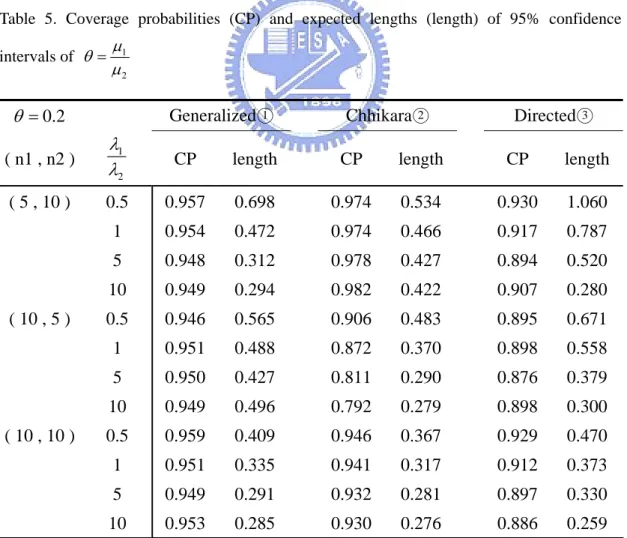
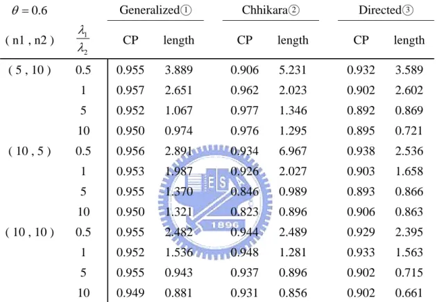
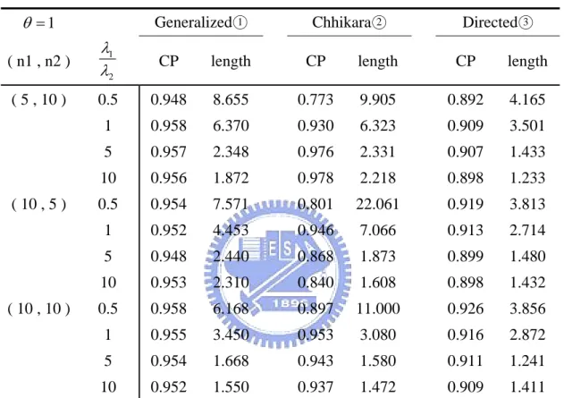
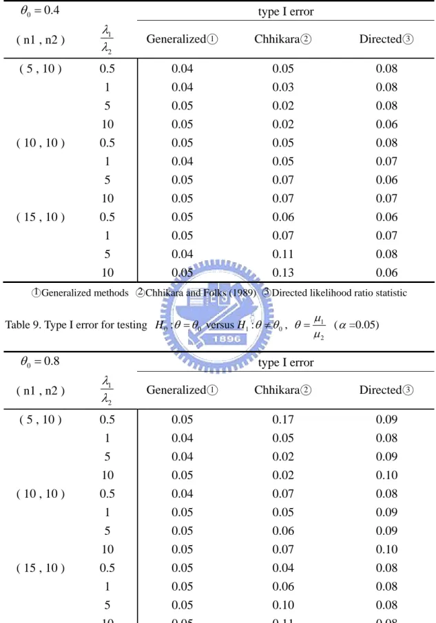
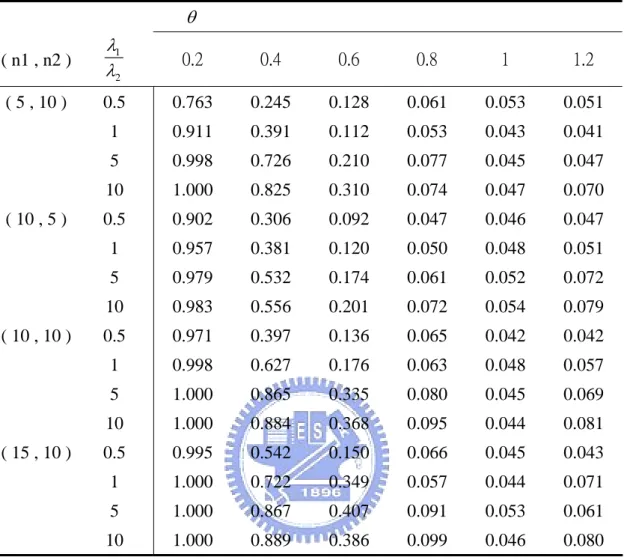
respect to their confidence intervals and confidence lengths. Several simulation studies are also presented to compare the performances of three methods, (1) Chhikara and Folks (2) Tian and Wilding (3) the generalized approaches, in terms of their coverage probabilities, expected lengths and the Type I error.

5.1

Numerical examples

Example 1.

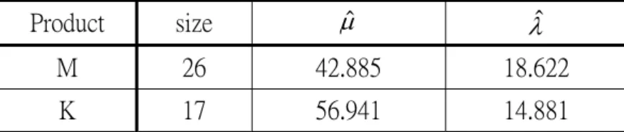
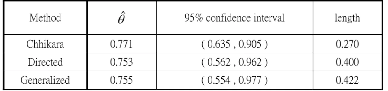
Gacula and Kubala (1975) reported certain sensory failure data for two refrigerated food products, M and K as these were called, and studied their shelf life which fit the IG distribution well. The summary data are given in Table 1 and the 95% confidence intervals for three methods are presented in Table 2.

Table 1. Summary data

Product size μˆ _λ ˆ

M 26 42.885 18.622

Table 2. 95% confidence intervals and lengths for 1 2 μ θ μ =

Method

_θ

ˆ

95% confidence interval length Chhikara 0.771 ( 0.635 , 0.905 ) 0.270

Directed 0.753 ( 0.562 , 0.962 ) 0.400 Generalized 0.755 ( 0.554 , 0.977 ) 0.422

Example 2.

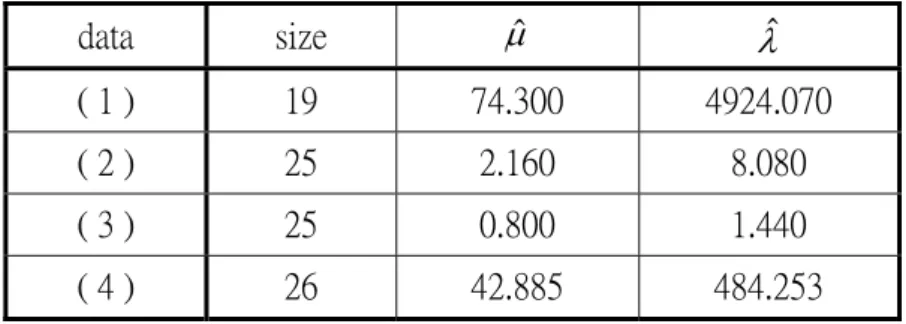
Four sets of IG data presented in Folks and Chhikara (1978) who judged that the data are very well described by the Inverse Gaussian distribution. The first set, data (1), gives fracture toughnesses of MIG welds. The second set, data (2), gives data of precipitation (inches) from Jug Bridge, Maryland. The third set, data (3), gives runoff amounts at Jug Bridge, Maryland. Additionally, Gacula and Kubala (1975) gave data (4) on shelf-life of a food product. The summary data for four sets of IG data are shown in Table 3. For investigating the ratio of means of two independent populations when the scale parameters are more different than those in Example 1, we will compare the means of these four data sets mutually and show the results in Table 4.

Table 3. The summary data for four data sets data size μˆ _λ ˆ ( 1 ) 19 74.300 4924.070 ( 2 ) 25 2.160 8.080 ( 3 ) 25 0.800 1.440 ( 4 ) 26 42.885 484.253

Table 4. 95% confidence intervals and lengths for 1

2

μ θ

μ

=

(2)/(1)

_θ

ˆ

95% confidence interval length Chhikara 0.0303 ( 0.020 , 0.040 ) 0.020 Directed 0.0290 ( 0.024 , 0.036 ) 0.012 Generalized 0.0294 ( 0.024 , 0.037 ) 0.014

(3)/(1)

_θ

ˆ

95% confidence interval length Chhikara 0.0118 ( 0.006 , 0.017 ) 0.011 Directed 0.0108 ( 0.008 , 0.016 ) 0.008 Generalized 0.0111 ( 0.008 , 0.016 ) 0.008

(4)/(1)

_θ

ˆ

95% confidence interval length Chhikara 0.5857 ( 0.469 , 0.702 ) 0.233 Directed 0.5771 ( 0.509 , 0.661 ) 0.152 Generalized 0.5796 ( 0.505 , 0.667 ) 0.162

(3)/(2)

_θ

ˆ

95% confidence interval length Chhikara 0.4046 ( 0.154 , 0.655 ) 0.501 Directed 0.3726 ( 0.262 , 0.558 ) 0.296 Generalized 0.3812 ( 0.258 , 0.564 ) 0.306

(2)/(4)

_θ

ˆ

95% confidence interval length Chhikara 0.0521 ( 0.034 , 0.070 ) 0.036 Directed 0.0503 ( 0.040 , 0.066 ) 0.026 Generalized 0.0509 ( 0.040 , 0.065 ) 0.025

(3)/(4)

_θ

ˆ

95% confidence interval length Chhikara 0.0201 ( 0.011 , 0.029 ) 0.018 Directed 0.0187 ( 0.014 , 0.028 ) 0.014 Generalized 0.0193 ( 0.014 , 0.028 ) 0.014

From Example 1 and Example 2, the results show that the confidence lengths

obtained by the generalized methods are the smallest or close to the smallest confidence lengths no matter what the scale parameters perform when two IG populations are non-homogeneous. Some simulation studies are also worth to be inspected, and we will make discussion in next subsection.